
Select actionable positive or negative sequential patterns
Abstract
Negative sequential patterns (NSP) refer to sequences with non-occurring and occurring items, and can play an irreplaceable role in understanding and addressing many business applications. However, some problems occur after mining NSP, the most urgent one of which is how to select the actionable positive or negative sequential patterns. This is due to the following factors: 1) positive sequential patterns (PSP) mined before considering NSP may mislead decisions; and 2) it is much more difficult to select actionable patterns after mining NSP, as the number of NSPs is much greater than PSPs. In this paper, an improved method of pruning uninteresting itemsets to fit for a selecting actionable sequential pattern (ASP) is proposed. Then, a novel and efficient method, called SAP, is proposed to select the actionable positive and negative sequential patterns. Experimental results indicate that SAP is very efficient in the selection of ASP. To the best of our knowledge, SAP is the best method for the selection of actionable positive and negative sequential patterns.
1Introduction
Negative sequential patterns (NSP) refer to sequences with non-occurring and occurring items, while sequential patterns that contain only occurring items are called positive sequential patterns (PSP) [19, 24, 26]. For instance, assume that p 1 =< abcX > is a PSP; p 2 =< abcY > is an NSP, where a, b and c represent medical service codes that a patient has received in a healthcare setting, and X and Y each stand for a disease status. p 1 indicates that a patient who usually receives medical services a, b and then c is likely to have disease status X, whereas p 2 indicates that patients receiving treatment of a and b but not c have a high probability of disease status Y. It is increasingly recognized that such NSPs can play an irreplaceable role in understanding and addressing many business applications, such as associations between treatment services and illnesses. However, some urgent problems occur after mining NSP. These urgent problems include: 1) difficult in selecting actionable positive or negative sequential patterns; 2) the need to improve efficiency of the NSP mining algorithm; 3) how to decrease the number of negative sequential candidates (NSC). Among these problems, the selection problem is the most urgent.
One reason for this is that the PSPs being mined before considering NSP may mislead decisions. For example, a PSP < abc > was mined and used to make decisions before considering NSP. However, based on < abc >, NSPs such as < abc >, < abc >, < abc > and < abc > may be obtained. Obviously, not all of these patterns are actionable. If < abc > is not actionable now, the previous decisions that are made based on it would be incorrect.
Another reason is that it is much more difficult to select actionable patterns after mining NSP, because the number of NSPs is much greater than PSPs. To a k-size of PSP p, the number of potential negative sequential patterns based on p, |NSP
p
|, according to a NSP mining algorithm e-NSP [24], is
Although there have been some reports of actionable knowledge discovery [8, 9, 10, 16] and selecting actionable patterns/rules or interestingness measures in association rule mining [1, 2, 4, 15, 17], none of the previous research considers how to select actionable positive and negative sequential patterns. Very few papers study NSP mining [12, 19, 20, 21, 24, 26, 27], and most primarily focus on how to design a mining algorithm and how to improve the algorithm’s efficiency. Therefore, this paper investigates association rule mining. In this area, some methods have been proposed to prune uninteresting itemsets, to select actionable patterns, to mine positive and negative association rules, and so on [2, 4, 15, 17]. Among these methods, the one proposed by X.D. Wu, et al. is one of the most suitable methods, referred to as Wu’s method for convenience [23]. Wu’s method can prune the itemsets that are not of interest before mining positive and negative association rules. However, due to the differences between the association rule and sequential pattern, this method cannot be directly used to solve the selection problem and must be improved before use.
No studies shave yet applied Wu’s method to positive or negative sequential patterns, and Wu’s method can only deal with itemsets, not actionable sequential patterns. Therefore, in this paper, we first improve Wu’s method to fit a selecting actionable sequential pattern (ASP), then propose a novel and efficient method, called SAP, to select actionable positive and negative sequential patterns based on the improved method. Experimental results indicate that SAP is very efficient in the selection of ASP. To the best of our knowledge, this is the best method to select actionable positive and negative sequential patterns.
The remainder of the paper is organized as follows. Section 2 discusses the related work. In Section 3 reviews an e-NSP algorithm and Wu’s method, and then proposes the improved method and SAP method. Section 4 presents the experiment results, and conclusions and future work are presented in Section 5.
2Related work
Some literature has proposed a few measures to mine interesting association rules, such as correlation coefficients, chi-squared tests, interestingness, Laplace, the Gini-index, Piatetsky-Shapiro method, conviction and so on [2, 4, 15, 17]. M.L. Antonie, O.R. Zaiane, X.J. Dong, Z.D. Niu, X.L. Shi, X.D. Zhang and D.H. Zhu used correlation coefficient to mine positive and negative association rules [11, 25]. B. Liu, W. Hsu and Y.M. Ma used chi-squared test to prune non-actionable rules or rules at lower significance levels [3].
Some literature has discussed the selection of actionable knowledge or actionable patterns. L.B. Cao, C.Q. Zhang, et al. developed a new data mining framework, referred to as Domain-Driven In-Depth Pattern Discovery (DDID-PD) [8]. L.B. Cao, Y.C. Zhao, et al. formally defined the actionable knowledge discovery (AKD) concepts, processes, the action ability of patterns, and operable deliverables. With such components, four types of AKD frameworks are proposed to handle various business problems and applications [9]. L.B. Cao discussed a paradigm shift in knowledge discovery from data to actionable knowledge discovery and delivery. In post-analysis [10], a key component is to extract actions from learned rules [23]. A typical method applied to learning action rules is to split attributes into “hard/soft” [23] to extract actions that may improve the loyalty or profitability of customers. G. Adomavicius and A. Tuzhilin proposed a method of discovery of actionable patterns, which first builds an action tree for the specific application, and then assigns actionable patterns to the corresponding nodes of the tree by data mining queries [5]. K. Kavitha and E. Ramaraj proposed an efficient transaction reduction algorithm, TR-BC, to mine the frequent patterns based on bitmap and class labels [6]. K. Wang, Y. Jiang and A. Tuzhilin introduced the notion of “action” as a domain-independent method to model the domain knowledge. This presents several pruning strategies to reduce the search space and algorithms for mining all actionable patterns, as well as mining the top k actionable patterns [7]. P. Kanikar and D.K. Shah extracted actionable association rules from multiple datasets [14].
Next, the literature on mining NSP is discussed.
S.C. Hsueh, M.Y. Lin and C.L. Chen proposed a PNSP approach for mining positive and negative sequential patterns in the form of < (abc)¬ (de) (ijk) > [19]. Z.G. Zheng, Y.C. Zhao, Z. Zuo and L.B. Cao proposed an NegGSP approach to mine NSP. The general idea of NegGSP is to mine PSPs by GSP first, then to generate and prune NSCs. After that, it counts the support of NSCs by re-scanning databases to identify negative patterns [26]. N.P. Lin, H.J. Chen and W.H. Hao only mined NSPs whose final element is negative and other elements are positive [12]. W.M. Ouyang and Q.H. Huang only identified NSP in the form of (¬ A, B) , (A, ¬ B) and (A, ¬ B) [21], which is similar to mine negative association rules [13, 23].
This requires A∩ B = ∅, which is a usual constraint to association rule mining but is represents a very strict constraint to sequential pattern mining. V.K. Khare and V. Rastogi mined NSP in the same form as W.M. Ouyang and Q.H. Huang in incremental transaction databases [12, 21]. Z.G. Zheng, Y.C. Zhao, Z. Zuo and L. Cao proposed an approach based on genetic algorithms to mine NSPs. The approach borrows the idea of gene evolution, to obtain candidates by crossover and mutation, and proposed a dynamic fitness function to generate as many candidates as possible and to avoid population stagnation [27].
X.J. Dong, Z.G. Zheng, L.B. Cao, Y.C. Zhao, et al. proposed an efficient e-NSP algorithm to mine NSP. In this paper, e_NSP is used to mine PSPs and NSPs. The details of e_NSP will be introduced in Section 3 [24].
3SAP method
3.1Basic concept
Let I = {i 1, i 2, …, i n } be a set of items; an itemset is a subset of I and a sequence is an ordered list of itemsets. A sequence s is denoted by <s 1, s 2… s 1 >, where s j ⊆ I for 1 ≤ j ≤ 1. s j is also designated as an element of the sequence, and denoted as (x 1, x 2 … x m ), where x k is an item, x k ∈ I for 1 ≤ k ≤ m. For brevity, the brackets are omitted if an element has only one item; for example, element (x) is written as x. The order number j of element s j is called order_id of s j , denoted as id (s j ), i.e., id (s j ) = j. An item can occur once, at most, in an element of a sequence, but can occur multiple times in different elements of a sequence. The length of sequence s, denoted as length(s), is the total number of items in all the elements in s; sequence s is a k-length sequence if length(s) = k. The size of sequence s, denoted as size(s), is the total number of elements in s; sequence s is a k-size sequence if size(s) = k. For example, s 1 =< abc > is a 3-length, 3-size sequence; s 2 =< (ab) c > and s 3 =< a (bc) > are both 3-length, 2-size sequences.
Sequence α =< α 1, α 2 … α n > is a subsequence of sequence β =< β 1, β 2 … β m > and β is a super sequence of α, denoted as α ⊆ β, if there exist integers 1 ≤ j 1 < j 2 < … < j n ≤ m such that β contains α. For example, <a (cd)> is a subsequence of<ab (cde)>, <ab (cde)> is a super subsequence of <a (cd)> also denoted as <ab (cde)> contains<a (cd)>.
A sequence database D is a set of tuples <sid, ds>, where sid is a sequence _ id, and ds is a data sequence. The number of tuples in D is denoted as |D|. The set of tuples containing sequence α is denoted as {< α >}. The support of α, denoted as s (α), is the ratio of the number of {< α >} to the total number of tuples in D, i.e., s (α) = | {< α >} |/|D| = | {< sid, ds > | < sid, ds > D (α ds)} |/ |D|. The ms is a minimum support threshold given by users or experts. Sequence α is called a (positive) sequential pattern, or α is frequent, if s (α) ≥ ms; α is infrequent, if s (α) < ms. The task of positive sequential pattern mining is to discover the set of all positive sequential patterns.
The concepts of length and size for positive sequences are also suitable for negative sequences. The neg-size of sequence ns, denoted as neg-size(ns), is the total number of negative elements in ns; ns is a k-neg-size negative sequence if neg-size(ns) = k. For example, ns =< ¬ a (ab) ca ¬ c > is a 5-size and 2-neg-size negative sequence because size(ns) = 5 and neg-size(ns) = 2.
3.2Review of e_NSP
3.2.1Three constraints in e_NSP
An e_NSP adds three constraints to negative sequences in order to decrease the number of NSCs and discover only meaningful NSPs.
Constraint 1 is the element negative constraint. That is, the minimum negative unit in am NSC is an element; not only one part of the items in the element (if the element includes more than one item) is negative. For example, <a¬ (ab) ca ¬ c > satisfies this constraint, but not the <a (¬ ab) ca ¬ c > because only a is negative in element (¬ ab).
Constraint 2 is formation constraint. There are no contiguous negative elements in an NSC because right order of two contiguous negative elements cannot be determined if there are no positive elements between them. For example, <a¬ (ab) ca ¬ c > satisfies constraint 2, but not the <a¬ (ab) c ¬ a ¬ c >.
Constraint 3 is frequency constraint. The e_NSP only mined the NSP whose positive partner is a PSP. The positive partner of a negative sequence changes all negative elements in ns to their corresponding elements, denoted as p (ns). For example, p (< a ¬ (ab) ca ¬ c >) = < a (ab) cac >
3.2.2The main steps of e_NSP
There are four steps in e_NSP.
– The first step is to mine all PSPs according to the classical PSP mining algorithms. To each PSP p, save its support and all sid of the data sequence that contain the p to a set {p}.
– Based on these PSPs, generate all NSCs according to the following method.
– For a k-size PSP, its NSCs are generated by changing any m non-contiguous element to its negative element, m = 1, 2, …, [k/2], where [k/2] is a minimum integer that is no less than k/2. For example, the NSCs based on <abcde> include: m = 1, < abcde > , < abcde > , < abcde > , < abcde > , < abcde > ; m = 2, < abcde > , < abcde > , < abcde > , < abcde > , < abcde > , < abcde > ; m = 3, < abcde > .
– Convert the negative containment to a positive containment.
– For example, if a data sequence ds contains negative sequence <¬ ab ¬ cd ¬ e >, then ds must contain (positive) sequence <bd> and must not contain (positive) sequence <abd>, <bcd> and <bde>.
– Calculate the support of each NSC and determine whether it is a NSP by comparing its support with the minimum threshold ms.
For example, s (< abcde >) = s (< bd >) - | {< abd >} ∪ {< bcd >} ∪ {< ! bde >} |/|D|, where {< abd >},{< bcd >} and {< bde >} are the sid set that contain <abd> , < bcd > and <bde> respectively, and | {< abd >} ∪ {< bcd >} ∪ {< bde >} | is the sid number of the union set.
3.3The original Wu’s method
Wu’s method defines an interestingness function interest (X, Y) = |s (X ∪ Y) | - s (X) s (Y) | and a threshold mi (minimum interestingness) [23]. If interest (X, Y) mi, the rule of X and Y is of potential interest, and X and Y are referred to as a potentially interesting itemset. The details are as follows.
I is a frequent itemset of potential interest if
fipi(I) = s(I) ≥ ms ∧
(1)
(2)
(3)
where f() is a constraint function concerning the support, confidence, and interestingness of X and Y; and ms, mc, mi are the minimum support, minimum confidence, and minimum interestingness provided by users or experts.
Using this method, Wu’s method can establish an effective pruning strategy for efficiently identifying all frequent itemsets. However, due to the differences between itemsets and sequential patterns, this method can’t be directly used to solve the selection problem and must be improved before use.
3.4The improved Wu’s method
The improvements cover three aspects; the third improvement is the key improvement.
– Remove the confidence measure from Equations 1–3.
The confidence measure c() and mc are used to discover association rules. If only itemsets/ patterns are discovered, this measure can be removed, as in Wu’s method.
– Replace the interestingness function with correlation coefficient function.
X.J. Dong explains that interest (X, Y) is not enough to prune uninteresting itemsets because it is greatly influenced by the value of s (X ∪ Y), s (X) and s (Y). For example, interest of (X, Y) is no more than 0.1 if s (X ∪ Y), s (X) and s (Y) are less than 0.1; interest of (X, Y) is no more than 0.01 if s (X ∪ Y), s (X) and s (Y) are less than 0.01. s (X ∪ Y), s (X) and s (Y) are variable with different datasets or different itemsets, so that it is very difficult for users to designate mi a suitable value [22]. X.J. Dong analyzed this shortcoming and proposed a good substitute: the correlation coefficient [22]. Correlation coefficients can also measure the relationships between X and Y, and change with the degree of linear dependency between X and Y. More details can be found in [22]. Here, we simply adopt this result and use a correlation coefficient instead of interest (X, Y).
The correlation coefficient between X and Y, ρ (X, Y), can be calculated as follows:
(4)
ρ (X, Y) has the following three possible cases:
* If ρ (X, Y) <0, then X and Y are positively correlated. The more X events that occur, the more Y events occur.
* If ρ (X, Y) =0, then X and Y are independent (for binary variables). The occurrence of event X has nothing to do with the occurrence of event Y.
* If ρ (X, Y) >0, then X and Y are negatively correlated. The more X events occur, fewer Y events occur
The range of ρ (X, Y) is between –1 and +1, and the positive correlation is between the absolute value of ρ (X, Y), and represents the correlation strength of A and B. Therefore, we can set a threshold ρmin to prune patterns with small correlation strength.
Correspondingly, we replace interest (X, Y) with ρ (X, Y) and remove the confidence measure. Then, Equations (2) and (3) are simplified to Equations (5) and (6).
(5)
(6)
– Adapt these equations to fit sequential patterns.
So far, the above discussions are based on mining interesting itemsets, not sequences. The differences between them are that, in a sequence, the itemsets are in an order, and an item can occur at multiple times in different elements of a sequence. Therefore, the conditions ∃X, Y : X ∪ Y = I and X ∩ Y = Φ in Equations 4-5 must be changed; how they are changed is the key technique for selecting ASP. Our methods test whether any 2-size sequence constructed by two contiguous elements in a pattern is actionable. That is, if a k-size (k > 1) PSP or NPS P =< ele2 … ek > is actionable, then we require that <ele2>, <e2e3>, …, <ek - 1ek> be actionable too. Formally, we have the following definitions.
Definition 1. Actionable sequential pattern.
A k-size (k > 1) PSP or NSP P =< e1 e2 … ek > is an actionable sequential pattern if ∀i ∈ {2 … k},
(7)
(8)
(9)
According to Definition 1, we can obtain a corollary as follows.
Corollary 1. A k-size (k > 1) PSP or NSP P =< e 1 e 2 … e k > is not an ASP if ∃i ∈ {2 … k},<e i-1 e i > is not an ASP.
Proof. From Definition 1, we can see that if P =< e 1 e 2 … e k > is an ASP, then ∀i ∈ {2 … k}, <e i-1 e i > must be an ASP. Otherwise, P =< e 1 e 2 … e k > will not be an ASP. This satisfies corollary 1, so corollary 1 is correct.
Definition 1 and correlary 1 are used to implement the proposed SAP method
3.5SAP method
The primary steps of SAP method are as follows.
Step 1: all PSP and NSP are mined by e-NSP.
Step 2: each 2-size pattern such s< e 1 e 2 > are tested by Definition 1. If <e 1 e 2> is not an ASP, then<e 1 e 2> and all the patterns containing <e 1 e 2> are removed.
Step 3: longer sized patterns are tested in a similar way as step 2, until all patterns are tested.
Algorithm SAP.
Input: D: a sequential database; ms: minimum support; ρmin: a threshold defined by user;
Output: ASP: set of actionable sequential patterns;
- let ASP =Φ:
- use e-NSP to mine all PSPs and NSPs and store them in the set {PNSP};
- for k = 2 to maximum length of PSP in {PNSP} do {
- for each k-size pattern P< e 1 e 2 … e k > in {PNSP} do {
- test P with definition 1;
- if P is an actionable sequential pattern then
- ASP = ASP∪{P};
- else
- remove P and all the patterns contain P from PNSP;
- end if
- }
- k++;
- }
- return ASP;
An example is illustrated below.
The sample database is shown in Table 1, given ms = 0.4, and ρ min = 0.3.
Step 1: Use e-NSP algorithm to mine all PSP and NSP. We obtain:
PSP = {<a>, <b>, <c>, <d>, <e>, <f>, <aa>, < (ab)>, <ab>, <ba>, <ac>, <ca>, <ad>, <ea>, <af>, < (bc)>, <bc>, <cb>, <bd>, <db>, <eb>, <bf>, <fb>, <cc>, <dc>, <ec>, <fc>, <ef>, < (ab)c>, < (ab)d>, < (ab)f>, <aba>, <eab>, <a(bc)>, <abc>, <aca>, <eac>, <acb>, <acc>, < (bc)a>, <adc>, <ebc>, <fbc>, <dcb>, <ecb>, <fcb>, <bdc>, <efb>, <efc>, < (ab)dc>, <a(bc)a>, <eacb>, <efcb> }.
NSP = {< ¬ f > , < ¬ aa > , < a ¬ a > , < ¬ (ab) > , < ¬ ba > , < b ¬ a > , < ¬ ca > , < c ¬ a > , < ¬ ad > , < a ¬ d > , < ¬ ea > , < e ¬ a > , < a ¬ f > , < ¬ (bc) > , < ¬ bd > , < b ¬ d > , < ¬ db > , < d ¬ b > , < ¬ eb > , < e ¬ b > , < b ¬ f > , < ¬ fb > , < ¬ ec > , < e ¬ c > , < ¬ fc > , < e ¬ f > , < ¬ (ab) c > , < ¬ (ab) d > , < ab ¬ a > , < ¬ eab > , < a ¬ (bc) > , < a ¬ bc > , < ab ¬ c > , < ac ¬ a > , < ¬ eac > , < ¬ (bc) a > , < a ¬ dc >} .
Step 2: test all actionable sequential patterns according to Definition 1 and corollary 1. Some examples are listed below.
For <ab>, s(<ab>) = 0.8, s(<a>) = 0.8, s(<b>) = 0.8
Sequence <ab>meets asp(a, b) = s(<ab>) ≥ 0.4 ∧ (f (a, b, ms, ρmin) = 1), so it is an asp.
For <cb>, s(<cb>) = 0.6, s(<c>) = 0.8, s(<b>) = 0.8
Therefore <cb>is not an asp.
For < ¬ eab > , s (< ¬ ea >) = 0.4, s (< ¬ e >) = 0.2, s (< a >) = 0.8
We require test sequence <¬ ea > and sequence <ab>; if each of these sequences is an ASP, <¬ eab > is also an ASP.
Sequence <¬ ea > meets asp(¬ e, a) = s (< ¬ ea >) ≥ 0.4 ∧ (f (¬ e, a, ms, ρmin) = 1) ; test sequence <ab>is an ASP, therefore <¬ eab > is an ASP.
All ASPs are obtained according to the above procedure.
ASP = {< ab > , < ac > , < (ab) c > , < (ab) d > , < (ab) f > , < a (bc) > , < (bc) a > , < a (bc) a > , < ¬ aa > , < a ¬ a > , < ¬ ba > , < b ¬ a > , < ¬ ca > , < c ¬ a > , < ¬ ad > , < a ¬ d > , < ¬ ea > , < e ¬ a > , < a ¬ f > , < ¬ bd > , < b ¬ d > , < ¬ db > , < d ¬ b > , < ¬ eb > , < e ¬ b > , < b ¬ f > , < ¬ fb > , < ¬ ec > , < e ¬ c > , < ¬ fc > , < e ¬ f > , < ab ¬ a > , < ¬ eab > , < ac ¬ a > , < ¬ eac >} .
4Experimental results
Experiments were performed on a Pentium 4 Celeron 2.1 G PC with 2 G main memory, running on Microsoft Windows7. All programs were written in MyEclipse 10.
4.1Datasets
To describe and observe the impact of data characteristics on algorithm performance, the following data factors are used: C, T, S, I, DB and N, which are defined to describe characteristics of sequence data [18].
C: Average number of elements per sequence;
T: Average number of items per element;
S: Average size of maximal potentially large sequences;
I: Average size of items per element in maximal potentially large sequences;
DB: Number of sequences (=size of Database); and
N: Number of items.
Four source datasets are also used in these experiments [24]. They include both real data and synthetic datasets generated by an IBM data generator [18].
Dataset 1 (DS1), C8_T4_S6_I6_DB100k_N0.1k.
Dataset 2 (DS2), C10_T8_S20_I10_DB10k_N0.2k.
Dataset 3 (DS3) is obtained from UCI Datasets. There are 989,818 records; average number of elements in a sequence is 4; and each element only has one item.
Dataset 4 (DS4) is real-application data from the financial service industry. It contains 5,269 customers/sequences; the average number of elements in a sequence is 21; the minimum number of elements in a sequence is 1; and the maximum number is 144.
4.2Experimental results
In the experiments, different ms and ρ min values were set to reflect differences in the four datasets. The results of the experiment are as follows:
4.3Experimental analysis
Figures 1–4 demonstrate that with the increment of ρ min, the number of actionable sequential patterns decreases based on the same minimum support. As shown in Fig. 1, we set ms = 0.14. The experimental data are synthetic data with an increment of ρmin, the number of actionable sequential patterns downward trend is flat, and the running time downward trend is flat. With the same synthetic data, the experimental results in Figs. 1 and 5 are identical to results shown in Figs. 2 and 6. In Fig. 3, ms = 0.01, which is much lower than the value in the synthetic data, is closer to the real-world number. Therefore, the experimental result is close to the real-world result, which proves that the proposed method can be used in businesses applications. As shown in Figs. 3 and 4, with the increase of ρmin, the downward trend in the number of actionable sequential patterns is not a steady decline, but demonstrates some variation. As shown in Figs. 7 and 8, the running time trend is the same as in Figs. 5 and 6, which proves that our proposed method has a stable running time.
Because our method was conducted after the improvement of Wu’s method and Wu’s method cannot be used for processing sequence, our proposed method cannot be directly compared to Wu’s method. However, our data are all sequence data. Further, There is no method can be used to compare.
These experimental results indicate that our proposed method demonstrates a proven stable running result and running time. The problem of selecting the actionable positive and negative sequential patterns is solved through our method. By setting the parameter close to the real-world parameter, SAP determination can efficiently deal with both synthetic and real-world databases.
5Conclusions and future work
It is increasingly recognized that NSP can play an irreplaceable role in understanding and addressing many business applications. However, some urgent problems occur after mining NSP. These urgent problems include: 1) a selection problem; 2) efficiency problem; 3) candidate problem; and other concerns. Among these problems, the selection problem is the most urgent because the PSP being mined before considering NSP may mislead decisions, and it is much more difficult to select actionable patterns after mining NSP due to the huge number of NSPs. This paper proposes an improvement to Wu’s pruning method to fit for selecting ASP. A novel method is proposed to efficiently use SAP to select ASP. Experimental results indicate that SAP is very efficient.
Future work will find solutions to other urgent problems.
Acknowledgments
This work was supported partly by National Natural Science Foundation of China (71271125, 61173061 and 71201120), Natural Science Foundation of Shandong Province, China (ZR2011FM028) and Scientific Research Development Plan Project of Shandong Provincial Education Department (J12LN10).
References
1 | Tzacheva A, Ras Z (2005) Action rules mining International Journal of Intelligent Systems 20: 719 736 |
2 | Liu B, Hsu W, Chen S, Ma YM (2000) Analyzing subjective interestingness of association rules IEEE Intelligent Systems 15: 5 47 55 |
3 | Liu B, Hsu W, Ma YM (2001) Identifying non-actionable association rules Proceedings of the ACM SIGKDD International Conference on Knowledge Discovery and Data Mining 329 334 San Francisco, CA, USA |
4 | Omiecinski ER (2003) Alternative interest measures for mining associations IEEE Trans Knowledge and Data Eng 15: 1 57 69 |
5 | Adomavicius G, Tuzhilin A (1997) Discovery of actionable patterns in databases: The action hierarchy approach 111 114 KDD, California, USA |
6 | Kavitha K, Ramaraj E (2013) Efficient transaction reduction in actionable pattern mining for high voluminous datasets based on bitmap and class labels International Journal on Computer Science and Engineering 5: 7 664 671 |
7 | Wang K, Jiang Y, Tuzhilin A (2006) Mining actionable patterns by role models Proceedings of the International Conference on Data Engineering 2006: 16 16 |
8 | Cao LB, Zhang CQ (2007) Domain-driven actionable knowledge discovery IEEE Intelligent Systems 22: 4 78 88 |
9 | Cao LB, Zhao YC (2010) Flexible frameworks for actionable knowledge discovery IEEE Transactions on Knowledge and Data Engineering 22: 9 1299 1312 |
10 | Cao LB (2012) Actionable knowledge discovery and delivery WIREs Data Mining and Knowledge Discovery 2: 2 149 163 |
11 | Antonie ML, Zaiane OR (2004) Mining positive and negative association rules: An approach for confined rules Knowledge Discovery in Databases: PKDD 3202: 27 38 |
12 | Lin NP, Chen HJ, Hao WH (2007) Minin negative sequential patterns 654 658 WSEAS, Hangzhou China |
13 | Lin NP, Chen HJ, Hao WH (2007) Minin negative fuzzy sequential patterns Proceedings of the 7th WSEAS International Conference on Simulation, Modeling and Optimization 52 57 Beijing, China |
14 | Kanikar P, Shah DK (2012) Extracting actionable association rules from multiple datasets International Journal of Engineering Research and Applications 2: 3 1295 1300 |
15 | Tan PN, Kumar V, Srivastava J (2002) Selecting the right interestingness measure for association patterns Proceedings of the ACM SIGKDD International Conference on Knowledge Discovery and Data Mining 32 41 Edmonton, Alta, Canada |
16 | Yang Q, Yin J, Ling C, Pan R (2007) Extracting actionable knowledge from decision trees IEEE Trans Knowledge and Data Eng 19: 1 43 55 |
17 | Hilderman RJ, Hamilton HJ (2000) Applying objective interestingness measures in data mining systems Proceedings of the 4th European Symposium on Principles of Data Mining and Knowledge Discovery (PKDD’00) 432 439 France |
18 | Agrawal R, Srikant R (1995) Minin sequential patterns 3 14 ICDE Taipei |
19 | Hsueh SC, Lin MY, Chen CL (2008) Mining negative sequential patterns for e-commerce recommendations Asia-Pacific Services Computing Conference 1213 1218 Yilan, Taiwan |
20 | Khare VK, Rastogi V (2013) Mining positive and negative sequential pattern in incremental transaction databases International Journal of Computer Applications 71: 1 18 22 |
21 | Ouyang WM, Huang QH (2007) Mining negative sequential patterns in transaction databases Machine Learning and Cybernetics 2: 830 834 |
22 | Dong XJ (2011) Mining interesting infrequent and frequent itemsets based on minimum correlation strength Lecture Notes in Computer Science 7002: 437 443 |
23 | Wu XD, Zhang CQ, Zhang SC (2004) Efficient mining of both positive and negative association rules ACM Trans Inf Syst 22: 3 381 405 |
24 | Dong XJ, Zheng ZG, Cao LB, Zhao YC (2011) E-NSP: Efficient negative sequential pattern mining based on identified positive patterns without database rescanning International Conference on Information and Knowledge Management 825 830 Glasgow, UK |
25 | Dong XJ, Niu ZD, Shi XL, Zhang XD, Zhu DH (2007) Mining both positive and negative association rules from frequent and infrequent itemsets Advanced Data Mining and Applications 4632: 122 133 |
26 | Zheng ZG, Zhao YC, Zuo Z, Cao LB (2009) Negative-gsp: An efficient method for mining negative sequential patterns Data Mining and Analytics 101: 63 67 |
27 | Zheng ZG, Zhao YC, Zuo Z, Cao L (2010) An efficient ga-based algorithm for mining negative sequential patterns PAKDD 6118: 262 273 |
Figures and Tables
Fig.1
The count of actionable sequential patterns.
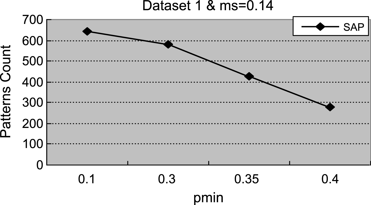
Fig.2
The count of actionable sequential patterns.
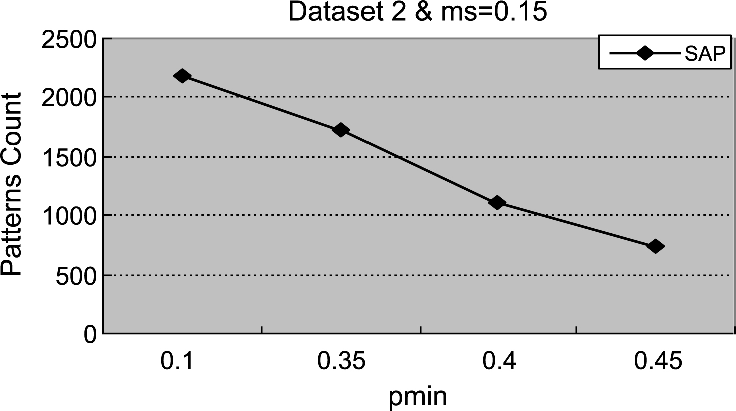
Fig.3
The count of actionable sequential patterns.
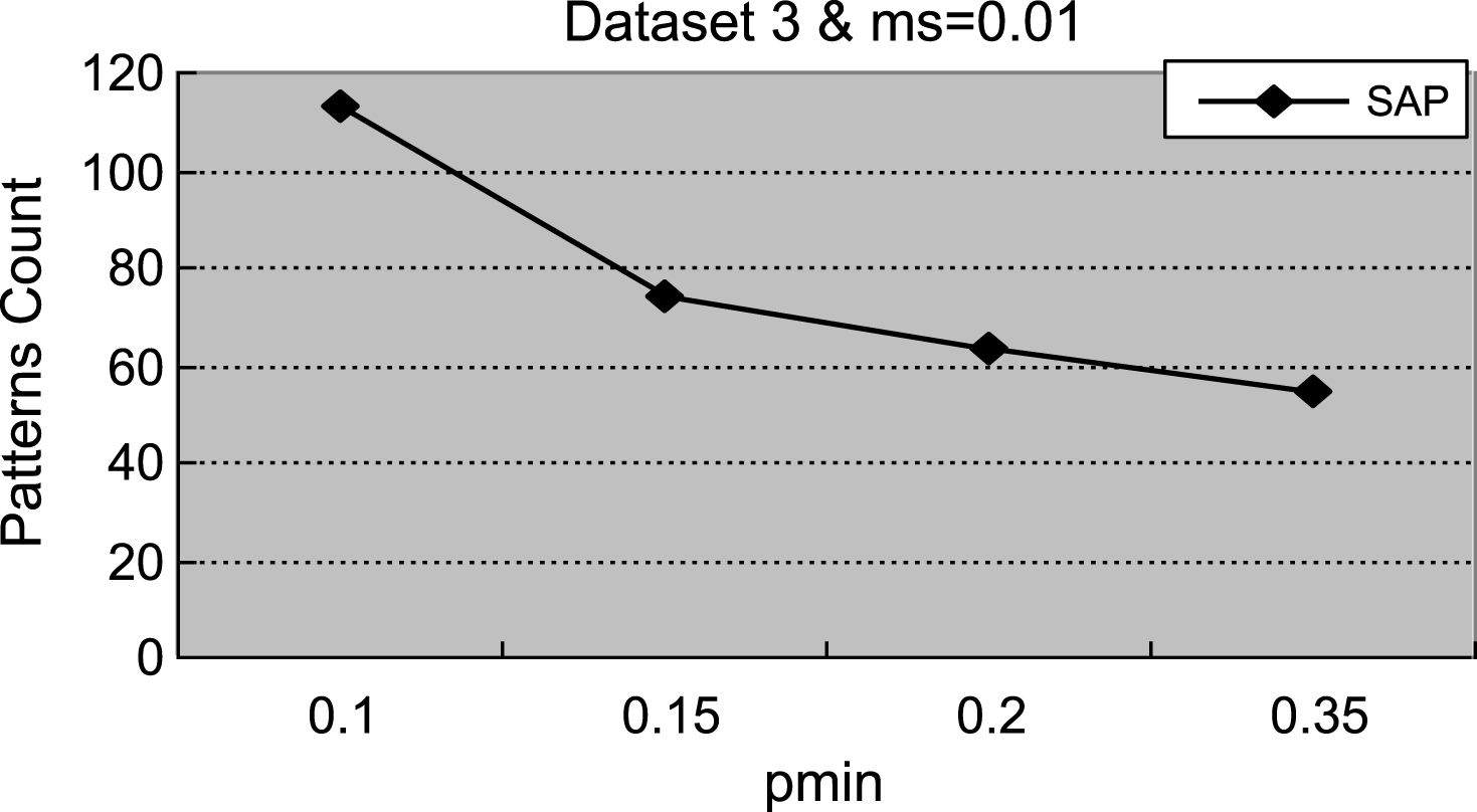
Fig.4
The count of actionable sequential patterns.
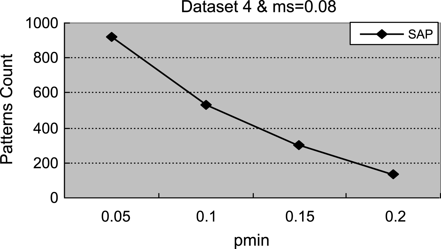
Fig.5
Running time (s).
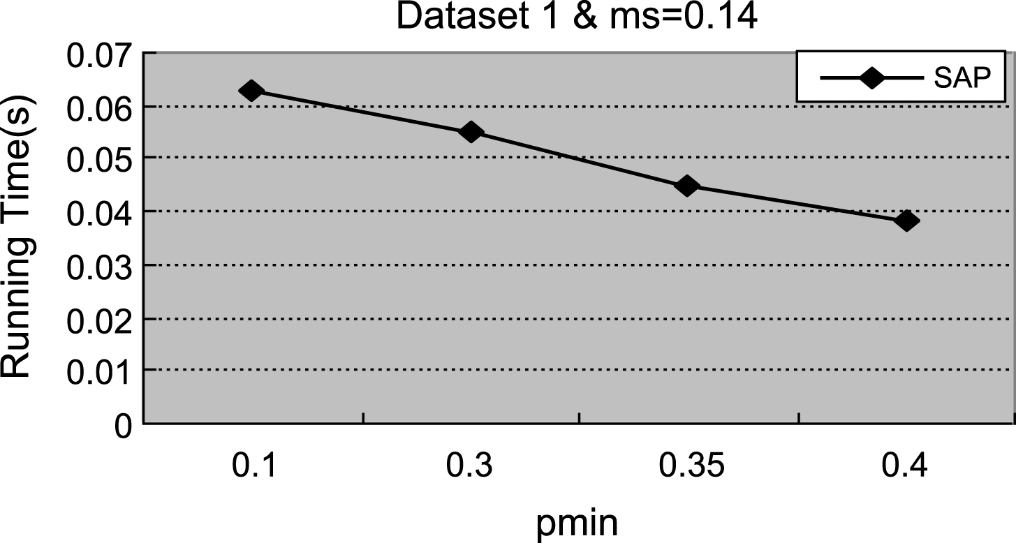
Fig.6
Running time(s).
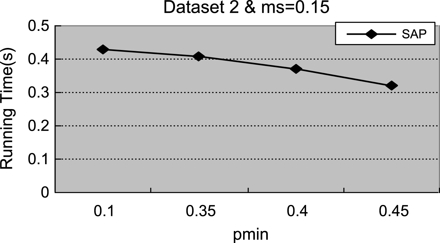
Fig.7
Running time (s).
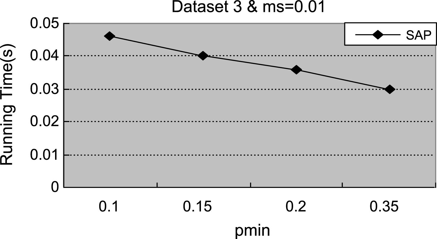
Fig.8
Running time (s).
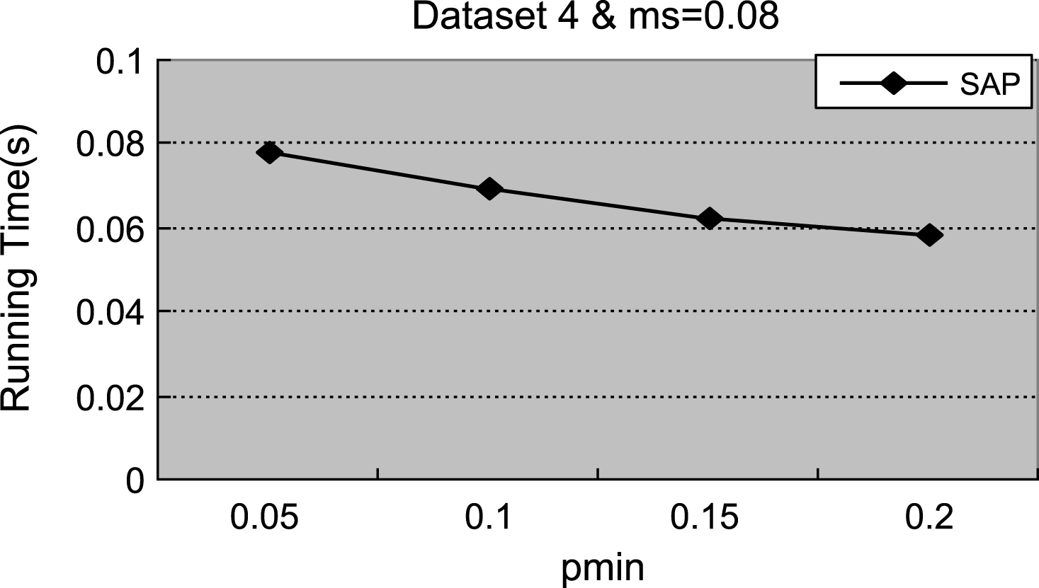
Table 1
Sample database
| Sid | Data sequence |
| 10 | <a(abc)(ac)d(cf)> |
| 20 | < (ad)c(bc)(ae)> |
| 30 | < (ef)(ab)(df)cb> |
| 40 | <eg(af)cbc> |
| 50 | < (de)> |


