
A conflict analysis framework considering fuzzy preferences
Abstract
A conflict analysis framework with fuzzy preference can be utilized to model and analyze conflicts in which decision makers (DMs) hold unclear or ambiguous preferences. One important function of this framework is that it can predict different conflict resolutions based on DMs’ different fuzzy satisficing thresholds. The fuzzy preference conflict analysis framework extends the option prioritization technique that can efficiently elicit DMs’ crisp preferences, also using it to calculate DMs’ fuzzy preferences. Through analyzing a water pollution conflict that occurred between the upstream and the downstream areas of a reservoir in China, the capability of the fuzzy preference conflict analysis framework to investigate real-world conflicts is verified, as is the efficiency of the fuzzy option prioritization methodology in representing DMs’ fuzzy preferences.
1Introduction
Based on the earlier work of Fraser and Hipel [12] and Howard [13], Kilgour et al. [2] proposed the graph model for conflict resolution (GMCR), a flexible methodology for systematically modeling and analyzing conflicts. GMCR requires only the relative preference information of decision makers (DMs), and it has been utilized to study a variety of conflicts including water resources disputes (Madani and Hipel [7], Getirana and Malta [1], Hipel and Walker [6], Yu et al. [3, 4]).
GMCR can be employed to study a conflict through two steps: first, modeling the conflict within a formal mathematical framework; then, conducting a stability analysis to calculate possible equilibriums of the conflict. DMs’ relative preferences constitute an important factor in both steps. Since DMs may be unclear or unsure about some of their preferences in practice, Bashar et al. [10] developed the concept of fuzzy preferences under the framework of GMCR. A fuzzy preference degree between two states indicates the extent to which the preference for one state over the other is certain. The efficient crisp preference eliciting method, or option prioritization [5, 8, 9], was extended by Bashar et al. [11] to model both crisp and fuzzy preferences. Note that a crisp preference is a clear or unambiguous preference.
This paper utilizes GMCR and option prioritization with consideration of fuzzy preferences to study a water pollution conflict between the upstream and downstream regions of China’s Guanting reservoir.Section 2 introduces the fuzzy preference framework for GMCR, as well as the fuzzy option prioritization technique. Section 3 applies these methodologies to model and analyze a real-world conflict. Section 4 presents some conclusions.
2GMCR with fuzzy preferences
In general, the fuzzy preference framework for GMCR is composed of a set of DMs N = {1, 2, …, i, …, n - 1, n}, a set of feasible states S = {s 1, s 2, …, s k , …, s t , …, s w }, a set of fuzzy preferences {R i } i∈N on S for each DM, and a set of oriented arcs A i ⊆ S × S. Overall, the framework can be described as G =〈 N, S, {A i } i∈N , {R i } i∈N 〉.
2.1Fuzzy preference and stability definitions
Definition 1. (Fuzzy Preference): A fuzzy preference of DM i over S is a fuzzy relation on S, represented by a matrix R i = (r kt ) w×w , with membership function μ R : S × S → [0, 1], where μ R (s k , s t ) = r kt denotes the preference degree of state s k over s t , satisfying r kt + r tk = 1 and r kk = 0.5.
The preference degree is the level of certainty that a DM will prefer one state over the other. Note that the fuzzy preference model allows for both crisp and fuzzy preferences between two states. When a DM holds a crisp preference, the preference degrees over all states are 0, 0.5, or 1.
Definition 2. (Fuzzy Relative Strength of Preference (FRSP)): Let
The concept of FRSP is used to measure how strongly a DM prefers one state to the other. In stability analysis, each DM with fuzzy preferences may select a level of FRSP to decide whether to maintain or leave a focal state. The FRSP level represents the DM’s fuzzy satisficing threshold.
Definition 3. (Fuzzy Satisficing Threshold (FST)): Let DM i’s FST be denoted as γ i (0 < γ i ≤ 1). Then, DM i would prefer to move from state s to s k if and only if (iff) α i (s k , s) ≥ γ i .
Notice that a DM may have different FSTs at different times, and different DMs in a conflict may hold different FSTs as well.
Bashar et al. [10] provides four fuzzy stability definitions to identify possible equilibriums for the conflict. The fuzzy stability definitions vary predictably according to the DMs’ FSTs. Generally, a state is fuzzy stable for a DM iffleaving a focal state does not meet the DM’s FST. It is necessary to define the movements for a single DM and a coalition of DMs before defining the fuzzy stability concepts.
Definition 4. (Fuzzy Unilateral Improvement List (FUIL)): Let γ be DM i’s FST, and R
i
(s) be the set of reachable states from state s for DM i. Then, state s
k
∈ R
i
(s) is called a Fuzzy Unilateral Improvement (FUI) from s for DM i iff α
i
(s
k
, s) ≥ γ
i
. The set of all FUIs from s for DM i is called the FUIL, which is denoted by
Definition 5. (FUIL for a Coalition of DMs): For H ∈ N, let H = {1, 2, …, m}, γ
H
= {γ
1, γ
2, …, γ
m
}, and
In addition to the above definitions, the fuzzy stability concepts are shown in Table 1.
A state that is fuzzy stable for all DMs under a specific fuzzy stability definition is called a fuzzy equilibrium (FE) under that definition.
2.2Fuzzy option prioritization
In the option prioritization method set forth in [8], each DM i possesses an ordered list of preference statements P i = [Ω 1, Ω 2, …, Ω j , …, Ω q ] in which the preference statements that are more important for DM i appear earlier in the list. Each preference statement, which is expressed in terms of options and logical connectives, takes a truth-value of either “True” (T) or “False” (F) at each state.
Denote Ω
j
(s) as the truth-value of preference statement Ω
j
at state s, and let ψ
j
(s) be the score to state s based upon preference statement Ω
j
. Define
In some situations, however, preference statements cannot be judged as simply “true” or “false” at some feasible states. Under these circumstances, Bashar et al. [11] used fuzzy truth-values represented by numerical values in the interval [0, 1] to judge the truthfulness of a preference statement at a feasible state. Let σ j (s) = σ (Ω j , s) denote the fuzzy truth-value of preference statement Ω j at state s ∈ S. Then, σ j (s) =0 is equivalent to Ω j = F, while σ j (s) =1 is equivalent to Ω j = T.
Let a lower transformation function be l (x) = x p and an upper transformation function be u (x) =2x - x p , where 1 ≤ p ≤ 2, 0 ≤ x = σ j (s) ≤1, and 0 ≤ l (x) ≤ u (x) ≤1. The value of p depends on a DM’s level of confidence about his judgment with respect to the truth degree of a preference statement at astate.
Definition 6. (Fuzzy Truth Value Interval): Define
Definition 7. (Fuzzy Score Interval): For
Notice that the value of α depends on how much truth for a preference statement at a particular state exactly balances truth-value 1 of the next less important preference statement at that state.
The fuzzy score intervals of states can be compared in pairs to calculate the preference degree over two states using Definition 8.
Definition 8. For
(1)
When the truth-values are either 0 or 1, the preference is crisp.
3Application to a water resources conflict
Built on the Yongding River, the Guanting reservoir represents an important source of water for populations downstream, including a quarter of the inhabitants of Beijing. The water quantity and quality downstream has been seriously affected by rapid economic development in the upstream regions, and in 1997 the reservoir lost its function providing drinking water. For various reasons including a lack of clear water resources property rights, the “polluter pays” principle could not be implemented effectively in this situation. Groups upstream were not willing to reduce pollutant emissions without substantial compensation, while groups downstream intended to let the polluters upstream pay for pollution treatment alone. In the absence of external coordination, a cross-border water conflict occurred between upstream and downstream stakeholders.
3.1DMs and options
In this conflict, the central government’s objective is to take measures to promote cooperation between upstream and downstream stakeholders. Therefore, three DMs are involved in the conflict: the upstream areas (DM 1), the downstream regions (DM 2), and the central government (DM 3). Table 2 gives the options of the three DMs.
3.2Feasible states and graph model
Since states in which DM 1 or DM 2 select no option or more than one option are infeasible and should be emitted, and states where DM 1 selects option A3 are indistinguishable and should be combined into one, thirteen feasible states remain. These are given in Table 3, in which “Y” and “N” indicate that an option is taken or not taken, respectively, by its DM, while a dash (“-”) means either Y or N.
Figure 1 shows the integrated graph model of the conflict, in which circles represent the feasible states, while directed arcs represent state transitions controlled by different DMs. Arc tails indicate the initial states, while arrowheads indicate the terminal states after moving from the initial states.
3.3Fuzzy preferences
Table 4 furnishes explanations of the prioritized preference statements for each DM.
DM 1’s preferences regarding some states are fuzzy. For example, the truth-value of DM 1’s preference statement Ω 1 (-A3) is generally “true” at states s 10 and s 12 and “false” at s 13; that is, σ 1 (10) =1, σ 1 (12) =1, σ 1 (13) =0. However, when DM 2 selects B1 and DM 3 chooses C2, DM 1 might prefer state s 13 to s 10 or s 12. In other words, DM 1 may not prefer to select “-A3” with 100% truth (that is, a truth degree of 1), and the truth-value of DM 1’s preference statement Ω 1 at states s 10, s 12, and s 13 might be σ 1 (10) =0.85, σ 1 (12) =0.65, and σ 1 (13) =0.15, respectively.
Since DM 3’s decision whether or not to select option C2 will not have any significant influence on DM 1 when DM 1 chooses A2, DM 1 might assign a non-zero truth degree to Ω 2 (-C2) at s 7 and s 7, and might assign a non-one truth degree to Ω 2 at s 3 and s 4. In this paper, the truth value of DM 1’s preference statement Ω 2 at states s 3, s 4, s 7, and s 8 are assumed to be σ 2 (3) =0.4, σ 2 (4) =0.35, σ 2 (7) =0.5, and σ 2 (8) =0.6. Table 5 presents the fuzzy truth-values of DM 1 considering all similar circumstances.
In this conflict, both DM 2 and DM 3 have crisp preferences. Therefore, the truth degrees of DM 2 and DM 3 are either “0” or “1,” as shown in Table 5.
DM 1, DM 2, and DM 3 have six, six, and five preference statements, respectively, in Table 4. Accordingly, Table 5 lists a total of six, six, and five truth degrees at each state for DM 1, DM 2 and DM 3, respectively, appearing in decreasing order of importance of the preference statements. For instance, the second entry in the fourth row and second column of Table 5, 0.4, represents the truth degree of the second most important preference statement “-C2” of DM 1 at state s 4.
Based on the fuzzy truth-values in Table 5, a fuzzy score interval for each state for each DM can be calculated employing Definition 8. With the fuzzy score intervals and set parameters p = 1 and
3.4Fuzzy stability analysis
DMs’ FSTs usually play a vital role in fuzzy stability analysis. This paper considers two different FSTs for DM 1: (i) γ 1 = 0.25 and (ii) γ 1 = 0.55. Since both DM 2 and DM 3 hold crisp preferences, their FSTs are the same (γ 2 = γ 3 = 1.0). After setting each DM’s FST and employing the four fuzzy stability concepts presented in Table 1, the fuzzy stability analysis results of the water pollution conflict can be determined as shown in Table 8.
Table 8 shows that when weaker satisficing criteria for DM 1 (γ 1 = 0.25) are considered, states s 10, s 11, and s 13 are FNash stable states, while states s 3, s 4, s 7, and s 8 satisfy FGMR and FSMR stability. Under these conditions, the conflict will have more opportunities to stay at state s 10, where it cannot be solved effectively. However, under stronger satisficing criteria for DM 1 (γ 1 = 0.55), state s 10 disappears from the stable state list, state s 12 joins the FGMR and FSMR stable state list, and state s 11 has a greater chance to become an equilibrium for the conflict, which is favorable for all DMs. These results illustrate that the fuzziness of DM 1’s preferences is strong and will influence the conflict’s development and solutions.
Note that the distinguishable state s 13 is a stable state that did not occur in reality. In reality, the final outcome of the conflict was state s 11, where under the pressure of DM 3’s both Encourage and Punish options, DM 1 reduced pollution emissions and DM 2 did not take option Sanction. The above analysis is consistent with the actual trajectory of the conflict, a result that demonstrates the feasibility and applicability of this conflict model.
4Conclusions
This paper introduces and applies a conflict analysis framework under fuzzy preferences in order to model and analyze a water pollution conflict between the upstream and the downstream areas of the Guanting reservoir. Moreover, this paper introduces the option prioritization methodology that can represent both crisp and fuzzy preferences, utilizing it to calculate DMs’ preferences in the water contamination conflict.When applied by practitioners and researchers, the GMCR framework under fuzzy preferences provides the important function of predicting different equilibriums for a conflict by considering DMs’ different satisficing behaviors.
References
1 | Getirana ACV, Malta VDF (2010) Investigating strategies of an irrigation conflict Water Resour Manag 24: 2893 2916 |
2 | Kilgour DM, Hipel KW, Fang L (1987) The graph model for conflicts Automatica 23: 41 55 |
3 | Yu J, Zhao M, Sun D, Dong J (2013) Research on the water pollution conflict between the upstream area and the downstream area in a river basin based on GMCR Journal of Hydraulic 44: 1389 1398 |
4 | Yu J, Zhao M, Chen Y (2015) Decision makers’ attitudes analysis under the framework of GMCR Soft Science 29: 140 144 |
5 | Hipel KW, Kilgour DM, Fang L, Peng X (1997) The decision support system GMCR in environmental conflict management Applied Mathematics and Computation 83: 117 152 |
6 | Hipel KW, Walker SB (2011) Conflict analysis in environmental management Environmetrics 22: 279 293 |
7 | Madani K, Hipel KW (2007) Strategic insights into the Jordan River conflict, American Society of Civil Engineers Proceeding of the 2007 World Environmental and Water Resources Congress Tampa, Florida |
8 | Fang L, Hipel KW, Kilgour DM, Peng X (2003) A decision support system for interactive decision making— part I: Model formulation IEEE Trans Syst Man Cybern, Part C 33: 42 55 |
9 | Fang L, Hipel KW, Kilgour DM, Peng X (2003) A decision support system for interactive decision making— part II: Analysis and output interpretation IEEE Trans Syst Man Cybern, Part C 33: 56 66 |
10 | Bashar MA, Kilgour DM, Hipel KW (2012) Fuzzy preferences in the graph model for conflict resolution IEEE Transactions on Fuzzy Systems 20: 760 770 |
11 | Bashar MA, Kilgour DM, Hipel KW (2014) Fuzzy option prioritization for the graph model for conflict resolution Fuzzy Sets and Systems 246: 34 48 |
12 | Fraser NM, Hipel KW (1979) Solving complex conflicts IEEE Trans Syst Man Cybern 9: 805 817 |
13 | Howard N (1971) Paradoxes of Rationality: Theory of Metagames and Political Behavior Cambridge, Mass MIT Press |
Figures and Tables
Fig.1
Graph model.
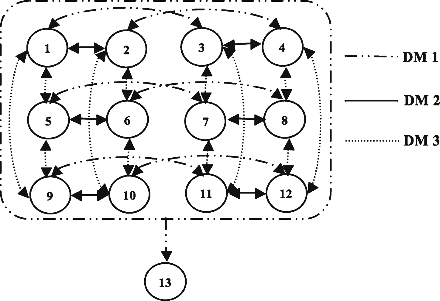
Table 1
Fuzzy stability definitions
| Stability | Definitions |
| Fuzzy Nash Stability (FNash) | A state s is FNash stable for DM i iff |
| Fuzzy General Metarationality (FGMR) | A state s is FGMR stable for DM i iff for every |
| Fuzzy Symmetric Metarationality (FSMR) | A state s is FSMR stable for DM i iff for every |
| Fuzzy Sequentially Stable (FSEQ) | A state s is FSEQ stable for DM i iff for every |
Table 2
DMs and options
| DMs | Options |
| DM 1 | A1: Retain: Keep doing nothing about pollution. |
| A2: Reduce: Reduce pollutant emissions. | |
| A3: Close: Close all polluting factories. | |
| DM 2 | B1: Sanction: Pressure DM 1 to pay the cost of |
| pollution treatment alone,using a variety of necessary sanctions. | |
| DM 3 | C1: Encourage: Provide capital or technological support. |
| C2: Punish: Punish DM 1 if DM 1 does nothing. |
Table 3
Feasible states
| DM | Option | s 1 | s 2 | s 3 | s 4 | s 5 | s 6 | s 7 | s 8 | s 9 | s 10 | s 11 | s 12 | s 13 |
| DM 1 | A1 | Y | Y | N | N | Y | Y | N | N | Y | Y | N | N | - |
| A2 | N | N | Y | Y | N | N | Y | Y | N | N | Y | Y | - | |
| A3 | N | N | N | N | N | N | N | N | N | N | N | N | Y | |
| DM 2 | B1 | N | Y | N | Y | N | Y | N | Y | N | Y | N | Y | - |
| DM 3 | C1 | Y | Y | Y | Y | N | N | N | N | Y | Y | Y | Y | - |
| C2 | N | N | N | N | Y | Y | Y | Y | Y | Y | Y | Y | - |
Table 4
DMs’ preference statements
| DMs | Statements | Descriptions |
| DM 1 | -A3 | Do not select A3 |
| -C2 | DM 3 does not select C2 | |
| A1 IF -C2 | Select A1 if DM 3 does not choose C2 | |
| A2 IF C1&C2 | Select A2 if DM 3 chooses both C1 and C2 | |
| C1&C2 | DM 3 selects C1 and C2 together | |
| -B1 | DM 2 does not select B1 | |
| DM 2 | A3 | DM 1 selects A3 |
| A2 | DM 1 selects A2 | |
| -B1 IF A2 | Do not select B1 if DM 1 chooses A2 | |
| B1 IF A1 | Select B1 if DM 1 chooses A1 | |
| C1&C2 | DM 3 selects both C1 and C2 | |
| C2 | DM 3 selects C2 | |
| DM 3 | A3 | DM 1 selects A3 |
| A2 | DM 1 selects A2 | |
| -B1 | DM 2 does not select B1 | |
| C1&C2 | Select both C1 and C2 | |
| C2 | Select C2 |
Table 5
Fuzzy truth values
| States | DM 1 | DM 2 | DM 3 |
| s 1 | (1, 1, 1, 1, 0, 1) | (0, 0, 1, 0, 0, 0) | (0, 0, 1, 0, 0) |
| s 2 | (1,1,0.65,1,0,0) | (0,0,1,1,0,1) | (0,0,0,0,0) |
| s 3 | (1,0.4,0,1,0,1) | (0,1,1,1,0,) | (0,1,1,0,0) |
| s 4 | (1,0.35,0.25,1,0,0) | (0,1,0,1,0,0) | (0,1,0,0,0) |
| s 5 | (1,0,1,0.2,1,1) | (0,0,1,0,0,1) | (0,0,1,0,1) |
| s 6 | (1,0,1,0,1,0) | (0,0,1,1,0,1) | (0,0,0,0,1) |
| s 7 | (1,0.5,1,0.7,1,1) | (0,1,1,1,0,1) | (0,1,1,0,1) |
| s 8 | (1,0.6,1,1,1,0) | (0,1,0,1,0,1) | (0,1,0,0,1) |
| s 9 | (1,0,1,0,0,1) | (0,0,1,0,1,0) | (0,0,1,1,0) |
| s 10 | (0.85,0,1,0,0,0) | (0,0,1,1,10) | (0,0,0,1,0) |
| s 11 | (1,0,1,1,0,1) | (0,1,1,1,1,0) | (0,1,1,1,0) |
| s 12 | (0.65,0,1,1,0,0) | (0,1,0,1,1,0) | (0,1,0,1,0) |
| s 13 | (0.15,0,1,1,0,1) | (1,0,1,1,0,0) | (1,0,1,0,0) |
Table 6
Fuzzy preference information for DM 1
|
|
Table 7
Crisp preference information for DM 2 and DM 3
| DMs | Preference rankings |
| DM 2 | s 13 ≻ s 11 ≻ s 7 ≻ s 3 ≻ s 12 ≻ s 8 ≻ s 4 ≻ s 10 ≻ s 6 ≻ s 2 ≻ s 9 ≻ s 5 ≻ s 1 |
| DM 3 | s 13 ≻ s 11 ≻ s 7 ≻ s 3 ≻ s 12 ≻ s 8 ≻ s 4 ≻ s 9 ≻ s 5 ≻ s 1 ≻ s 10 ≻ s 6 ≻ s 2 |
Table 8
Fuzzy stability analysis results
| Stability | γ 1 = 0.25, γ 2 = γ 3 = 1.0 | γ 1 = 0.55, γ 2 = γ 3 = 1.0 |
| FNash | s 10, s 11, s 13 | s 11, s 13 |
| FGMR | s 3, s 4, s 7, s 8, s 10, s 11, s 13 | s 3, s 4, s 7, s 8, s 11, s 12, s 13 |
| FSMR | s 3, s 4, s 7, s 8, s 10, s 11, s 13 | s 3, s 4, s 7, s 8, s 11, s 12, s 13 |
| FSEQ | s 10, s 11, s 13 | s 11, s 13 |


