Model and algorithm for resolving regional bus scheduling problems with fuzzy travel times

Wei, Ming; Chen, Xuewu; Sun, Bo; Zhu, Yao-Yao

doi:10.3233/IFS-151972

Model and algorithm for resolving regional bus scheduling problems with fuzzy travel times

Issue title: The fuzzy system and its application in East Asia

Guest editors: Ildar Batyrshin, Dragan S. Pamučar, Paolo Crippa and Feng Liu

Article type: Research Article

Authors: Wei, Ming^{a; b; *} | Chen, Xuewu^b | Sun, Bo^a | Zhu, Yao-Yao^a

Affiliations: [a] School of Transportation, NANTONG University, Nantong, China | [b] Jiangsu Key Laboratory of Urban ITS, Southeast University, Nanjing, China

Correspondence: [*] Corresponding author. Ming Wei, School of Transportation, Nantong University, Nantong, 226019, China. Tel.: +81751304326; Fax: 0513 85012930; [email protected]

Keywords: Urban traffic, regional bus scheduling problem, fuzzy travel time, particle swarm optimization, group search optimization

DOI: 10.3233/IFS-151972

Journal: Journal of Intelligent & Fuzzy Systems, vol. 29, no. 6, pp. 2689-2696, 2015

Published: 2015

Get PDF

Abstract

Regional bus scheduling is necessary to urban public transport that is complicated by the necessity of assigning trips that belong to several routes to buses located at different depots while reducing fleet size and operating costs. Considering the reality of emergencies that may interfere with the ability of vehicles to complete trips on time, it is reasonable to use fuzzy numbers to express uncertain delay times. Based on this idea, this paper proposes a chance-constrained programming model of regional bus scheduling that will reflect additional constraints such as the capacities of related depots and fueling needs. The objective of this paper is to maximize utilization of fleet vehicles. To overcome the defect of premature convergence in the particle swarm optimization algorithm (PSO), an improved PSO is proposed by using an organic fusion with group search optimization. Finally, an example demonstrates the correctness and effectiveness of the model and algorithm.

1Introduction

In contrast to traditional single-depot bus scheduling, the regional bus scheduling problem (RBSP) [5] aims to achieve a unified schedule by sharing vehicle resources across all routes. This is accomplished by inserting deadhead trips between depots to assign trips belonging to several routes to buses located at different depots. Due to the non-uniformity of departure frequency for all routes in a given period, RBSP can significantly reduce operating costs and improve the efficient utilization of vehicles. Bodin and Golden [1] have proven the RBSP is an NP-hard.

Most scholars study RBSP using the optimal scheduling theory, which is divided into network flow [3, 8, 9, 14, 19] and set partitioning [4, 11–13]. Most research into RBSP relies on established travel durations. However, conditions of real traffic environments, such as fluctuations in passenger loads at different time etc., cause deviations between the plan and actual operation, which make practical applications of RBSP difficult to analyze. In general, delays to trip completion are very difficult to predict in advance. Problems in which delay time is assumed to be an uncertain variable are RBSP with uncertain travel times (RBSPUTT). Research into RBSPUTT is rare [6, 7, 11–13]. Huisman and Albert studied RBSPUTT [6, 7] by assuming that future travel time is fixed or predicted in advance. Wei, et al. [11] studied a more realistic RBSPUTT with a stochastic travel time. Wei, et al. [12] proposed a multi-vehicle-type RBSPUTT with a grey travel time, as well as a bi-level programming model for uncertain regional bus scheduling that revealed the overall relationship between a scheduling plan and its procurement scheme [13]. However, these models are typically difficult to solve in practice because of a lack of sufficient reliable historical data to determine the distribution function of the random variable or predict future growth trends.

This paper studies an RBSP with fuzzy travel times (RBSPFTT), which assumes that travel time is an uncertain variable. In combination with the rich experience and knowledge of scheduling staff, fuzzy numbers can represent this type of uncertain information when provided with capacity constraints and other practical factors. In this case, the triangular fuzzy number is used to express the actual travel time; it is then transformed to the corresponding chance-constrained programming model. A new hybrid algorithm based on the fuzzy simulation is proposed to solve the model. Finally, an actual example calculates a bus scheme to test the correctness and effectiveness of the model and algorithm.

2Mathematical model

2.1Mathematical model

– Each trip requires a bus to depart from its depot on time.
– When historical data and expertise are considered, it is possible to use triangular fuzzy numbers to represent certain time delays for each bus trip not completed on time.
– To ensure that a bus does not require refueling during daily operations, it should be fully fueled before or after the work day.

2.2Decision variables

Tdk={x1, x2,…, x|Tdk|} denotes a sequence of trips accomplished in turn by each bus ∀k ∈ V _d, which begins and ends at same depot ∀d ∈ D.

2.3Decision variables

T = {T ₁, T ₂, …, T _|T|} denotes a given set of trips belonging to several routes. Each trip ∀T _i ∈ T requires uninterrupted driving from the starting point sp _{T
_i} at starting time st _{T
_i} to the ending point dp _{T
_i} at ending time et _{T
_i}.

D denotes a given set of depots. For each depot∀d ∈ D, let V _d denote a given set of buses initially located at the depot, and let capacity _d denote the capacity of the depot.

Each vehicle k (∀ k ∈ V _d, ∀ d ∈ D) arrives at the trip ∀xi∈Tdk starting point sp _{x
_i} at the time indicated by txik=etxi-1+ΔTxi-1+time(dpxi-1,spxi). If time (dp _{x
_i-1}, sp _{x
_i}) ≠0, this situation is called a Deadhead Trip (DH Trip). In this situation, time (dp _{x
_i-1}, sp _{x
_i}) denotes the time spent in traveling from the ending point of the trip ∀xi-1∈Tdk to the starting point of the trip ∀xi∈Tdk. ΔT _{x
_i} denotes the fuzzy delay time that prevents a vehicle from accomplishing a trip x _i on time.

a ₀ denotes the weight of number of the buses.

a ₁ denotes the weight of waiting time.

a ₂ denotes the weight of the deadhead time.

Pos {•} denotes the possibility of the case {•}.

|x| denotes the number of elements in the set x.

2.4Objective function equation

(1)

min f¯

2.5Constraint equations

(2)

st. Vp∩Vq=∅ ∀p,q∈D

(3)

∪∀d∈D,∀k∈VdTdk=T

(4)

Tpu∩Tqv=∅ ∀u∈Vp,∀v∈Vq

(5)

|Vd|≤capacityd ∀d∈D

(6)

Pos{etxi-1+time(dpxi-1,spxi)+ΔTxi-1≤stxi}≥α ∀d∈D,∀k∈Vd,∀xi∈Tdk

(7)

Pos{f=a0∑k∈D|Vk|+∑k∈D∑u∈Vk∑xi∈Tku[a1.(stxi-txiu)+a2.time(dpxi-1,spxi)]≥f¯}≥β

The objective function in Equation (1) aims to minimize the number of buses, the total waiting time, and the deadhead time. Equations (2–7) represent the constraints, as follows: Equation (2) ensures that each bus belongs to only one depot; Equation (3) ensures that all trips are successfully completed by all vehicles; Equation (4) expresses that each trip is assigned to exactly one vehicle, and a vehicle cannot simultaneously run two trips; Equation (5) ensures that no more than a given number of backup vehicles are dispatched from each depot; Equation (6) ensures that the possibility of two trips normally accomplished in turn by the same bus in the random environment is at least α; Equation (7) ensures that the confidence level of f¯ representing the maximum value of f is at least β.

3Group particle swarm optimization algorithm for RBSPFTT solution

Particle Swarm Optimization (PSO) [17] is an evolutionary bionic algorithm that simulates flying birds, with advantages including smaller numbers of individuals and simple calculation. PSO performs well in multi-dimensional continuous space optimizations, and provides very rapid local convergence to a stable state. The group search optimization (GSO) [16], recently proposed by S. He and Q.H. Wu, is a novel algorithm based on the social behavior of hunting animals, such as lions and wolves. The GSO performs well in local searches, and can maintain the diversity of the solution to promote the evolution of the population. Each algorithm has advantages and disadvantages. Their homologous natures determine that they should easily integrate with one another; however, current studies involving both algorithms are rare [15].

This paper proposes a Group Particle Swarm Optimization (GPSO) based on a fuzzy simulation to solve RBSPFTT. According to the problem characteristics, the definite scheme solution process is described, and the following terms are defined: particle encoding scheme, constraints handling, and position and velocity correction equation.

3.1Particle code scheme

In GPSO, each individual or potential solution in the swarm is called a particle. Every particle has its own position and velocity, where the position vector can be decoded as a solution to the problem, and the velocity vector is in the direction of particle movement.

The position vector X = (x ₁, x ₂, …, x _|T|) is used to represent a potential solution of RBSPFTT [2, 10], wherein the i-th element is a trip x _i, which differs from other trips in the range 1 - |T|. Furthermore, V = (v ₁, v ₂, …, v _|T|) denotes the velocity vector, where the element v _i is a real number ranging from -|T| - |T|. If ∀x _i-1, x _i ∈ X meets constraint Equation (6), the bus will immediately execute trip x _i after it has accomplished trip x _i-1; otherwise, the two trips would be executed by different buses. Hence, each individual can be decoded into a sequence of trips accomplished by different buses according to Equation (6).

As mentioned above, any individual X satisfies constraints Equations (2–5). Therefore, if the individual X complies with constraints Equations (5–7), it is a feasible solution.

3.2Fitness function

The fitness value, determined by the fitness function, is the standard according to which the merit of each particle position is evaluated. Each particle can be decoded into a set of trips finished by different vehicles. In this paper, Equation (1) is used as the fitness function to assess the quality of any individual. Because all individuals meet constraints Equations (2–4), constraint Equation (5) can be regarded as a penalty function to generate a new fitness function.

(8)

min f¯+A∑∀d∈DMax(|Vd|-capacityd,0)

where A, which is set of a sufficiently large number, denotes the penalty factor. The fitness function, expressed by Equation (8), ensures that an infeasible solution confers great fitness value and will be eliminated in the iteration.

3.3Fuzzy objective function and handling constraints

Constraints Equations (6) and (7) with fuzzy parameters also determine the objective function Equation (8). Because the computer does not deal directly with fuzzy parameters, the fuzzy simulation technology proposed by Wu, et al. [18] can be used to examine its objective function and constraint with respective confidence levels of α and β.

According to the definition of fuzzy number arithmetic for vector ΔT _{x
_i} of a fuzzy delay time in a given decision vector X the establishment of Equation (6) holds if and only if there exists a clear vector ΔTxi0 in the vector ΔT _{x
_i} that satisfies etxi-1+time(dpxi-1, spxi)+ΔTxi0≤stxi and μ(ΔTxi0)≥a, where μ (•) is the membership function of the fuzzy set. That is to say, if etxi-1+time(dpxi-1,spxi)+ΔTxi0≤stxi, which uniformly generates vector ΔTxi0 from fuzzy vector ΔT _{x
_i} in order to satisfy μ(ΔTxi0)≥a, then Equation (6) is established. After a given number N of iterations, if vector ΔTxi0 does not satisfy etxi-1+time(dpxi-1,spxi)+ΔTxi0≤stxi, then the decision vector X is considered to be impossible.

As mentioned above, the specific procedure of fuzzy Equation (6) is as follows:

Step 1: Uniformly generate vector ΔTxi0 from fuzzy vector ΔT _{x
_i} at a horizontal cross-sectional level α;

Step 2: If etxi-1+time(dpxi-1,spxi)+ΔTxi0≤stxi, then the output is “feasible”;

Step 3: Repeat step 1 and 2 N times;

Step 4: Output “infeasible”.

Similarly, the specific procedure of fuzzy Equation (7) is as follows:

Step 1: Set f¯=-∞;

Step 2: Uniformly generate vector ΔTxi0 from fuzzy vector ΔT _{x
_i} at a horizontal cross-sectional level β;

Step 3: If f¯≤f, then f¯=f;

Step 4: Repeat step 2 and 3 N times to calculate f¯;

Step 5: Output f¯.

3.4Formula for modifying position and updating velocity

In PSO, each particle updates itself by tracking the personal extreme value fi*(t) and global extreme value fg*(t) in every iteration. When all particles gather to the same location (that of the current best particle), its velocity approaches zero due to inertia, personal awareness and social consciousness. Each particle will then refuse to search the solution space in other regions.

To address the inadequacies of PSO, a concept derived from GSO is embedded in the search procedure for GPSO; this concept involves a random movement by a small number of rogue particles, wherein each particle generates a random head angle and distance and then moves to this new position. The number of randomly wandering particles is related to the diversity of the population. According to the process described above, the particle updates its velocity and position formula as follows:

(9)

Vi(t+1)=w·Vi(t)+c1·rand·(Xi*(t)-Xi(t))+c2·rand·(Xg*(t)-Xi(t))

(10)

Xi(t+1)={Xi(t)+Vi(t+1),othesXi(t)+liDit(φt+1),rand>σ

where w, c ₁ and c ₂ denote the inertia factor, weight, and global optimal value, respectively;l _i ∈ [0, l _max], φ ^t+1 ∈ [0, θ _max] and Dit(φt+1) denote a random distance, head angle and the vector of the angle, respectively; and rand denotes a random number in the range [0, 1].

Definition 1. σ=1N(N-1)∑i≠j,i,j=1Ncij denotes the population’s diversity where cij={1,fi≠fj0,otherwise.

3.5Algorithm flow

The detailed procedure for GPSO solving RBSPFTT is described as follows.

Step 1: Set the parameters of the algorithm.

Step 2: Let t = 0 and initialize the first generation of particle swarm.

Step 2.1: For each particle, randomly generate its position and velocity vector X _i (0) and V _i (0), and calculate its fitness value f _i (0).

Step 2.2: If Xi*(0)=Xi(0), then fi*(0)=fi(0) to determine the extreme value of each particle.

Step 2.3: Find the global optimal particle fg*(0)=min{f1*(0),……,fn*(0)}.

Step 3: Let t = t+1, and update the current status of the t-th generation swarm.

Step 3.1: For each particle, update its position vector X _i (t) and velocity vector V _i (t), according to Equations (9) and (10).

Step 3.2: Recalculate the fitness value f _i (t). If fi(t)<fi*(t), let fi*(t)=fi(t) and fi*(t)=fi(t). If fi(t)<fg*(t), let fg*(t)=fi(t) and fg*(t)=fi(t).

Step 4: If the termination condition is satisfied, output fg*(t); otherwise return to step 3.

4Analysis of computational examples

A regional bus network is composed of three depots (capacity _d = 15, d = 1, 2, 3) and five routes. Tables 1–4 depict details of the test instance as follows: Tables 1 and 2 demonstrate the basic information and the fixed schedule of these lines; Table 3 depicts the deadhead time information; and Table 4 depicts the fuzzy delay time between two trips. Using a unified model for bus scheduling, a bus company will assign a certain number of vehicles to the three depots to complete a total of 210 trips while minimizing operation costs.

In order to verify the validity of the model and algorithms, the empirical parameters of GPSO are set as follows: the maximum number of iterations is 200, and the number of particles is 50. Let w = 0.75, c ₁ = c ₂ = 1.5, l _max = 5, θ _max = 45o, a ₀ = 500, a ₁ = 1, and a ₂ = 2.5. Matlab was used to program GPSO to solve the RBSPFTT, and the simulation as repeated 50 times at confidence levels α= 1.0 and β= 0.9 on the same computer in order to avoid accidental phenomena. Table 5 indicates the simulation results. There are a total of five solutions. The optimal solution of f is equal to 19,950, the mean is equal to 19,964, and the variance is equal to 28.6. The best solution can be identified at 62% probability, a suboptimal solution can be identified at 22% probability, and the worst solution can be identified at 4% probability. Thus, GPSO can find a satisfactory solution in most cases.

Table 6 demonstrates the best schedule for the regional buses, and Fig. 1 shows the number of vehicles in each parking yard. Each bus follows a predefined trip sequence and is allowed to return to the starting point of the initial trip. That is to say, if a given trip must be assigned to a vehicle, the vehicle must arrive at a fixed time in advance of its starting time. In order to cover all of the trips in a fixed bus time table, 23 buses are required to execute a total of 85 deadhead trips, wherein:

– 9, 9, and 5 vehicles, respectively, are initially located at depots A, B, and C.
– Deadhead trips occur 23, 6, 10, 4, 21, and 21 times between two depots.
– The total working time for all buses is equal to 12,445 min. Their waiting and deadhead times are equal to 4,100 min. and 1,740 min., respectively.

The influence of the two parameters α and β on bus scheduling was also analyzed to study the effect of the fuzzy travel time feature on f. As parameter α decreases and parameter β increases, the number of pairs of feasible trips completed by a vehicle decreases; this leads to a further reduction in the feasible solution space consisting of these pairs, and the sub-solution space containing better solutions is abandoned. Ultimately, the cost of the scheme increases with less uncertainty. However, the scheme is less disturbed by emergencies, and less cost change occurs in the process of a real-time adjustment scheme. The results shown in Fig. 2 are consistent with visual analysis.

In order to verify the validity of the improved algorithms, a case study was calculated 50 times each with GPSO, PSO, and GSO. Figure 3 comparatively analyzes the average simulation results, with the conclusions as follows:

– GPSO, PSO, and GSO require 210, 95, and 390 iterations, respectively, to converge to their optimal solutions. The differences in optimal solutions among them are 2.1% , 2.5% , and 4.6% , respectively. This indicates that GPSO performs better than PSO and GSO in convergence.
– PSO obtains the optimal solution faster than GSO, but it easily converges to local optima. Hence, GPSO, which combines the advantages of the other two algorithms, can perform thermal simulations effectively. By judging the degree of prematurity to maintain swarm diversity, GPSO can not only yield a suboptimal solution quickly, but also jump from local optimization solutions by controlling the search space of particles. This indicates that GPSO performs more robustly than PSO and GSO.

5Conclusions

The primary contribution of this paper is to propose a chance-constrained programming model for regional bus scheduling with fuzzy travel times. Compared to existing studies on RBSPUTT with random or grey travel times, the proposed model can avoid the defect of requiring a large amount of traffic data to determine the distribution function of uncertain travel times, making it easier to optimally solve in practice. The test case analyzed the influence of the fuzzy feature of travel time on bus scheduling, and results indicate that the scheme with less fuzziness of travel time is less disturbed by emergencies and has less cost change in a real-time adjustment scheme.

This paper also contributes to the design of a new hybrid GPSO algorithm, which combines the advantages of both PSO and GSO by embedding the concept of a small portion of particles to take a random walk out of the group into GSO, as occurs in the search procedure for PSO. The simulation indicates that, compared to PSO and GSO in convergence and robustness of the algorithm, GPSO can not only converge to a suboptimal solution quickly, but also jump from a local optimization solution by controlling the search space of particles.

Acknowledgments

This research was supported by the Major State Basic Research Development Program (973 program)(No.2012CB725402),the National Natural Science Foundation of China (Nos. 61503201 and 51178109), China Postdoctoral Science Foundation (No. 2013M540408), University Science Research Project of Jiangsu Province (Nos. 13KJB580008 and 15KJB580011), the Nantong Science and Technology Program (No. BK2014059). This support is gratefully acknowledged. However, all facts, conclusions, and opinions expressed here are solely the responsibility of the authors. The authors thank the anonymous referee for her/his helpful comments.

References

1	Bertossi AA, Carraresi P (1987) On some matching problems arising in vehicle scheduling models Networks 17: 271 281
2	Hosseinabadi AAR (2014) GELS-GA: Hybrid metaheuristic algorithm for solving multiple traveling salesman problem The 14th IEEE ISDA 76 81
3	Haghani A, Banihashemi M (2002) Heuristic approaches for solving large-scale bus transit vehicle scheduling problem with route time constraints Transportation Research 36: 309 333
4	Ribeiro CC, Soumis FA (1994) Column generation approach to the multiple-depot vehicle scheduling problem Operations Research 42: 41 52
5	Wang DY, Zang XY, Wang HX (2008) Research on situation and developing trend for optimization theory and method of public transit vehicle scheduling problem Journal of Beijing Jiaotong University 32: 3 42 47
6	Huisman D, Freling R, Wagelmans APM (2004) A robust solution approach to the dynamic vehicle and crew scheduling problem Transportation Science 38: 447 458
7	Huisman D, Freling R, Wagelmans APM (2006) A solution approach for dynamic vehicle and crew scheduling European Journal of Operational Research 172: 453 471
8	Wang HX, Shen JS (2007) Heuristic approaches for solving transit vehicle scheduling problem with route and fueling time constraints Applied Mathematics and Computation 190: 1237 1249
9	Li JQ, Mirchandani PB, Borenstein DA (2009) Lagrangian heuristic for the real-time vehicle rescheduling problem Transportation Research Part E 23: 419 433
10	He JJ, Zhang K (2015) A hybrid distribution algorithm based on membrane computing for solving the multi-objective multiple traveling salesman problem Fundamental Information 136: 3 199 208
11	Wei M, Jin WZ, Sun B (2011) Model and algorithm for regional bus scheduling with stochastic travel time Journal of Highway and Transportation Research and Development 28: 10 151 156
12	Wei M, Jin WZ, Sun B (2012) Model and algorithm for regional bus scheduling with grey travel time Journal of Transportation Systems Engineering and Information Technology 12: 0 134 151
13	Wei M, Sun B, Jin WZ (2013) Bi-level programming model for uncertain regional bus scheduling problem Journal of Transportation Systems Engineering and Information Technology 12: 2 1 8
14	Kliewer N, Mellouli T, Suhl LA (2006) Time space network based exact optimization model for multi-depot bus scheduling Eurpoean Journal of Operational Research 175: 1616 1627
15	Wu QD, Kang Q, Wang L, Lu JS (2001) An Introduction to Natural Computation Shanghai Shanghai Science and Technology Press
16	He S, Wu H, Saunders JR (2009) Group search optimizer: An optimization algorithm inspired by animal searching behavior IEEE Transactions on Evolutionary Computation 33: 5 973 1001
17	Xie XF, Zhang WJ, Yang ZL (2003) Overview of particle swarm optimization Control and Decision 18: 2 129 135
18	Liu YK, Wang SM (2006) Fuzzy Stochastic Optimization Theory China Agricultural University Press Beijing
19	Liu ZG, Shen JS (2007) Regional bus operation bi-level programming model integrating timetabling and vehicle scheduling Systems Engineering Theory & Practice 11: 135 141

Figures and Tables

Fig.1

Number of vehicles in each parking yard between 06:30–21:00.

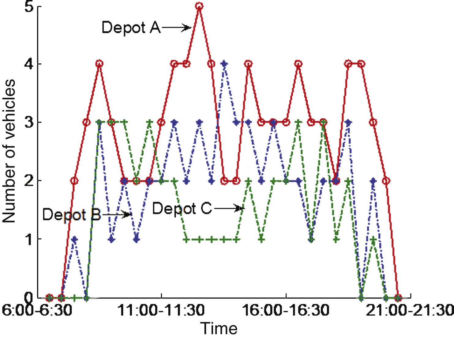
Fig.2

Influence of parameters α and β on bus scheduling.

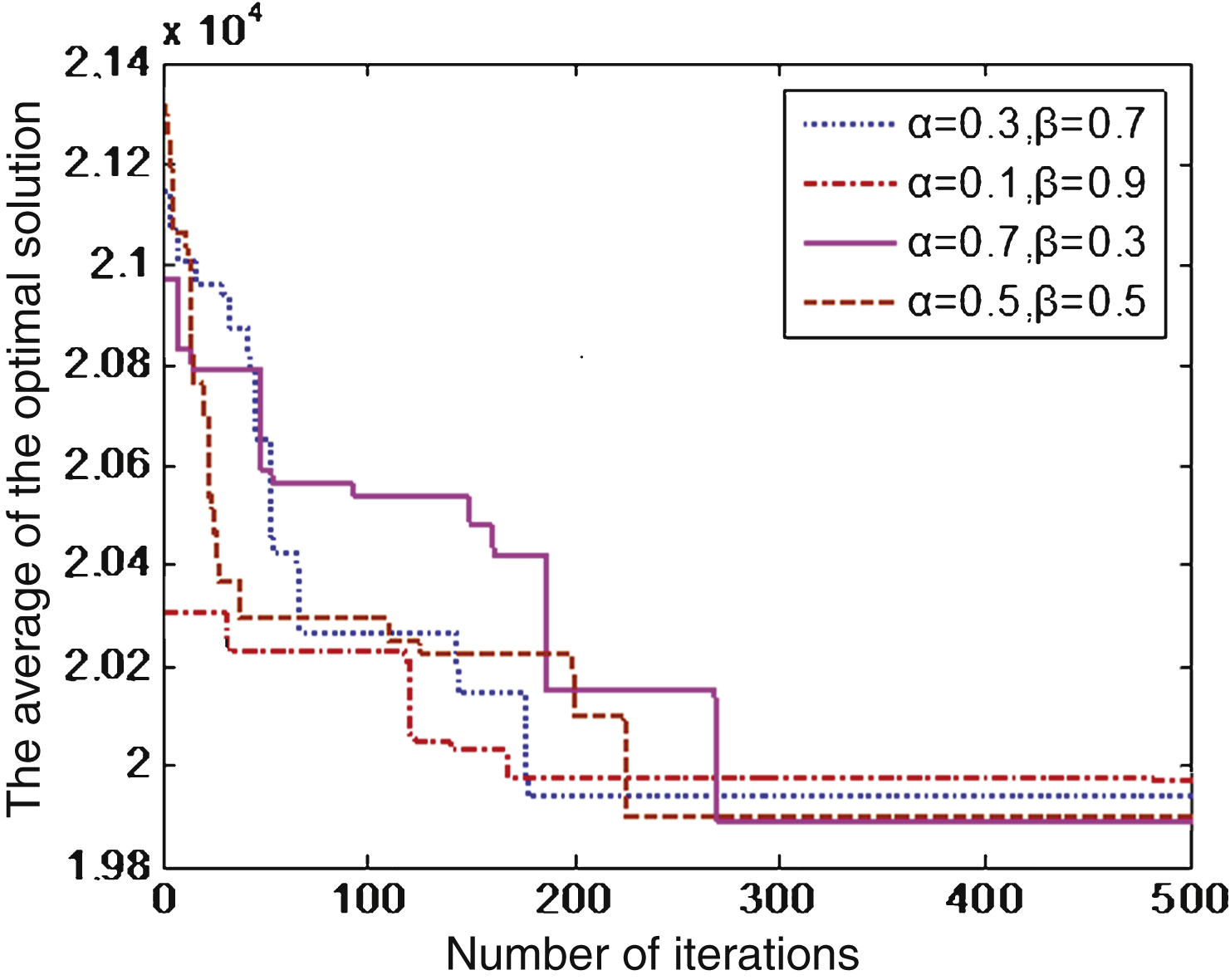
Fig.3

Comparative analysis of three kinds of algorithms.

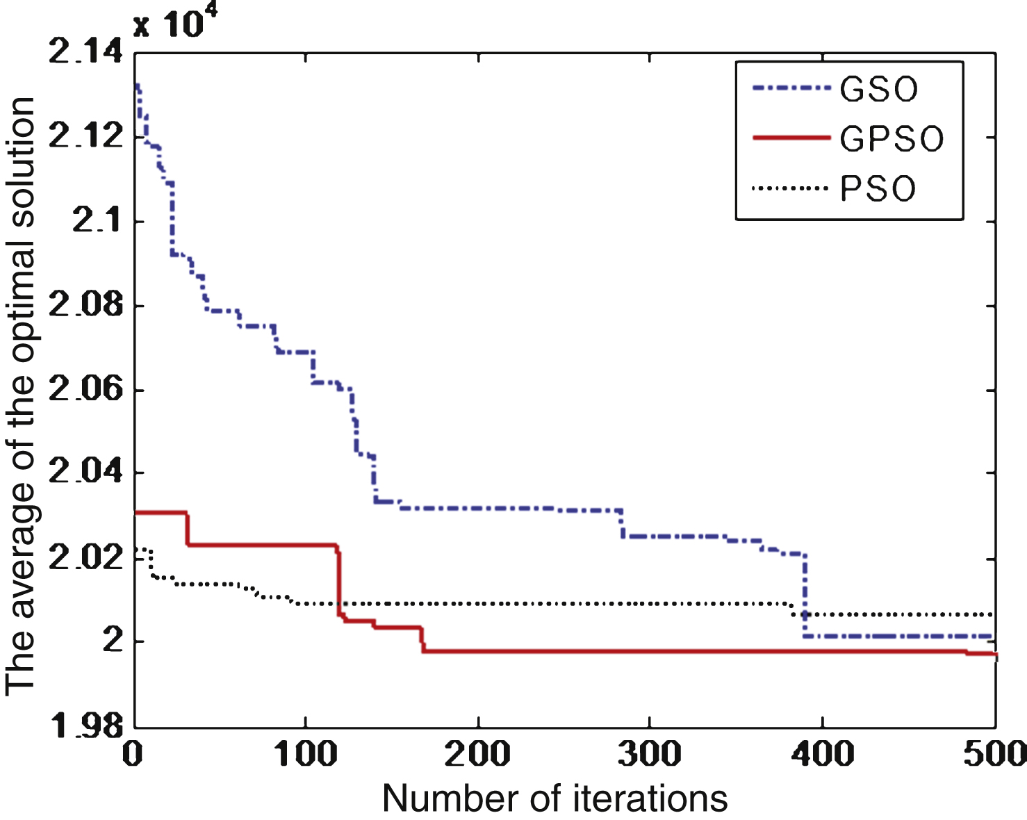
Table 1

Route information

Route	Period	Departure	Start	End	Run
		time (min)	depot	depot	time (min)
1	7:00–20:30	15	A	B	60
2	6:40–20:40	20	B	A	65
3	6:30–21:00	30	A	C	55
4	7:00–20:00	20	C	A	60
5	6:45–20:25	20	B	C	65

Table 2

Timetable of route information

Trip	Departure	Route	Trip	Departure	Route
	time			time
1	7:00	1	…	…	3
…	…	1	128	21:00	3
55	20:30	1	129	7:00	4
56	6:40	2	…	…	4
…	…	2	168	20:00	4
98	20:40	2	169	6:45	5
99	6:30	3	…	…	5
100	7:00	3	210	20:25	5

Table 3

Deadhead time information

Start	End	Deadhead	Start	End	Deadhead
depot	depot	time (min)	depot	depot	time (min)
A	B	20	C	A	20
B	A	25	B	C	25
A	C	15	C	B	20

Table 4

Some fuzzy delay time between trips

Trip	Delay	Trip	Delay	Trip	Delay
	time (min)		time (min)		time (min)
8	(23,29,33)	118	(27,32,34)	159	(25,27,37)
21	(24,28,35)	120	(21,30,36)	162	(23,30,36)
24	(30,36,39)	124	(26,31,37)	163	(24,28,37)
31	(21,22,26)	152	(31,32,38)	166	(20,32,39)
42	(20,26,29)	153	(22,25,34)	171	(20,24,25)
92	(30,32,35)	155	(26,28,33)	193	(25,30,37)
99	(29,33,35)	158	(37,39,40)	208	(21,31,38)

Table 5

Results of 50 simulations

Solution	Objective	Waiting	Deadhead	Probability
type	function	time (min)	time(min)
Best solution	19,950	4100	1740	62%
Suboptimal solution	19.975	4090	1765	22%
Worst solution	20,015	4065	1785	4%

Table 6

Results of bus arrangements

No.	Sequence case of each bus completing the trip	Time (min)
		Traveling	Waiting	Deadhead
1	A-6-64-DH-68-21-191-154-40-202-166-A	540	137	20
2	C-134-DH-179-DH-187-DH-80-37-200-DH-123-54-DH-C	485	170	125
3	B-58-DH-135-14-70-26-DH-32-196-161-124-DH-B	530	185	60
4	B-172-136-16-186-150-DH-195-160-48-DH-55-B	555	225	45
5	B-57-102-140-20-76-115-DH-36-201-165-126-DH-B	580	235	40
6	C-131-12-DH-19-188-152-119-DH-122-DH-52-DH-C	475	213	90
7	A-3-63-106-141-23-83-41-203-DH-96-128-DH-A	580	265	40
8	C-132-104-DH-67-110-DH-114-DH-86-44-206-C	460	210	60
9	B-171-DH-177-143-112-DH-30-82-38-89-51-98-DH-B	590	197	60
10	A-101-DH-176-DH-15-185-148-31-197-DH-46-DH-167-A	550	133	85
11	A-2-DH-10-181-145-DH-77-118-DH-45-207-DH-A	480	219	65
12	A-5-65-108-DH-73-28-81-DH-157-43-DH-50-DH-A	520	155	85
13	C-130-7-66-18-74-DH-78-116-DH-85-DH-204-DH-209-C	585	165	80
14	B-59-9-DH-107-144-DH-189-156-DH-88-DH-94-DH-B	465	205	105
15	B-56-DH-60-11-69-111-149-34-199-DH-92-DH-B	520	215	60
16	B-170-DH-62-DH-180-DH-22-190-153-39-90-49-210-DH-B	610	171	80
17	A-1-61-DH-178-DH-71-DH-75-29-DH-117-159-47-208-DH-A	590	128	105
18	A-100-DH-103-137-DH-183-DH-25-192-155-121-DH-205-168-A	600	132	80
19	A-4-175-139-109-DH-27-DH-33-84-42-93-53-DH-A	590	134	70
20	B-173-138-17-72-113-DH-193-158-DH-164-DH-97-DH-B	535	132	75
21	C-129-DH-133-105-DH-182-146-DH-79-35-87-DH-91-DH-95-DH-C	580	140	110
22	B-169-DH-174-DH-13-184-147-DH-151-DH-198-162-125-DH-B	555	161	95
23	A-99-DH-8-DH-142-24-194-DH-120-163-127-DH-A	470	175	85