Fuzzy grey predictor compensated time-varying variable structure controller for solar inverters
Abstract
In this paper, a fuzzy grey predictor (GP) compensated time-varying variable structure controller (TVVSC) is developed and applied to solar inverters. TVVSC can shorten the reaching phase and ensure the sliding mode occurrence from an arbitrary initial state. However, while loading is a severe nonlinear condition, the TVVSC may suffer from chattering and steady-state error problems, thus deteriorating solar inverter performance. A GP is thus devoted to alleviate the chattering when the system uncertainty bounds are overestimated, and to reduce the steady-state error when the system uncertainty bounds are underestimated. However, the GP with a fixed forecasting value causes long rise time or large overshoot of the system response. Thus, fuzzy logic (FL) is applied to obtain flexible forecasting values to improve the system performance. With the proposed controller, the robustness of the solar inverter system can be enhanced, and a high-quality solar inverter sinusoidal output voltage with low voltage harmonics and fast dynamic response can be obtained, even under nonlinear loading. The theoretical analysis, design procedure, computer simulations, and digital signal processing (DSP)-based experimental implementation for solar inverters are presented to verify the efficacy of the proposed controller.
1Introduction
In recent years, solar inverters have gained increasing attention, and been broadly used in energy conversion systems [4]. In solar energy systems, the overall performance is dependent upon the static inverter-filter arrangement, which is used to convert a DC voltage into a sinusoidal AC output. The requirements for a high-performance solar inverter must supply a high-quality AC output voltage with low total harmonic distortion (THD), zero steady-state error and a fast dynamic response; these can be obtained by employing feedback control techniques. The linear proportional Integral (PI) controller is typically used. However, the classic PI controlled system can not ensure fast and stable output voltage response [7, 9]. Various control techniques have been proposed, such as wavelet transform technique, deadbeat control, and repetitive control, etc. However, these control techniques are difficult to implement and complex in computation [3, 10, 13]. For robust control systems, the variable structure control (VSC) can be adopted because the VSC is insensitive to systemuncertainties, and provides a fast dynamic response. The controller of the solar inverters is also very popularly designed with VSC; however, the design of the classic VSC with fixed sliding surface is employed, and the sliding mode is attained when the system state reaches and maintains on the intersection of the sliding surface [1, 14]. Thus, the trajectories are sensitive to uncertainties before the sliding mode occurs. To improve such problems, the concept of the TVVSC is introduced. The TVVSC is first chosen to pass arbitrary initial conditions and subsequently moved towards a predetermined sliding surface by means of rotating and/or shifting. By employing the time-varying sliding surface, the system sensitivity to uncertainties is reduced by shortening the reaching phase [8, 12]. However, once a highly nonlinear loading is applied, the TVVSC controlled system is subject to chattering and steady-state error, thus resulting in serious voltage harmonics in the solar inverter output, even deteriorating the solar inverter performance. The grey predictor (GP) has been proposed by Deng, and many applications in a variety of fields have been developed. The grey model is built based on first-order differential equations, and utilizes mathematical approximation to transfer a continuous form into a discrete form. Such a transformation will confront some unconquerable problems, such as limited sampling frequency, sample/hold effects and discretization errors. Use of a difference equation replaces the differential equation to build a grey model that provides a reasonable and exact approach [5, 11]. This paper employs a mathematically simple and computationally efficient GP to alleviate the chattering and steady-state error when the system uncertainties are overestimated or underestimated. Though GP requires several output data to achieve a grey model and to forecast a future value without complex calculation, the GP uses a fixed forecasting value and leads to long rise time or large overshoot of the system response. Fuzzy set theory was introduced in 1965 and has received extensive applications. Fuzzy logic (FL) is thus used to tune the GP flexible forecasting value so as to maintain both a short rise time and a small overshoot of solar inverters system response [2, 6]. By combining FL, GP, and TVVSC, the proposed controller will yield a closed-loop solar inverter with low THD, fast dynamic response, elimination of chatter, and steady-state error reduction under various types of loads. Simulation and experimental results are demonstrated to verify the performance of the proposedcontroller.
2Solar inverter control design
A representative single-phase solar inverter is shown in Fig. 1, with a DC power supply Vdc, resistance load R, PWM full-bridge inverter and L-C filter. The proposed controller is used to design a 1KW 60 Hz solar inverter.
The L - C filter and R are considered to be a plant system, and the dynamics with state variables are expressed as:
(1)
The model system is given by the sinusoidal function with 60 Hz.
(2)
By defining e1 = xm1 - xp1, subtracting Equation (1) from Equation (2), the error differential equation yields:
(3)
(4)
Then, the time-varying sliding surface is selected as:
(5)
Taking the derivative of σ yields:
(6)
Define
(7)
The equivalent control ue, which can determine the dynamic of the system on the sliding surface is derived as:
(8)
Substituting up = ue into Equation (8) yields:
(9)
When in sliding action:
(10)
Substituting Equation (10) into Equation (9) yields:
(11)
The system performance can be ensured despite the existence of the uncertain system dynamics. The sliding control us is designed as follows:
(12)
Inserting Equation (12) in
Notice that if a highly nonlinear loading is connected to solar inverter output, the chattering and steady-state error will occur. Thus, we employ the GP with GM(2,1) model to eliminate the chattering and steady-state error. The GP modeling steps are described below.
Step 1. Gather the original sample data sequence
(13)
Step 2. Mapping generating operation (MGO).
The data sequence of the system may be positive or negative. The MGO maps the negative data to the relative positive data.
(14)
Step 3. Take accumulated generating operation (AGO) for
(15)
Step 4. Build the GM(2,1) model.
The linear difference equation grey prediction model is established as:
(16)
The, Equation (16) is rewritten as the following matrix:
(17)
Let k = 1, 2, . . . , n-2 and suppose
(18)
Let
(19)
The roots to satisfy Equation (19) are given as:
(20)
If ξ1 ≠ ξ2, the solution of the prediction model of the second-order difference equation can be expressed as:
(21)
If ξ1 = ξ2, the solution of the prediction model of the second-order difference equation can be expressed as:
(22)
If ξ1 and ξ2 are complex conjugate, the solution of the prediction model of the second-order difference equation can be expressed as:
(23)
Step 5. Take inverse accumulated generating operation (IAGO).
(24)
Step 6. Inverse mapping generating operation (IMGO).
Applying IMGO to
(25)
Then, the control law of Equation (7) is restated as:
(26)
(27)
(28)
It is worth noting that the above-mentioned GP uses a fixed forecasting value, and may cause long rise time or large overshoot of the system response. To solve such a problem, FL is introduced to finely tune the GP forecasting value, thus enhancing the system robustness. The operation of fuzzy tuning GP forecasting value is illustrated as follows. Let the predicted error and the change of the predicted error at the kth-step ahead be
R1: If
R2: If
⋮
R49: If
3Simulation and experimental results
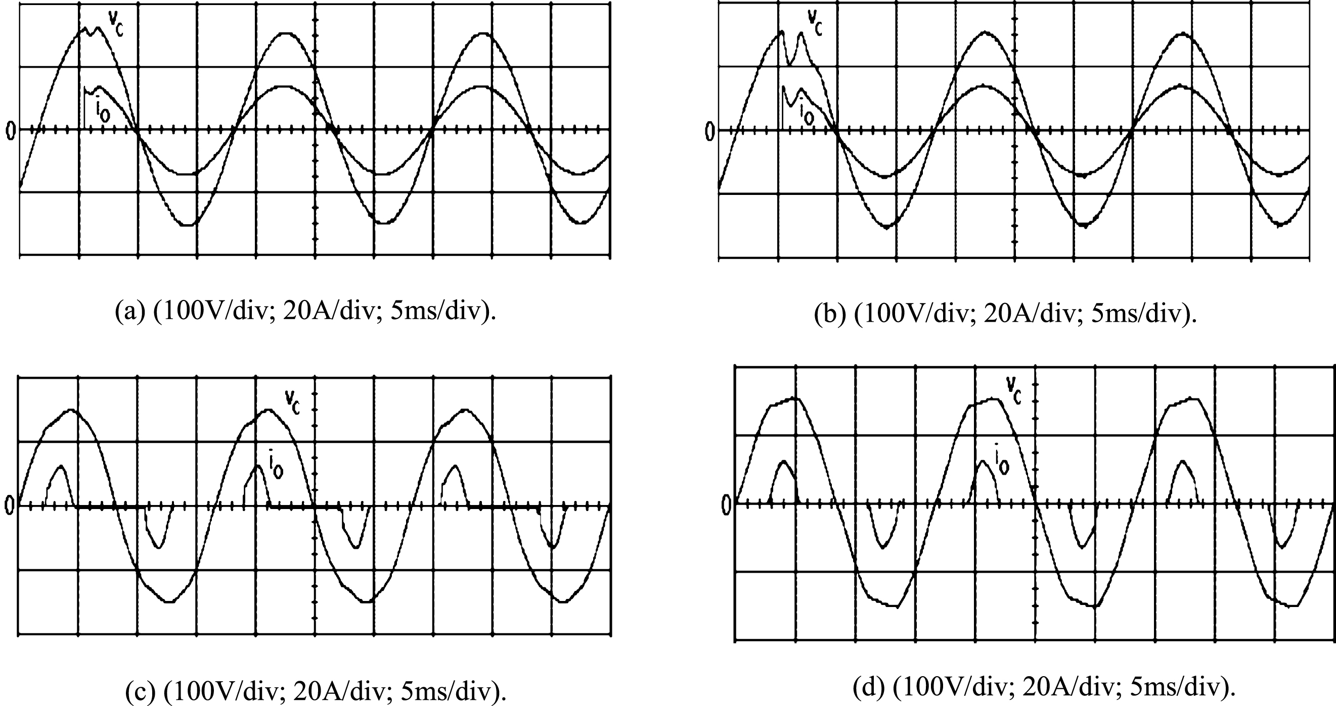
The system parameters of the solar inverter are given as follows: DC-bus voltage, V dc =200 V; switching frequency, fs = 15 kHz; output voltage and frequency, v c = 110 Vrms, f = 60 Hz; rated resistive load, R = 12Ω; filter inductor, L = 1.5 mH; filter capacitor, C = 15μF. Figure 2(a) depicts the simulated transient response with the load changing from no load to full load at t = 0.0208 s for the proposed controller. The transient response of the proposed controller is very fast, taking only a few sampling intervals to reach steady-state. On the contrary, the simulated waveforms shown in Fig. 2(b) with classic VSC indicates a significant voltage sag. A simulated performance testing, shown in Fig. 2(c) is achieved by applying a nonlinear load consisting of a diode bridge, a capacitor (100μF) and a resistive load (60Ω). The simulated % THD computed in the output voltage is 1.13% ; The AC voltage is still satisfactory, and good behavior of the inverter is also obtained in this critical condition. However, under the same rectifier loading obtained using the classic VSC, shown in Fig. 2(d), exhibits a high simulated % THD output voltage (% THD of output voltage is equal to 8.01%). Figure 3(a) displays the experimental output voltage and the load current with the proposed controller under a load step change from open circuit to R = 12Ω. A rapid recovery of the steady-state response can be obtained. However, the experimental waveform with the classic VSC, shown in Fig. 3(b), demonstrates poor voltage compensation, especially at the firing angle. Additionally, the majority of sensitive loads are rectifier loads. When the diodes are conducting, the inverter is exposed to a large filter capacitor, and when the diodes are not conducting, the inverter is practically in no load condition. Therefore, the controller must correctly regulate output voltage with minimum distortion. Figure 3(c) shows the experimental output voltage and the load current with the proposed controller when the inverter is loaded with a full-wave rectifier followed by a 100μF capacitor in parallel with a 60Ω resistor; the experimental % THD is close to 1.17% , which indicates good inverter performance. On the contrary, Fig. 3(d) with the classic VSC under the same test condition exhibits a high experimental voltage % THD of 7.42% .
4Conclusions
A fuzzy GP-compensated TVVSC has been proposed to improve the tracking behaviors of solar inverters. The TVVSC can shorten the reaching phase, thus enhancing the robustness of the system. However, with the application of a highly nonlinear loading, chattering and steady-state error occur. For high tracking accuracy, the GP is used to eliminate the chattering and steady-state error, which are produced by TVVSC. Additionally, FL is added to GP to tune the forecasting value, thus enhancing the system robustness and speed. Simulation and experimental results indicate that low THD, fast transient response, the elimination of the chattering, and the reduction of the steady-state error are obtained by the proposed controlled solar inverter under both steady-state loading and transient loading.
Acknowledgments
This work was supported by the Ministry of Science and Technology of Taiwan, R.O.C., under contract number MOST104-2221-E-214-011.
References
1 | Abrishamifar A, Ahmad AA, Mohamadian M (2012) Fixed switching frequency sliding mode control for single-phase unipolar inverters IEEE Trans on Power Electronics 27: 5 2507 2514 |
2 | Syropoulos A (2014) Theory of Fuzzy Computation Springer-Verlag New York |
3 | Chen D, Zhang JM, Qian ZM (2013) An improved repetitive control scheme for grid-connected inverter with frequency-adaptive capability IEEE Trans. on Industrial Electronics 60: 2 814 823 |
4 | Luo FL, Ye H (2010) Power electronics: Advanced conversion technologies CRC Press |
5 | Li GD, Masuda S, Yamaguchi D, Nagai M, Wang CH (2010) An improved grey dynamic GM(2,1) model International Journal of Computer Mathematics 87: 7 1617 1629 |
6 | Abu-Rub H, Iqbal A, MoinAhmed S, Peng FZ, Li Y, Ge BM (2013) Quasi-Z-source inverter-based photovoltaic generation system with maximum power tracking control using ANFIS IEEE Trans on Sustainable Energy 4: 1 11 20 |
7 | Rasoanarivo I, Brechet S, Battiston A, Nahid-Mobarakeh B (2012) Behavioral analysis of a boost converter with high performance source filter and a fractional-order PID controller Proc IEEE Int Conf Industry Applications Society Annual Meeting 1 6 |
8 | Geng J, Sheng YZ, Liu XD (2013) Second-order time-varying sliding mode control for reentry vehicle International Journal of Intelligent Computing and Cybernetics 6: 3 272 295 |
9 | Rebeiro RS, Uddin MN (2012) Performance analysis of an FLC-based online adaptation of both hysteresis and PI controllers for IPMSM drive IEEE Trans on Industry Applications 48: 1 12 19 |
10 | Saleh SA, Rahman MA (2011) Experimental performances of the single-phase wavelet-modulated inverter IEEE Trans on Power Electronics 26: 9 2650 2661 |
11 | Liu S, Lin Y (2010) Advances in Grey Systems Research Heidelberg, Berlin Springer-Verlag |
12 | Tokat S, Eksin I, Guzelkaya M (2009) Linear time-varying sliding surface design based on co-ordinate transformation for high-order systems Transactions of the Institute of Measurement and Control 31: 1 51 70 |
13 | Zhang XG, Zhang WJ, Chen JM, Xu DG (2014) Deadbeat control strategy of circulating currents in parallel connection system of three-phase PWM converter IEEE Trans on Energy Conversion 29: 2 406 417 |
14 | Hao X, Yang X, Liu T, Huang L, Chen WJ (2013) A sliding-mode controller with multiresonant sliding surface for single-phase grid-connected VSI with an LCL filter IEEE Trans on Power Electronics 28: 5 2259 2268 |
Figures and Tables
Fig.1
Block diagram of solar inverter.
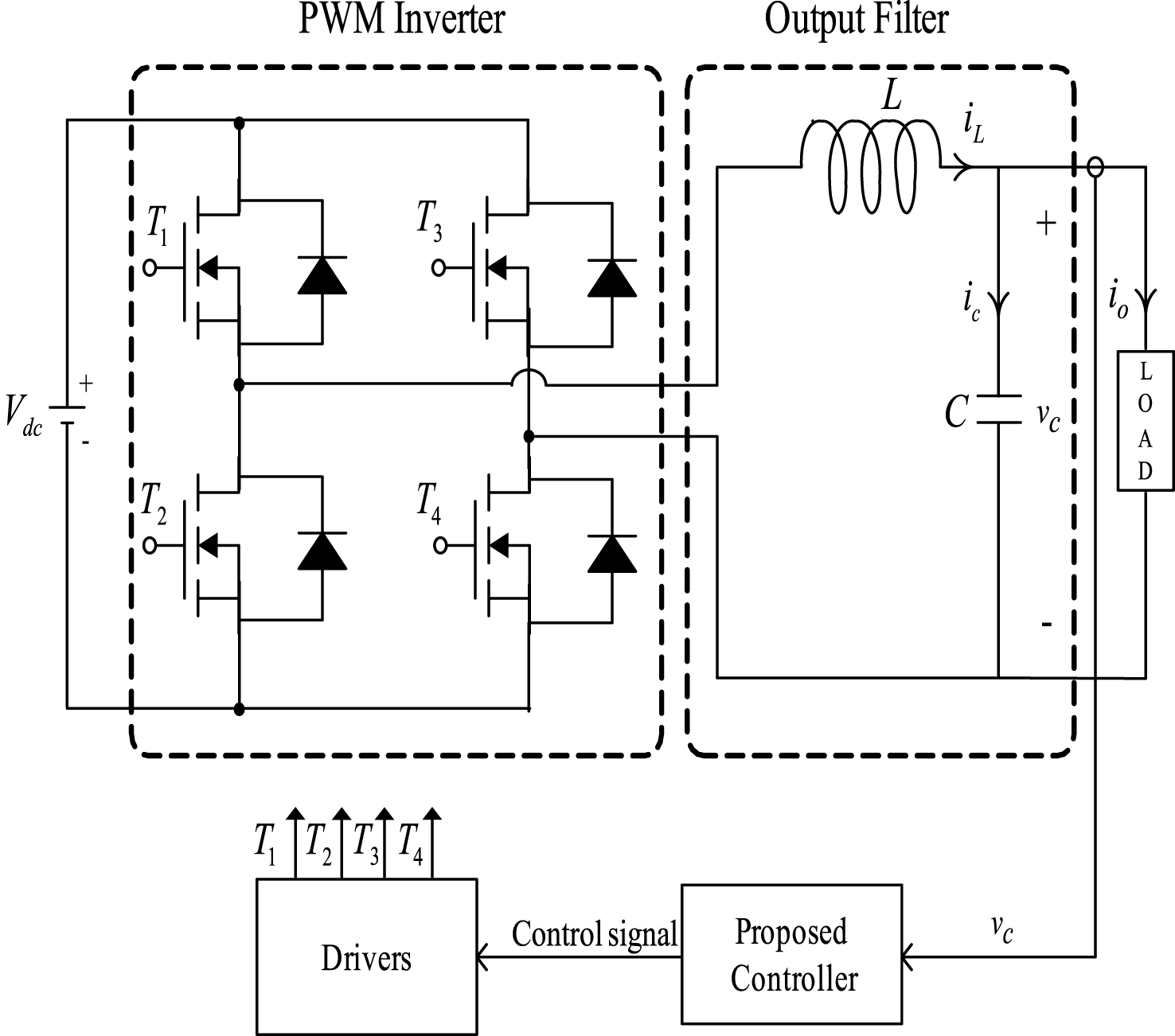
Fig.2
Depicts the simulation results of output voltage and load current under (a) step change in load with the proposed controller; (b) step change in load with classic VSC; (c) rectifier load with proposed controller; (d) rectifier load with classic VSC.
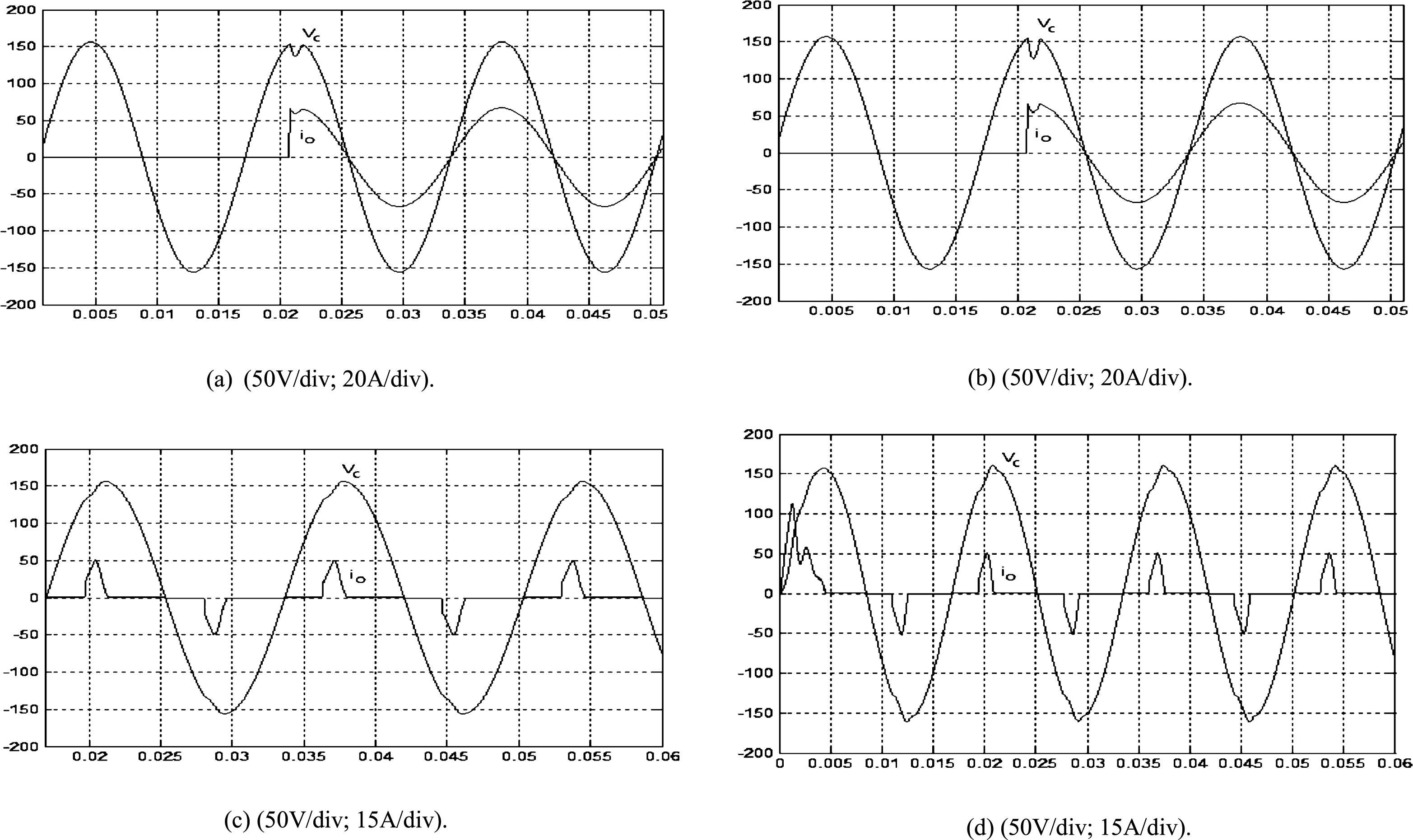
Fig.3
Experimental waveforms under (a) step change in load with the proposed controller; (b) step change in load with classic VSC; (c) rectifier load with proposed controller; (d) rectifier load with classic VSC.