
A photovoltaic array simulator based on current feedback fuzzy PID control
Abstract
A photovoltaic array simulator is designed based on a Buck DC converter with a fuzzy PID control algorithm to account for current feedback. The conventional PID controller cannot self-tune the parameters, therefore the new algorithm uses a fuzzy controller to solve the problem. The difference between the reference current and the real-time feedback current of the Buck converter and its rate of change are regarded as two input variables of the fuzzy controller. The fuzzy controller outputs the adjustment quantities, which are then used to adjust the PID parameters. Next, the duty cycle of the electronic power switch is adjusted by a closed-loop fuzzy PID algorithm to make the output current of the simulator work at the anticipated point of the photovoltaic array on the I-V characteristic curve and realize the simulation of photovoltaic characteristics. Results of the simulation and experiment indicate that the proposed fuzzy PID control simulator can not only accurately simulate the static output characteristics of a photovoltaic cell, but can also rapidly realize the dynamic characteristics when the load or the external environment changes. The approximate error was less than 3.6% , the overshoot was less than 3.5% , the ripple coefficient was less than 3% , and the tracking time was approximately 0.3s. The fuzzy PID control simulator can work well as PV array experiment equipment for the research and development of photovoltaic systems.
1Introduction
In general, a photovoltaic (PV) power generation system (PVPGS) is primarily composed of PV cells, controllers, power converters and batteries. Utilizing the PV cells to conduct PVPGS experiments is often restricted by seasons and weather, especially at night, as when the environment changes the PV cells cannot maintain a stable output test. Moreover, the PV cells greatly increase the cost of testing. Therefore, using PV cells to test the performance of PVPGS induces major inconvenience. As a consequence, the PV simulator [4, 10, 11] is an ideal solution to simulate PV cell output I-V characteristics under different temperatures and illumination conditions, free from climate change influence, and provide favorable conditions for the performance test of PVPGS. Currently, depending on the different types of simulators, it may be an analog simulator, digital simulator or a mixed simulator. A digital simulator [7, 9] combines the power electronics technology and real-time control technology, presents high precision and controllable output characteristics, and simulates a large-capacity power system. Therefore, a digital simulator is well suited to the research and development of the PVPGS, and has been extensively studied [14]. Digital simulators use algorithms such as the secant method, numerical iteration method and point by point approximation (PPA) method. Among these, the secant method requires much computation, as it requires the solving of complex transcendental equations. The numerical iteration method and PPA are closely related to the step size; the system will produce greater oscillation if the step size used is too large. To achieve a stable output, the step size must be small, but will then induce a slow dynamic response.
Fuzzy logic [1, 5, 6, 16] plays an important role in accounting for uncertainty when making decisions in control systems. Until 2013, all studies on fuzzy derivative, fuzzy integral and fuzzy differential equations had been conducted based on type-1 fuzzy sets (T1FSs). Mehran Mazandareni define type-2 fuzzy fractional derivatives and present type-2 fuzzy fractional differential equations (T2FFDEs) [12, 13]. Housheng Zhang designed a simulator using a dual-loop control with a PI regulator [8], which can enhance the system performance. However, in case of a controlled system that is strongly time-varying and nonlinear, a pre-set PI parameter cannot meet its requirements. As a consequence, this paper presents a fuzzy PID control algorithm with a BUCK circuit used as a power converter. In the proposed method, the output current i and voltage u of the BUCK circuit are sampled in real-time. The voltage sampling value is substituted into the PV cell engineering mathematical model to generate a reference current iref. The diffrence e = iref-i and its rate of change de/dt are used as two input variables of the fuzzy controller. The outputs of the fuzzy controller are used to modify the PID parameters, and then control the BUCK power converter using a PWM method output corresponding current and voltage according to the I–V curve of PV cells. The operating point of the simulator will be made to match the output characteristics of the PV cells. The block diagram of the digital simulator is shown inFig. 1.
A fuzzy PID PV simulator consists of a BUCK converter and a controller based on TMS320F2812. The controller generates a PWM control signal to control the converter according to the PV cell I–V curve. Simulation and experiment results indicate that the simulator possesses a fast dynamic response and stable output characteristic under different conditions, with an overshoot less than 3.5% , a steady-state error less than 3.6% , a ripple factor less than 3% , and tracking time less than 0.3s.
2Output characteristic of PV cell
The I–V output characteristics [15] of a PV cell are nonlinear, and are affected by the illumination intensity and condition temperature, as shown in Fig. 2. The current-voltage curve of a PV cell at 25°C and 50°C are respectively shown in Fig. 2(a) and (b).
Simplified mathematical models to describe the output characteristics of PV cells generally use the short-circuit current I sc , open circuit voltage V oc , the maximum power point current I m and the maximum power point voltage V m under standard test conditions (S ref = 1000 W/m2, T ref = 25°C).
(1)
(2)
(3)
When the illumination intensity S and temperature T are non-standard test conditions, I sc, V oc, I m, V m and the coefficients C 1, and C 2 will change. Setting ΔS, ΔT as the variation from the standard test conditions of illumination and temperature respectively, four basic parameters can be calculated by utilizing the following formula, known as the PV cell engineering mathematical model:
(4)
(5)
(6)
(7)
Replacing I
sc, V
oc, I
m and V
m in Formulas (1) through (3) with
3Fuzzy PID controller
3.1Control objective of the simulator
When the illumination intensity and temperature remain constant, the PV cell demonstrates a unique I-Vcharacteristic curve. Corresponding to a determined load R, I-V curves of load must meet the output I-V curve of the PV cells at a point; for example, if the load changes from R 2 to R 1, the intersection must change from point E to point C (R 2 is less than R 1). The control target of the simulator is to allow the output characteristic of the converter run on the point C from point E by controlling the duty cycle d of the DC-DC circuit, as shown in Fig. 3.
3.2Design of fuzzy PID controller
Due to its nonlinearity, it is very difficult to describe the characteristics of PV cells using an accurate mathematical model. As the PV generation system has strong uncertainty, a fuzzy PID control is used to resolve these problems and realize the tracking of the output current. The structure diagram of a two-dimensional fuzzy PID controller is shown in Fig. 4. In Fig. 4(a), V n and I n are the output voltage and current of the simulator in sampling time n, respectively. V n is substituted into the above engineering mathematical model, which is composed of the Formulas (1) through (7), to calculate the theoretical current I ref of PC cell. Set e (n) is the error of I ref and I n, and ec(n) is the rate of change of e (n). E (n) and EC (n) are the current error and current error variances respectively quantified by the quantized factor K e and K ec, and serve as two input variables of the fuzzy controller. The variable quantities (ΔKp, ΔKi, ΔKd) corresponding to the proportional, differential and integral coefficient in the PID controller can be obtained by means of fuzzy inference, defuzzification and range conversion (Ka, Kb, Kc). The duty cycle adjustment value ΔD of the DC / DC converter is calculated by the PID controller, and a new duty cycle D(n) = D(n-1)+ΔD can be obtained. The converter operating state is adjusted according to the duty cycle D to make the output operating point of the simulator run on the I-V characteristic curve of the PV cell at point C, as shown in Fig. 3.
3.3Fuzzy algorithm design
The universal ranges of input and output variables are restricted to {3, 2, 1, 0, 1, 2, 3}; fuzzy subsets {NB, NM, NS, ZO, PS, PM, PB} correspond to negative big, negative middle, negative small, zero, positive small, positive middle, and positive big, respectively. The membership functions of input E, EC and output ΔKp/ΔKi/ΔKd adopt the isosceles triangle function, as shown in Fig. 5.
In addition, in order to ensure the input linguistic variance E and EC in its universal range, the quantitative factors Ke and Kec are used respectively before the E and EC are inputted to the fuzzy controller. The process of determining the fuzzy quantization factors is detailed below.
As shown in Fig. 4, the following equation can be obtained Δe (n) = Iref (n) - I (n) , ec (n) = e (n) - e (n - 1) , e (n) max = Isctake Ke = 3/Isc. Then:
(8)
(9)
(10)
(11)
Which can simplify to:
(12)
Since VB > VA, a minimum value 1v of each voltage variation is set in the program. Thus, (VB > VA) min = 1, the maximum value of VB is approximately equal to the open circuit voltage VOC, and the following equation can be obtained from Formula (12):
(13)
Take Kec = 3/ ec(n)max:
(14)
According to the output characteristics of the PV cell and the control objective of the simulator, self-tuning rules of Kp, Ki and Kd follow three basic principles:
1) When the error E is large, in order to accelerate the response speed of system and prevent system loss of control due to the large deviation, system should adopt the larger Kp and smaller Kd. In order to protect the system from a large overshoot, the value of the Ki also should be smaller.
2) When the error E and error change rate EC is medium, in order to reduce overshoot of the system and ensure an ideal dynamic response speed, Kp and Kd should be smaller; the value of the Ki is appropriate.
3) When the error E is small, in order to provide a good steady-state performance, the values of Kp and Kishould increase. Simultaneously, in order to avoid oscillation of the output response and consider the anti-jamming performance of the system, Kd should be appropriate. When the EC is small, Kd takes on a larger value; when EC is large, Kd should be smaller. The fuzzy rules of the controller are concluded as shown in Tables 1 through 3.
Finally, using the gravity method of defuzzication, the precise controlled quantity is obtained.
4Main parameters of the simulator test circuit
The basic circuit diagram and experimental platform are shown in Fig. 6. The main circuit of the system is composed of a step-down rectifier circuit, detection circuit, power supply, control circuit and PWM driving circuit. The output voltage of the rectifier circuit is 62∼67 V. The controller uses TMS320F2812 as its core. The parameters of the PV cell at 25°C and an irradiation of 1000 W/m2 are listed in Table 4. The parameters of the fuzzy PID controller are as follows: Ka = 0.1, Kb = 1, Kc = 1, Kp = 0.1; Ki = 50; Kd = 100; Ke and Kec are detailed in Section 3.3.
5Analysis and discussion of simulation and experiment results
5.1Analysis of simulation results
Simulation experiments are conducted using the proposed fuzzy PID algorithm. Figure 7 depicts the tracking waveforms during the system startup process and the load mutation. Figures 8 and 9 depict the tracking performance during illumination intensity change and temperature altering, respectively. In each figure, the load current is shown by a dotted line and the theory current is shown by a solid line.
5.1.1Tracking performances during the system startup process and load mutation
To study the tracking performance of the simulator during the startup process and the load mutation, a simulation under standard test conditions was initically conducted. Figure 7(a) shows the waveforms during the system startup from the initial operating point, at which the load R = 10Ω and then transforms to 16Ω at 0.2s. Figure 7(b) shows the waveforms during the system startup from the initial operating point, at whichwhich the load R = 16Ω and then transforms to 10Ω at 0.2s.
Figure 3 depicts the I-V characteristic curve of the PV cell. If the load R of the simulator is small, the working point is located at a point with higher voltage and lower current. On the contrary, if the load R of the simulator is large, the working point will be a point with higher current and lower voltage. According to the working principle, the dynamic performance of the simulator is related to the difference between the load current and the target point current; a greater difference requires a longer settling time.
Figure 7(a) shows the current tracking waveform for the startup with a small load; the settling time of the startup process is 0.07s, and its tracking time is 0.04s when the load changes from 10Ω to 16Ω at 0.2s.Figure 7(b) shows the current tracking waveform for the startup with a large load; its settling time of the startup process is 0.05s, and its tracking time is 0.1s when the load changes from 16Ω to 10Ω at 0.2s. The entire simulation approximate error is 0.8% , and the ripple coefficient is 0.6% .
5.1.2Simulation under varying illumination intensity
The ambient temperature T = 30°C, load R = 10Ω, and the illumination intensity S mutates at 0.2s from 1000 W/m2 to 800 W/m2. The simulation waveforms are shown in Fig. 8. Figure 8 demonstrates that the tracking time of the simulation is approximately 0.12s, and the steady-state error and ripple factor are approximately 0.8% and 0.6% , respectively. Results indicate that when the weather varies, the fuzzy PID algorithm possesses good dynamic response speed and steady-state accuracy.
5.1.3Simulation under varying temperature
The ambient temperature S = 1000 W/m2, load R = 8Ω, and the temperature T changes at 0.2s from 70°C to 10°C. The simulation waveforms are shown in Fig. 9. Figure 9 indicates that the tracking time of the simulation is approximately 0.08s,with a steady-state error and ripple factor of approximately 1% and 0.6% , respectively. The simulation results indicate that when the weather varies, the fuzzy PID algorithm possesses a preferable dynamic response speed and excellent tracking performance.
5.2Analysis of experiment results
The experiments were conducted on the experimental platform shown in Fig. 6. In this section, three kinds of experiments are proposed and analyzed: (1) System startup process; (2) Dynamic performance with load mutation; (3) Dynamic performance with illumination mutation.
5.2.1Tracking features during the system startup process
Figure 10 shows the waveforms during the startup process of simulations under the following conditions: ambient illumination S = 1100 W/m2, load R = 10Ω, temperature T = 30°. Figure 10(a) shows the waveforms of the proposed fuzzy PID controller, and Fig. 10(b) represents the traditional point-by-point approximation (PPA) method.
According to Fig. 10(a), the tracking time of the proposed fuzzy PID is approximately 200 ms, the steady-state error is approximately 2% and the ripple coefficient is 2.8% . The tracking time of the traditional method is approximately 260 ms, the steady-state error is approximately 3% and the ripple coefficient is 3% , as shown in Fig. 10(b). As a consequence, the fuzzy PID algorithm demonstrates better rapidity and steady-state performance.
5.2.2Dynamic tracking performance with load change
In this section, the dynamic response performance is analyzed when the load changes under the following conditions: ambient illumination S = 1100 W/m2, load R = 10Ω, temperature T = 30°. Figures 11 and 12 represent the waveforms corresponding to the proposed fuzzy PID algorithm and the traditional PPA method, respectively. Figures 11(a) and 12(a) show the waveforms when the load changes from 8Ω to 16Ω. Figures 11(b) and 12(b) show the waveforms when the load changes from 16Ω to 8Ω.
Based on Fig. 11(a), the response time of the fuzzy PID is nearly 180 ms when the load changes from 8Ω to 16Ω; Fig. 11(b) shows that the response time is approximately 320 ms when the load changes from 16Ω to 8Ω, and the steady-state errors under the two conditions are approximately 2.2% . According to Fig. 12(a), the response time of the PPA method is approximately 200 ms when the load changes from 8Ω to 16Ω,; Fig. 12(b) shows that the response time is approximately 320 ms when the load changes from 16Ω to 8Ω, and the steady-state errors under the two conditions are approximately 2.6% .
5.2.3Dynamic tracking performance with illumination change
This experiment verifies the dynamic response performance when the illumination intensity changes from 1200 W/m2 to 800 W/m2 under the following conditions: ambient temperature T = 30°, load R = 11Ω. According to Fig. 13(a), the tracking time of the fuzzy PID is approximately 110 ms when the illumination intensity changes, and the steady-state error is approximately 2.2% . According to Fig. 13(b), the tracking time of the traditional PPA algorithm is approximately 200 ms, and the steady-state error is approximately 3% .
5.2.4Dynamic performance with environment temperature change
This experiment verifies the dynamic tracking performance when the environment temperature changes from 30°C to 70°C under the following conditions: ambient illumination S = 1100 W/m2, load R = 6Ω. According to Fig. 14(a), the tracking time of the fuzzy PID is approximately 120 ms when the environment temperature changes, and the steady-state error is approximately 2.2% . According to Fig. 14(b), the tracking time of the traditional PPA algorithm is approximately 300 ms, and the steady-state error is approximately 3.2% .
5.3Static characteristics of simulator during experiments under different conditions
To test the ability of the simulator to simulate the PV cell I-V characteristic curve, three experiments are conducted under the folloing weather conditions: (1) S = 1100 W/m2, T = 30°C; (2) S = 800 W/m2, T = 30°C; (3) S = 900 W/m2.
During the experiment, the load resistance changed gradually from 0Ω–200Ω, and the controller using the proposed control algorithm output current and voltage according to the I-V characteristic curve of PV cells. Experimental results were measured in addition to load resistance changes. Figure 15 shows the PV cell theoretical I-V curve and experimental data points under different weather conditions. Experimental results indicate that the simulator output agrees well with the PV cell theoretical I-V curve.
6Conclusion
A fuzzy PID control PV array simulator based on current feedback is designed and investigated. The fuzzy controller outputs the adjusted quantities, which are used to adjust the PID parameters. Then, the duty cycle of the electronic power switch is adjusted by a closed-loop fuzzy PID algorithm. Simulation and experimental results indicate that the approximate error is 3.6% , the overshoot is less than 3.5% , the ripple coefficient is less than 3% , and the tracking time approximately 0.3s. The proposed algorithm can not only accurately simulate the static output characteristics of PV cells, but can also rapidly realize the dynamic characteristics when the load or the external environment changes. The fuzzy PID control simulator can work well as PV array experimental equipment for the research and development of photovoltaic systems.
References
1 | Beheshti GM, Asemani MH (2012) H ∞ robust fuzzy dynamic observer-based controller for uncertain Takagi-Sugeno fuzzy systems IET Control Theory Appl 6: 10 1434 1444 |
2 | Feng G (2006) A survey on analysis and design of model-based fuzzy control systems IEEE Transactions on Fuzzy Systems 14: 5 676 697 |
3 | Zeng GH, Liu QZ (2009) An intelligent fuzzy method for MPPT of photovoltaic arrays Second International Sym-posium on Computational Intelligen and Design 356 359 Shanghai IEEE |
4 | Martin Segura G, Lopez Mestre J, Teixido C, Sudria Andreu AM (2007) Development of a photovoltaic array emulator system based on a full-bridge structure 9th International Conference on Electrical Power Quality and Utilisation 1 6 |
5 | Bevrani H, Daneshmand PR (2012) Fuzzy logic-based load-frequency control concerning high penetration of wind turbines Systems Journal, IEEE 6: 173 180 |
6 | Lam HK, Leung FHF (2007) Fuzzy controller with stability and performance rules for nonlinear systems Fuzzy Sets Syst 158: 2 147 163 |
7 | Qi H, Bi YL, Yan W (2014) Development of a photovoltaic array simulator based on buck convertor International Conference on Information Science, Electronics and Electrical Engineering 14 17 |
8 | Zhang HS, Zhao YL (2010) Research on a novel digital photovoltaic array simulator 2010 International Conference on Intelligent Computation Technology and Automa-tion 1077 1080 |
9 | Su JH, Yu SJ, Zhao W (2002) An Investigation on digital solar array simulator Acta Energiae Solaris Sinica 23: 1 111 114 |
10 | Wang K, Li YD, Rao JY, Cheng D (2008) Design and implementation of a solar array simulator International Conference on Electrical Machines and Systems 2633 2636 |
11 | Zhu L (2007) Design of a PV Array Emulator, Master dissertation 34 36 HeFei HeFei University of Technology |
12 | Mehran M, Marzieh N (2014) Differentiability of type-2 fuzzy number-valued functions Communicatios in NonlinearScience and Numerical Simulation 19: 3 710 725 |
13 | Mehran M, Marzieh N (2014) Type-2 fuzzy fractional derivatives Communications in Nonlinear Science and Numerical Simulation 19: 7 2354 2372 |
14 | Zeng QG, Song PG, Chang LC (2002) A photovoltaic simulator based on DC chopper Canadian Conference on Electrical and Computer Engineering 257 261 |
15 | Zhu WH, Yang SS, Wang L (2011) Modeling and analysis of output features of the solar cells based on MATLA-B/ Simulink International Conference on Materials for Renewable Energy and Environment 730 734 IEEE Shanghai |
16 | Liu YJ, Tong SC, Li TS (2011) Observer-based adaptive fuzzy tracking control for a class of uncertain nonlinear MIMO systems Fuzzy Sets Syst 164: 1 25 44 |
Figures and Tables
Fig.1
Block diagram of the digital simulator.
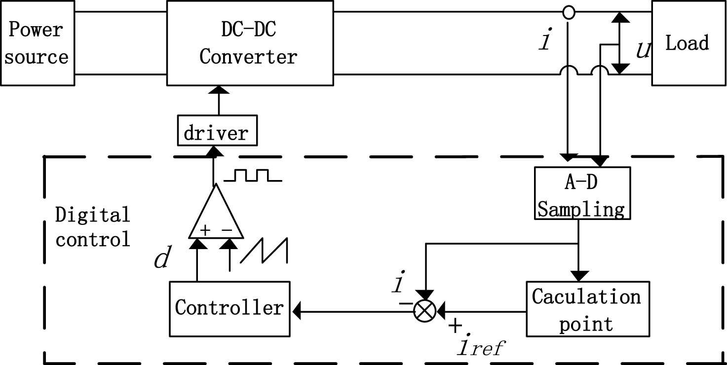
Fig.2
I-V characteristic curves of PV cell.
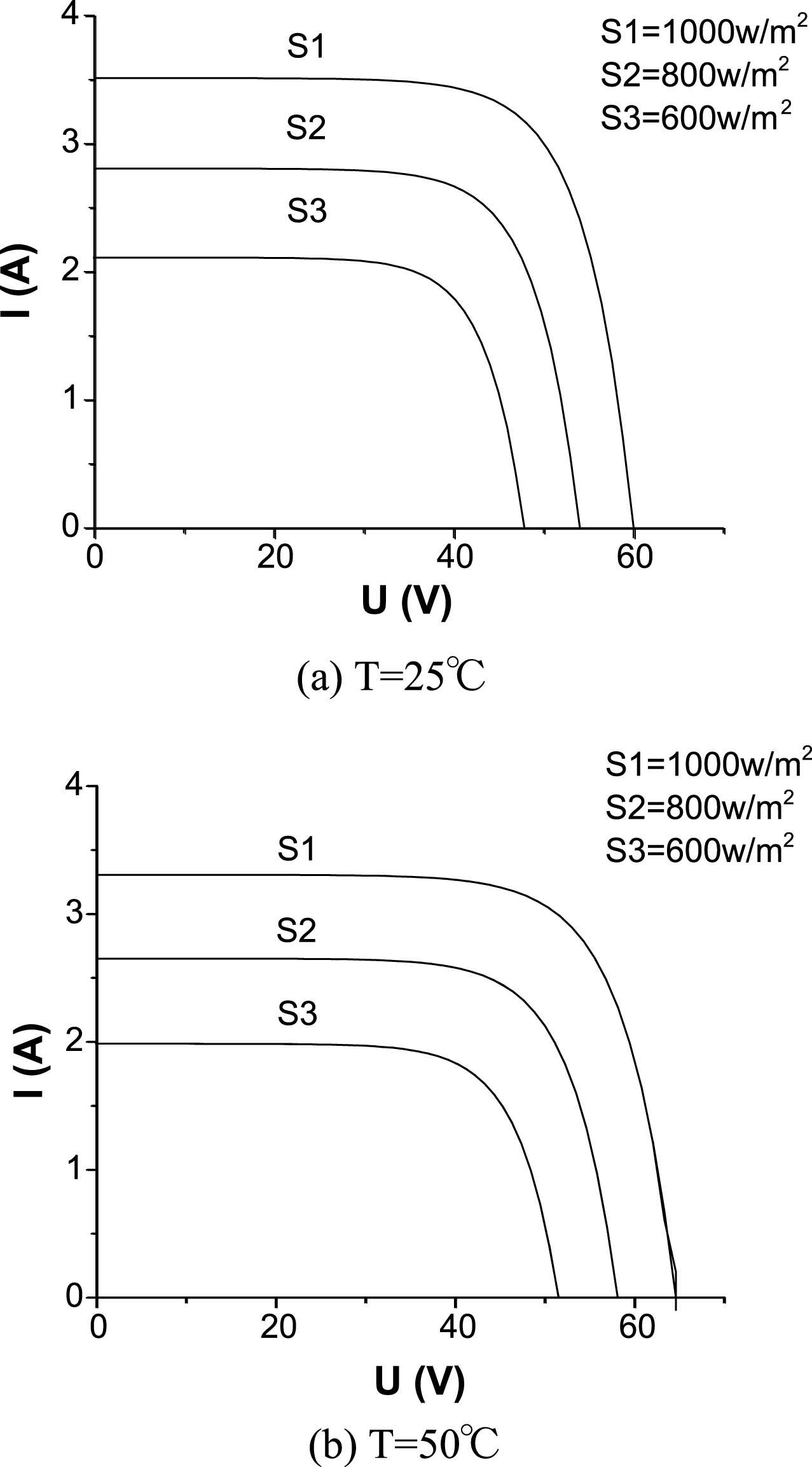
Fig.3
Control objective of simulator.
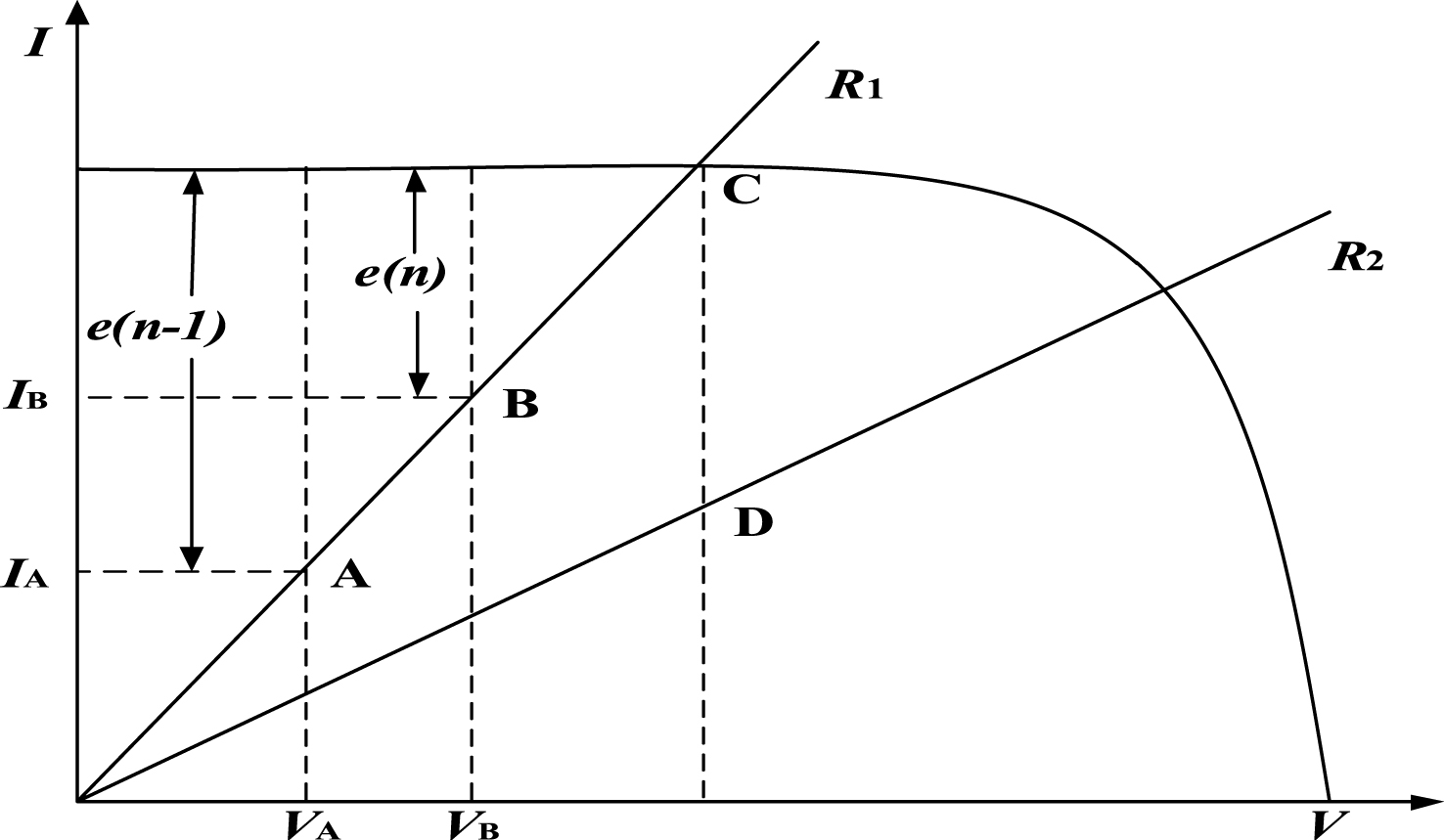
Fig.4
Fuzzy PID controller strategy.
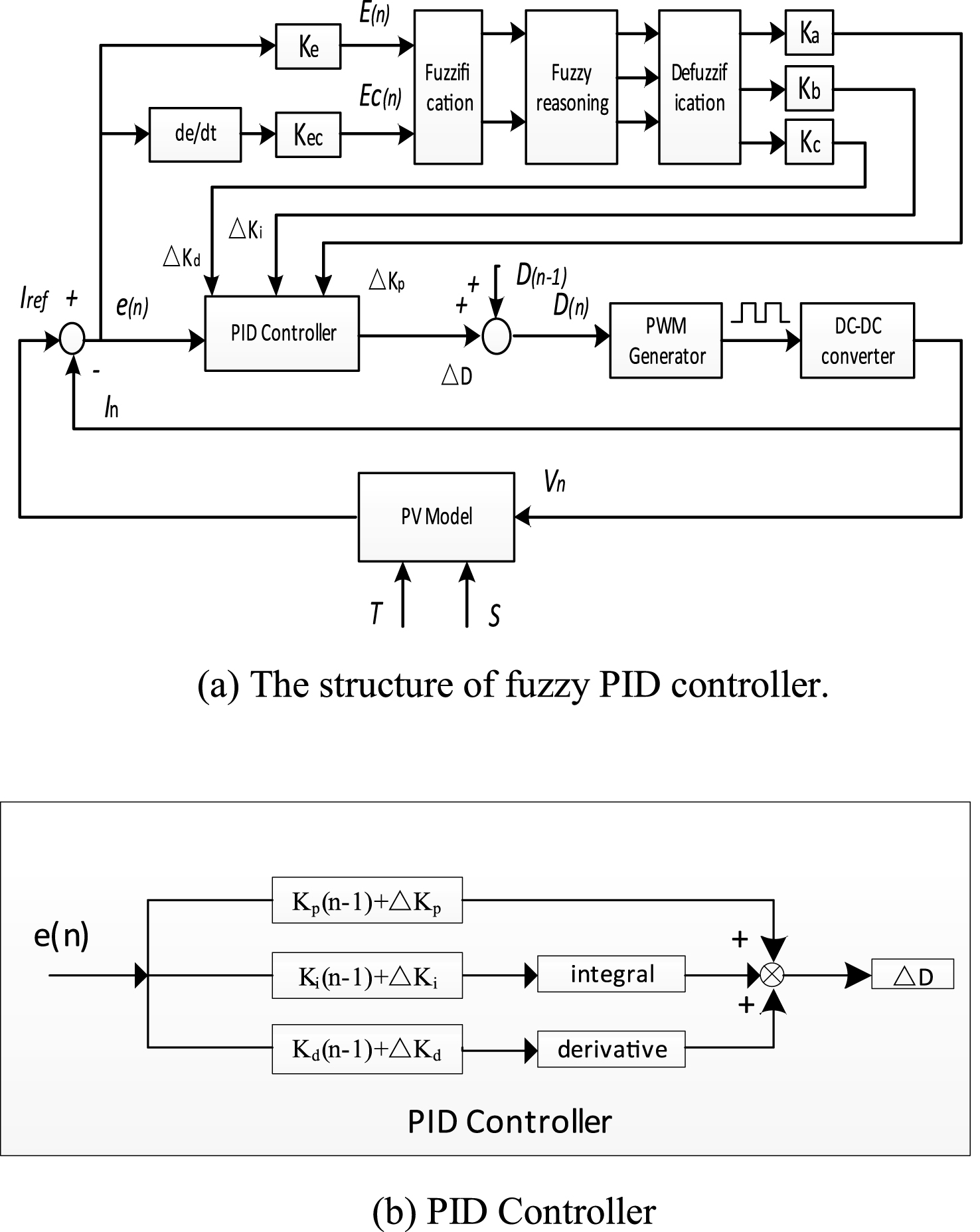
Fig.5
Fuzzy input and output membership functions.
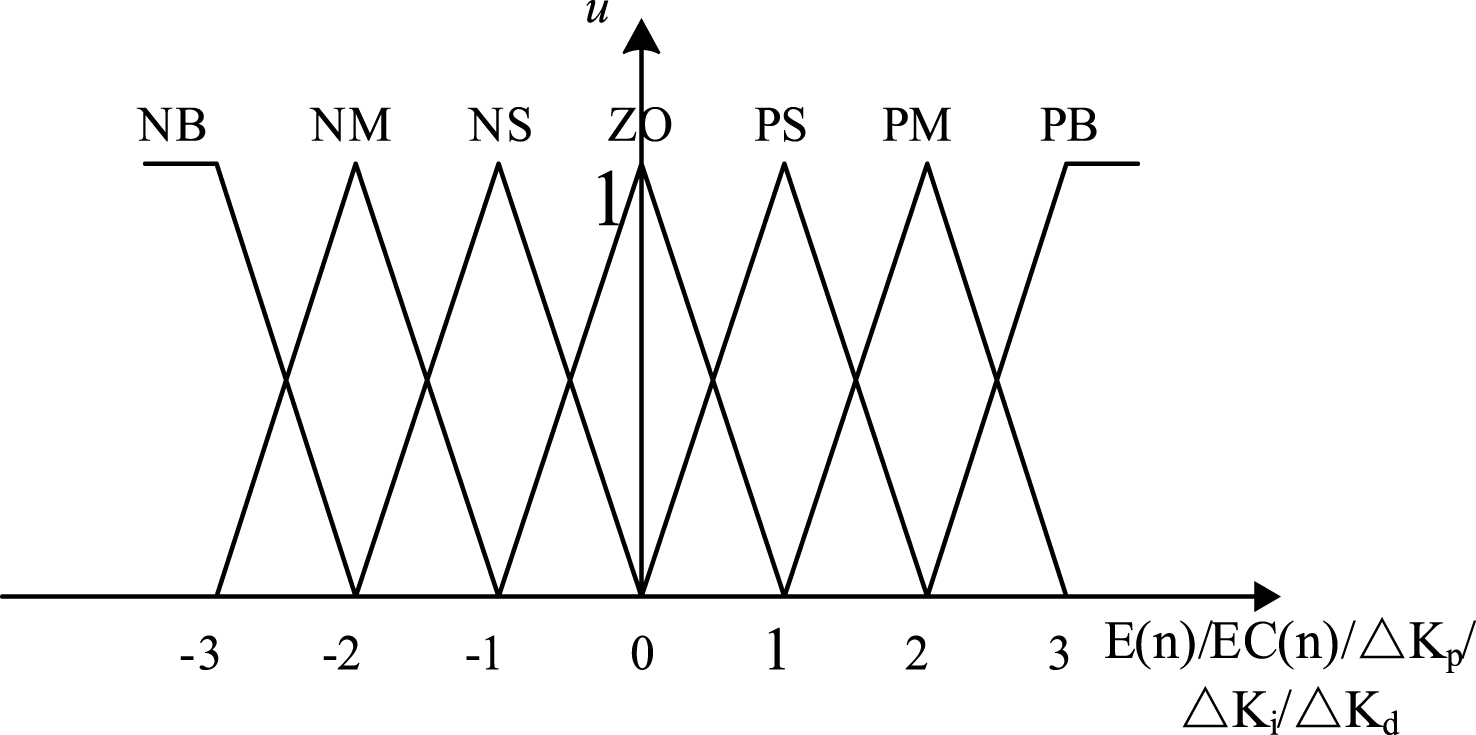
Fig.6
PV cell simulator system.
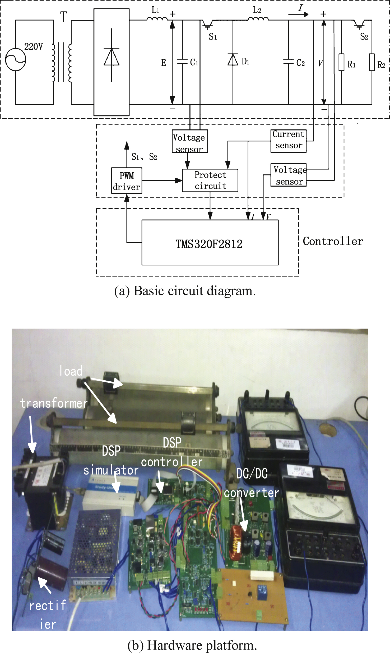
Fig.7
Simulation waveforms of the system startup process and load transformation under different loads.
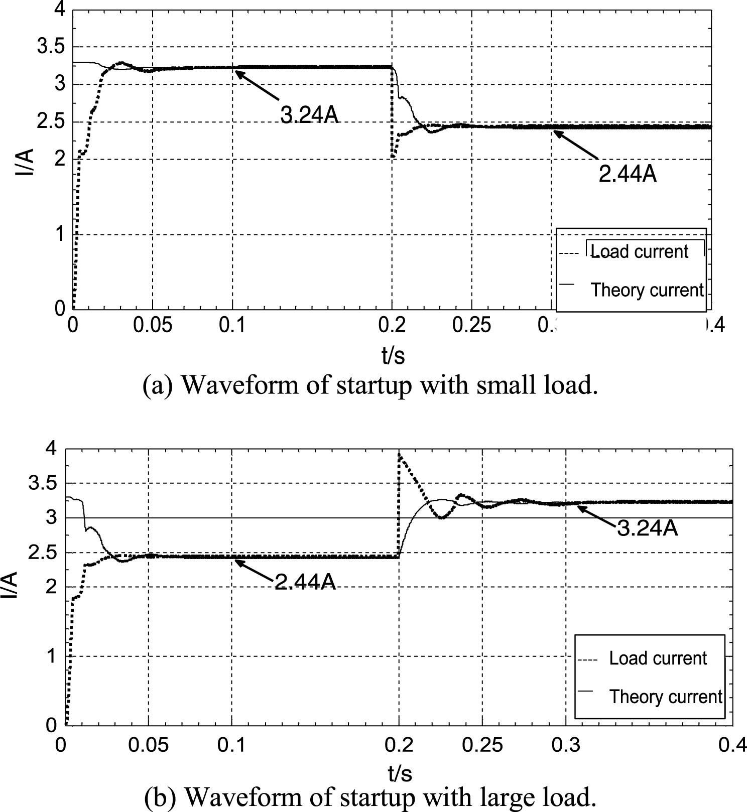
Fig.8
Simulation waveforms of light mutation.
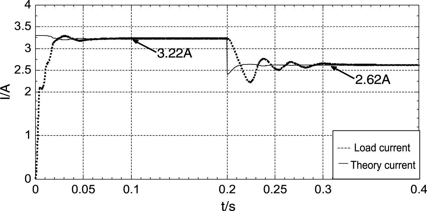
Fig.9
Simulation waveforms of temperature transformation.
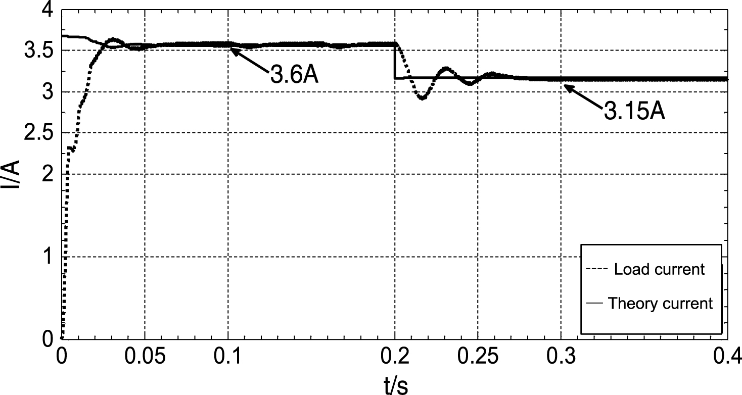
Fig.10
Experimental waveforms of startup performance.
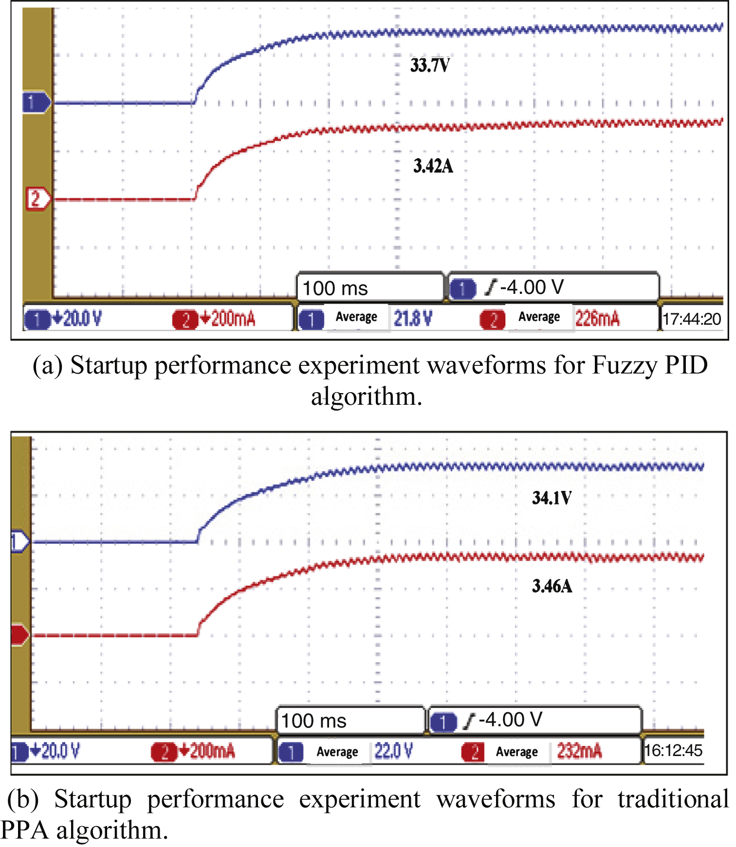
Fig.11
Experimental waveforms of working point mutation based on fuzzy PID algorithm.
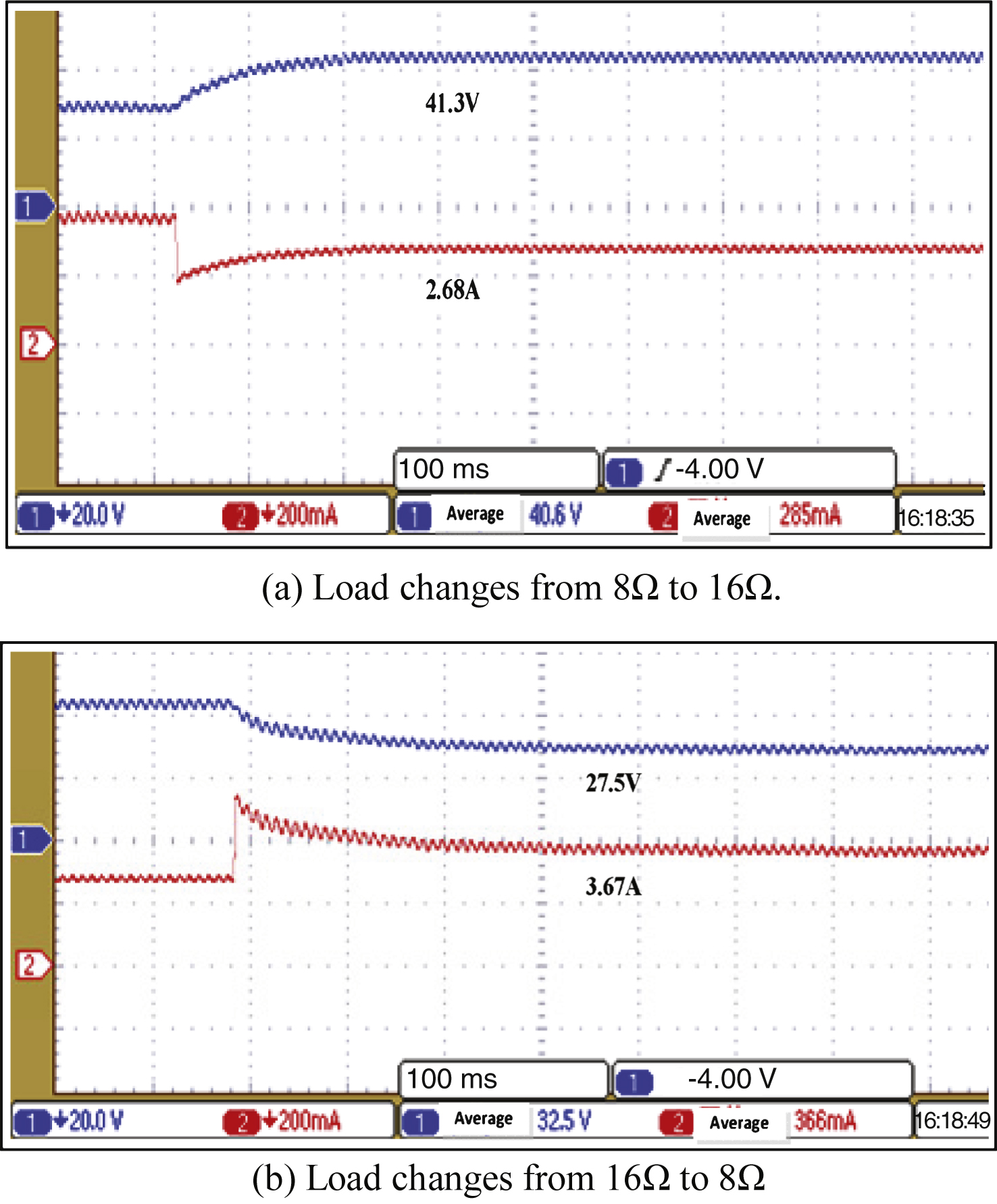
Fig.12
Experimental waveforms of working point mutation based on traditional PPA algorithm.
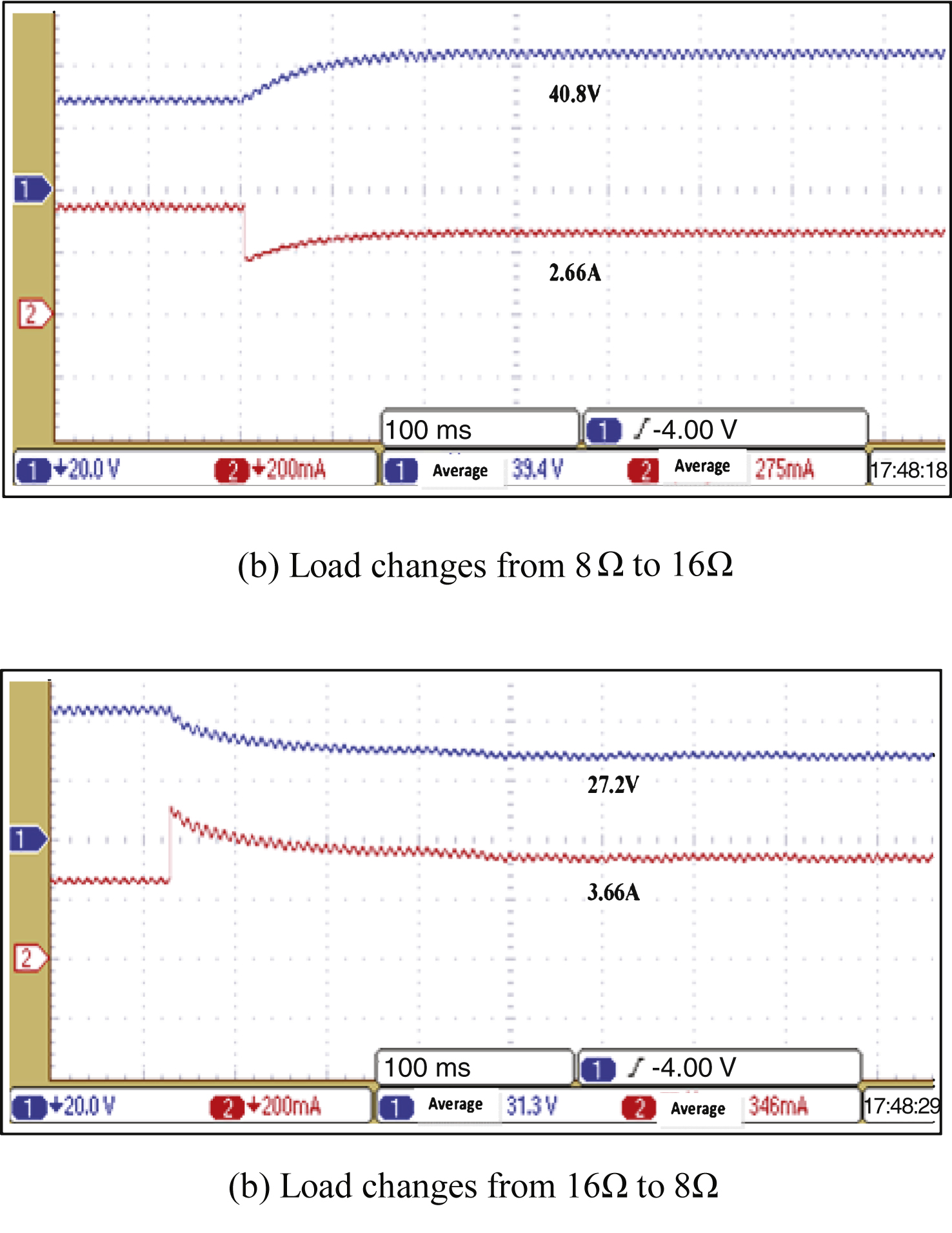
Fig.13
Experimental waveforms of illumination mutation.
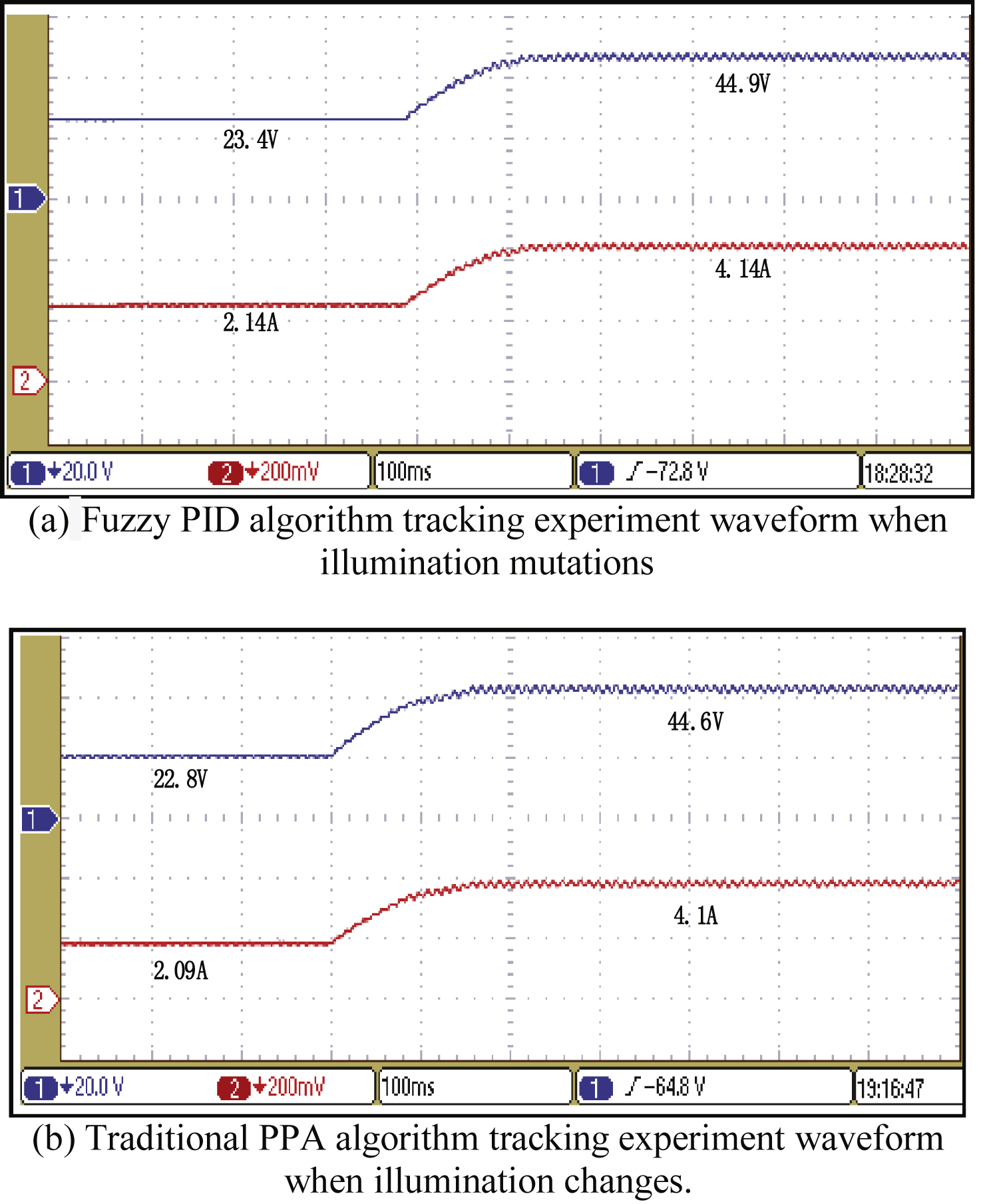
Fig.14
Contrast experiment waveform of temperature change.
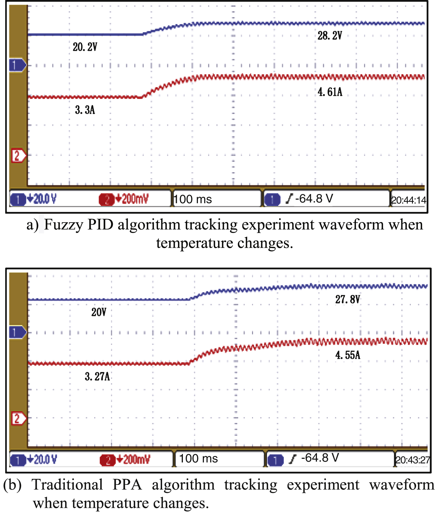
Fig.15
Contrast diagram of I-V simulation curve and experimental point.
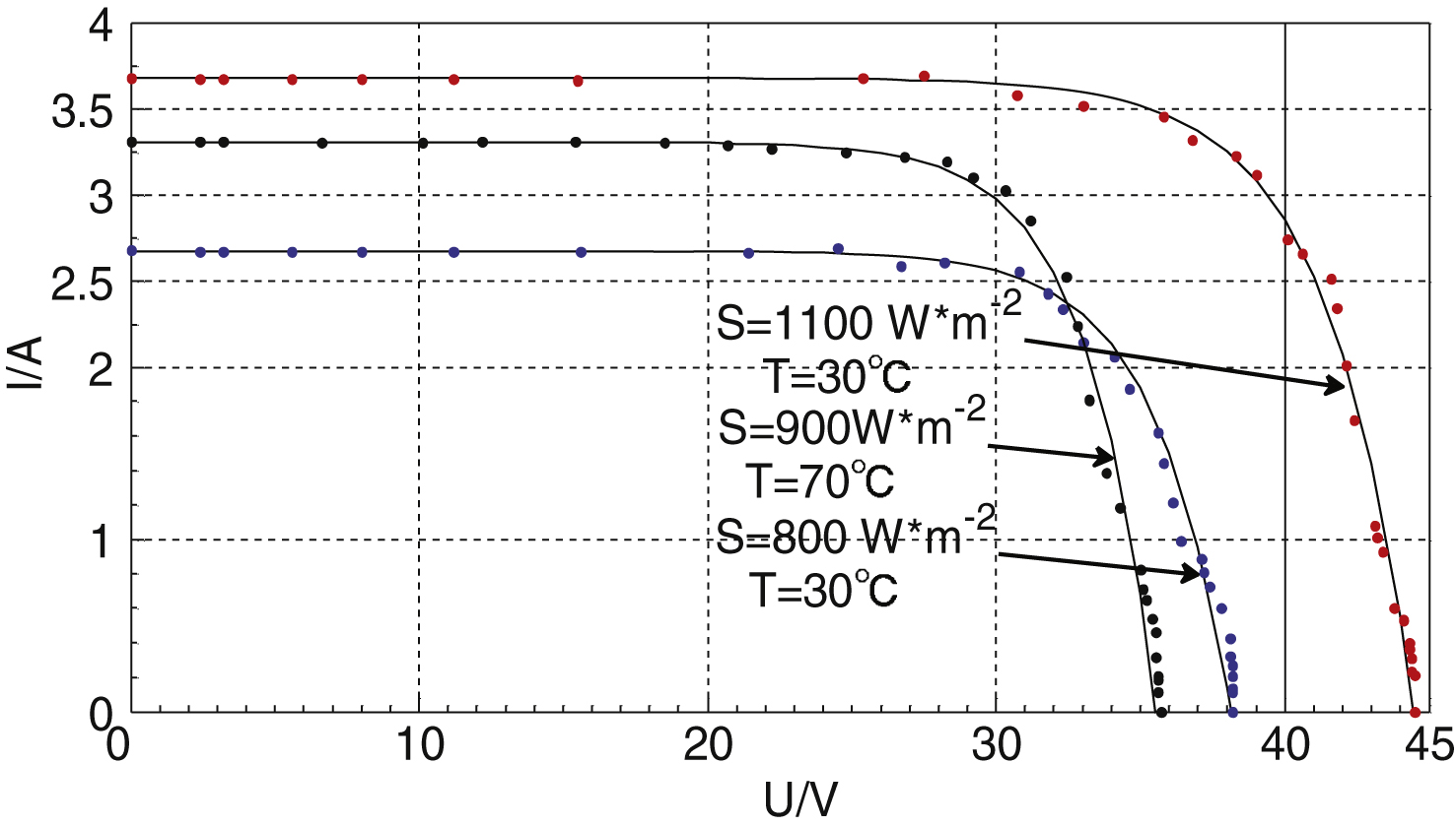
Table 1
Fuzzy control rules of ΔK p
| EC\E | NB | NM | NS | ZO | PS | PM | PB |
| NB | PB | PB | PM | PM | PS | ZO | ZO |
| NM | PB | PN | PM | PS | ZO | ZO | NS |
| NS | PM | PM | PM | PS | ZO | NS | NS |
| ZO | PM | PM | PS | ZO | NS | NM | NM |
| PS | PS | PS | ZO | NS | NM | NM | NM |
| PM | PS | ZO | NS | NM | NM | NM | NB |
| PB | ZO | ZO | NM | NM | NB | NB | NB |
Table 2
Fuzzy control rules of ΔK i
| EC\E | NB | NM | NS | ZO | PS | PM | PB |
| NB | NB | NB | NM | NM | NS | ZO | ZO |
| NM | NB | NB | NM | NS | NS | ZO | ZO |
| NS | NB | NM | NS | NS | ZO | PS | PS |
| ZO | NM | NM | NS | ZO | PS | PM | PM |
| PS | NM | NS | ZO | PS | PS | PM | PB |
| PM | ZO | ZO | PS | PS | PM | PB | PB |
| PB | ZO | ZO | PS | PM | PM | PB | PB |
Table 3
Fuzzy control rules of ΔK d
| EC\E | NB | NM | NS | ZO | PS | PM | PB |
| NB | PS | NS | PB | NB | NB | NM | PS |
| NM | PS | PS | NB | NM | NM | NS | ZO |
| NS | ZO | PS | NM | NM | ZO | NS | ZO |
| ZO | ZO | NS | NS | NS | NS | NS | ZO |
| PS | ZO | ZO | ZO | ZO | ZO | ZO | ZO |
| PM | PN | ZO | PS | PS | PS | PS | PB |
| PB | PB | PM | PM | PM | PS | PS | PB |
Table 4
Parameters of the simulated PV cell
| Open voltage | 43 V |
| Short current | 3.3 A |
| Current (maximum power point) | 3.04A |
| Voltage (maximum power point) | 39.8V |
| Rated power | 110 W |


