Selective and incremental fusion for fuzzy and uncertain data based on probabilistic graphical model
Abstract
Active and dynamic fusion for fuzzy and uncertain data have key challenges such as high complexity and difficult to guarantee accuracy, etc. In order to resolve the challenging issues, in this article a selective and incremental data fusion approach based on probabilistic graphical model is proposed. General Bayesian networks are adopted to represent the relationship among the data and fusion result. It purposively selects the most informative and decision-relevant data for fusion based on Markov Blanket in probabilistic graphical model. Meanwhile we present a special incremental learning method for updating the fusion model to reflect the temporal changes of environment. Theoretical analysis and experimental results all demonstrate the proposed method has higher accuracy and lower time complexity than existing state-of-the-art methods.
1Introduction
Nowadays, wireless sensor networks produce a large amount of data that need to be processed [4], sensor data fusion can be defined as the combination of multiple sensors to obtain more accurate information than using a single sensor. Currently sensor data fusion has been widely used in many application areas including agriculture [16], fault diagnosis [11], geological exploration [20], environmental assessment [1], and etc.
The sensor data fusion algorithms have been developed extensively in past years such as regressionkriging [12], possibility theory [14], evidence theory [7], neural networks [17], diffusion mapping [15], etc.
However, conventional methods always use all the sensors for fusion, but in the real world, since imprecise acquisition devices or the sensor noise, some sensors may produce incorrect, insignificant or irrelevant data for fusion, and using more sensors will also cost more computations, so it is not efficient to use all the sensors for fusion, and purposely choosing an optimal subset (most relevant and informative to decision) from multiple sensing data can save computational time and physical costs, reduce redundancy, and increase the chance of making correct and timely decisions [19]. Furthermore, the conventional methods are static, the fusion models are constant, however, the environments are dynamical and always change over time, sensory observations also evolve over time, so the data fusion system is also needed to reflect temporal changes for dynamic world.
Therefore, a good sensor data fusion system requires the capability which can not only represent the temporal changes of uncertain sensory information, but also purposively select a subset of sensor data those are most decision-relevant for fusion [21], that is active and dynamic data fusion.
To achieve above goals, some tentative researches have been done. Wang, et al. [8] realized active sensor selection based on maximal entropy. Zhang and Ji [21, 22] proposed a tree-like dynamic Bayesiannetwork (DBN) for active and dynamic data fusion, and they applied mutual information to select optimal sensor subset. Liao, et al. [18] proposed to use Influence Diagrams as fusion model, and they proposed an improved greedy approach to select most decision-relevant sensor subset. In addition, they [19] proposed an approximate nonmyopic active sensor selection through partitioning and submodularity based on DBN and greedy algorithm. Kreucher, et al. [3] presented an entropy based active sensing approach, at each time step only one sensor was selected. Guo, et al. [2] proposed an active feature subsets selection method based on mutual information for gait recognition.
But the existing methods face two key challenges, 1) the computation of sensor selection criteria has exponential time complexity; 2) the number of sensor subsets grows exponentially as the total number of sensors [18]. And most methods focus only on sensor selection, can not model the sensor selection, sensor fusion, and decision making in a unified framework. The above challenges lead to high complexity to this problem. Therefore, most researches use approximate method or select only one or few sensors for fusion, so it affects the fusion accuracy in some degree. Though tree-like DBN based methods improve the performance, but they also have four major restrictions. 1) The fusion model is not convenient to be learned from data, so the accuracy of fusion heavily depends on the prior knowledge of experts. 2) Tree-like DBN requires assumption that sensors are independent of each other, but it is not realistic because sensors always have some dependent relationshipsin many applications. 3) The characteristics ofDBN make fusion model difficult to vary with the changing circumstances. 4) It need large amount of DBN inferences which require exponential time complexity.
To address aforementioned problems, in the article, a selective and incremental sensor data fusion approach is proposed. Bayesian network (BN) is adopted to represent relationship of sensor data and fusion result, and it realizes sensor selection and data fusion based on Markov Blanket of BN. It makes the fusion model accommodate the dynamic changes of circumstances through incremental learning from sensor data which generated continuously. The advantages of this method are: it requires no independence assumptions; it requires no BN inference, and it can model the sensor selection, sensor fusion, decision making in a unified framework, so the time complexity is low; the fusion model can reflect the changes of environment better than DBN based methods, so it has high accuracy.
The remainder of this article is organized as follows: Section 2 presented the fusion method we proposed. The experimental results of the proposed method are described in Section 3. Finally, conclusions aresummarized in Section 4.
2Selective and incremental data fusion
In this section, we present the method we proposed, the principles of active fusion based on general BN is presented in Section 2.1, then an algorithm of incremental learning to update the BN dynamically over time is presented in Section 2.2, at last, the overall framework of the method is described in Section 2.3.
2.1Preliminaries of data fusion and BN
In our proposed approach, there are 2 kinds of variables: sensor variable and fusion variable. ‘sensor variables’ represent the information gathered from sensor, and ‘fusion variable’ represent the fusion result, we use S 1, …, S n represent the sensor variables, and F is the fusion variable. The purpose of data fusion is to calculate the value of variable R. A sensor data fusion process can be illustrated as Fig. 1.
A Bayesian network (BN) is a probabilistic graphical model for representing relationships among variables. For a set of variables X = {X 1, X 2, …, X n }, a Bayesian network includes two components:
– A directed acyclic graph in which the node indicates the random variable, and the arc represent relationships of dependency between twovariables;
– For each node X i , it corresponds to a conditional probability distribution P (X i |π i ), where π i indicates the parent set of X i .
The joint probability distribution of X are represented as follows [9, 10]:
For example, Fig. 2(a) is a simple Bayesian network.
2.2Fusion model and sensor selection
In our approach, unlike existing methods, we do not use the tree-like BN, but use general BN to be fusion model, thus the fusion model can obviously present the relationship of sensor data and fusion result. The fusion variable and sensor variables are represented by nodes of BN, if there are n sensor variables, then the BN has n+1 nodes {S 1, …, S n , F}. The result of fusion could be obtained by computing the probability P (F|S 1, …, S n ). For instance, if there are 8 sensors, Fig. 2(b) shows an possible fusion model for our method. It should be pointed out that sometimes one physical sensor may corresponds to multiple sensor variables.
The purpose of selective data fusion is to select a set S * ⊆ {S 1, …, S n }, and the sensor variables of S * are most informative and relevant for fusion. In BN, the Markov Blanket [9] of a node F (denoted as MB(F)) are compose of F’s parent nodes, F’s children nodes and all the parent nodes of F’s children nodes. The Markov Blanket has a property that the MB(F) are the nodes which make F independent of the other nodes of BN [9], viz. P (F|S 1, …, S n ) = P (F|MB (F)), that means given the values of sensor nodes, the probability of F is influenced only by MB (F). So MB (F) is the most relevant and informative sensor data for fusion. Consequently, only the sensor nodes that belong to the MB (F) can be selected for computing the fusion result. In Fig. 2(b), the Markov Blanket of F is {S 2, S 3, S 4, S 5}.
The fusion result can be obtained by computing the P (F|MB (F)). Assuming the range of F is {f 1, …, f k }, so we can select the f i with the highest value of P (F = f i |MB (F)) as the final fusion result. That is:
To calculate the value of above equation, let us consider the following derivation:
Based on the independence assumption of Markov Blanket, we have follow equation based on the characters of Markov Blanket:
Because the denominator P (S 1, …, S n ) does not include F, that means no matter F takes any value, the value of P (S 1, …, S n ) is the same, so it can be viewed as constant. Moreover, the numerator P (R, S 1, …, S n ) is joint probability distribution, so it can be denoted through product of conditional probability distribution of each node. So the above equation can be expressed as follows:
where c is a constant replacing P (S
1, …, S
n
),Children(F) are the children nodes of F. Because
The above equation shows the value of P (F|MB(F)) is proportional to
(1)
Equation (1) contains only the CPT of fusion node F and its children nodes which can be acquired from BN directly, so calculation of fusion result requires no BN inference.
For fuzzy data, for instance, the sensor data is represented as membership function of a fuzzy set. In order to fuse such membership functions, each item (membership degree) of the membership function can correspond to a single node of BN, that is to say one fuzzy sensor data corresponds to multiple sensor variables in BN. Because the value of the item of membership function is real number, we can use the BN with continuous variables to be the fusion model, it is also called continuous BN.
In summary, in this method, the active sensor selection, sensor fusion, decision making are modeled in a unified framework, so it can fuse with high efficiency. The BN model can be established by expert knowledge, machine learning, or the two methods together. The detailed approaches for learning discrete or continuous BN could be looked up in [6, 13].
2.3Incremental updating of fusion model
Sensor data and fusion result generated by one fusion process can compose a new case of sample. After numerous times, the fusion system can gather a group of new data (samples) which can reflect the latest feature of the circumstance. Therefore the BN fusion model can be updated incrementally with novel data. So we present a novel incremental learning algorithm special to update the fusion model. Figure 3 shows an example of incrementally updating process for BN fusion model from time t to t + 1, the structure and parameters of BN all change, and MB (F) also change.
The definition of incremental learning of BN can be described as follows. Supposing that B indicates the current BN, D’ represent the old data gathered before, and D represent the new collected data. In-cremental learning aims to learn new BN B’ which can match the D and D’ well. In the proposed algorithm, we first design a scoring metric that measures the fitness between BN and the data, then proposed a new search strategy to search the best BN which has the highest score.
Based on [5], a modified scoring metric is designed as follows:
In above equation, probability P (D′|B) and P (D|B) evaluates how B fits D’ and the new data. η (0 ≤ η ≤ 1) is learning factor which adjusts the tendency for old or novel data, for instance, if the current fusion model do not match the new data well, i.e. the circumstance has changed substantially, then η would be enlarged to trend the learning procedure to new data. Pen (B) is penalty function to measure the structure of B to make the learning procedure trend to get concise BN which is easy to maintain.
To search the best BN fusion model, we use an improved greedy method. Because the fusion procedure only use the conditional probability distribution of fusion node F and its children, so different from traditional approaches, only local modifications to fusion node and its children nodes can be considered in order to make the search procedure more efficient. The modifications include: reverse an arc, delete or add an arc that ends to F or starts from F; delete or add an arc that ends to F’s child nodes.
| Algorithm 1. Incremental Learning for BN fusion model |
| Input: D; D ′; B |
| Output: B ′; |
| while(not converse) |
| {Score (B) ← η log P (D′|B) + (1 - η) log P (D|B) - pen (B)} |
| Modifications(B)← local modifications to F. |
| |
| B← modify B by m * |
| } |
| return B. |
During the fusion, there are two optional strategies to determine whether to trigger the incremental learning to update model, 1) when the new data fit the fusion model very poorly; 2) when the number of new data reach the specified threshold.
Because we represent the model updating not through transitional probabilities just as in DBN, but based on the data gathered from real environment, and the structure and the parameters of fusion model can all change, so it can reflect the changes of world better than DBN methods.
2.4The overall framework of the proposed method
In a word, the following algorithm summarizes the overall framework of the selective and incremental data fusion procedure based on BN:
| Algorithm 2. Selective and Incremental Data Fusion |
| Input: t; B |
| Output: Result of Fusion FR; |
| /*Select Sensor Variable*/ |
| Discover MB(F) in B; |
| /*Fusion Result Calculation*/ |
| F R
|
| /*Generating new Samples*/ |
| D←D ∪{FR + sensor data}; |
| /*Updating Fusion Model*/ |
| if(t == threshold || the samples fit B badly) |
| B← Incremental Learning (B, D) |
| return FR. |
Above algorithm is only the process of fusion once, so the whole fusion needs to call the algorithm multiple times, in which the parameter t represents the time and is initialized to 0.
In this fusion algorithm, the sensor variables belong to MB(F) in BN are selected firstly, then MB(F) are used to calculate posterior probability of F, at last the value of F which maximizes the posterior probability is selected to be the final fusion result. If the number of new samples reaches the specified threshold or the sample can’t fit the fusion model very well, incremental learning is triggered for updating BN.
3Experiment and result
In this experiment, we use 36 simulated sensors for fusion in the wireless sensor networks. Due to space limitation, the fusion model structure is not listed in this paper. Every time when the fusion system collects 200 cases of new data, incremental learning is triggered for updating the fusion model, then we validate accuracy of fusion, with the purpose of making the test results more precise, we use 1000 samples to test the average percent of accuracy by comparing the fusion result generated by the fusion model with the real fusion result in the sample. Thereby we compare the proposed method with other state-of-the-art methods in both accuracy and running time.
Figure 4 demonstrate the accuracy of our approach and the state-of-the-art methods, where “DBN method” represents the methods based on DBN and “Passive method” represents passive fusion method (randomly select sensors). We can observe that because our method and DBN method are active fusion, so they have much higher accuracy than passive fusion. And in the beginning, the accuracy of the proposed method is similar to DBN method, however, just as we discussed in Section 2, the proposed method can vary with the changing environment better, so it shows higher accuracy than DBN method as time goes on.
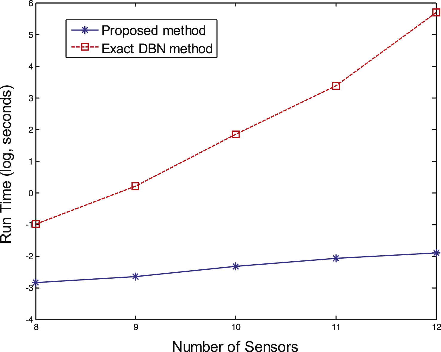
Figure 5 illustrates average computational time with the proposed method versus fusion method based on exact optimal search and DBN inference. The comparison is made in various numbers of sensors. We can observe that when the number of sensors is small, the run time is similar. But with the number growing, the computational time of exact method exponentially increases, and the run time of the proposed method increases almost linearly. Therefore, the proposedmethod can save more time.
We also made an experiment about real sensor data which is to fuse the temperature, humidity and PM2.5 sensor data to evaluate whether the environment is comfortable to human. And the results are also accurate to verify the validity of the approach.
4Conclusions and future works
To achieve rapid and precise sensor data fusion, in this article a selective and incremental data fusion approach based on graphical probabilistic models was proposed. This method models the sensor selection, sensor fusion, decision making in a unified framework, it uses the general BN to indicate the relationship among fusion result and sensor data. The active sensor selection can be performed by discovering Markov Blanket of fusion variable. The fusion model is updated through incremental learning of BN. Theoretical analysis and experimental results both show the proposed method has higher accuracy and lower time complexity than existing methods. In future, we will do more experiments to compare the proposed method to other traditional and the latest methods, and apply the proposed method to more real scenarios.
Acknowledgments
This research is supported by the NSFC (61133011, 61502198, 61373053, 61472161 and 61202308), China Postdoctoral Science Foundation (2013M541303), the Opening Fund of State Key Laboratory of Applied Optics, Science and Technology Development Programof Jilin Province of China (20150520066JH and 20130206046GX).
References
1 | Smeaton AF, O’Connor E, Regan F (2014) Multimedia information retrieval and environmental monitoring: Shared perspectives on data fusion Ecological Informatics 23: 118 125 |
2 | Guo B, Nixon MS (2009) Gait feature subset selection by mutual information IEEE Transactions on Systems, Man, and Cybernetics-Part A: Systems and Humans 39: 1 36 46 |
3 | Kreucher C, Kastella K, Hero AO (2005) Sensor management using an active sensing approach Signal Process 85: 3 607 624 |
4 | Nakamura EF, Loureiro AAF, Frery AC (2007) Information fusion for wireless sensor networks: Methods, models, and classifications ACM Computing Surveys 39: 3 1 55 |
5 | Wang F, Liu DY, Wang SX (2005) Research on incremental learning of Bayesian network structure based on genetic algorithms Journal of Computer Research and Development 42: 9 1461 1466 |
6 | Elidan G, Nachman I, Nachman F (2007) Ideal parent structure learning for continuous variable Bayesian networks Journal of Machine Learning Research 8: 1799 1833 |
7 | Lin GP, Liang JY, Qian YH (2015) An informationfusion approach by combining multigranulation rough sets and evidence theory Information Sciences 314: 184 199 |
8 | Wang H, Yao K, Pottie G, Estrin D (2004) Entropy-based sensor selection heuristic for target localization 3rd International Symposium on Information Processing in Sensor Networks 36 45 Berkeley, USA |
9 | Pearl J (1988) Probabilistic Reasoning in Intelligent Systems Morgan Kaufmann Burlington, USA |
10 | Campos LM (2006) A scoring function for learning Bayesian networks based on mutual information and conditional independence tests Journal of Machine Learning Research 7: 2149 2187 |
11 | Safizadeh MS, Latifi SK (2014) I Using multi-sensor data fusion for vibration fault diagnosis of rolling element bearings by accelerometer and load cell Information Fusion 18: 1 8 |
12 | Meng QM, Borders B, Madden M (2010) High-resolution satellite image fusion using regression kriging International Journal of Remote Sensing 31: 7 1857 1876 |
13 | Daly R, Shen Q, Aitken S (2011) Learning Bayesian networks: Approaches and issues The Knowledge Engineering Review 26: 99 157 |
14 | Destercke S, Dubois D, Chojnacki E (2009) Possibilistic information fusion using maximal coherent subsets IEEE Transactions on Fuzzy Systems 17: 1 79 92 |
15 | Lafon S, Keller Y, Coifman RR (2006) Data fusion and multicue data matching by diffusion maps IEEE Transactions on Pattern Analysis and Machine Intelligence 28: 11 1784 1797 |
16 | Mahmood Hafiz S, Hoogmoed Willem B, van Henten Eldert J (2012) Sensor data fusion to predict multiple soil properties Precision Agriculture 13: 6 628 645 |
17 | Sajjad S, Faridoon S, Dan S (2014) Multirate multisensor data fusion for linear systems using Kalman filters and a neural network Aerospace Science and Technology 39: 465 471 |
18 | Liao WH, Ji Q (2006) Efficient active fusion for decision-making via VOI approximation 21st AAAI Conference on Artificial Intelligence (AAAI-2006) 1180 1185 Boston, USA |
19 | Liao WH, Ji Q, Wallace WA (2009) Approximate nonmyopic sensor selection via submodularity and partitioning IEEE Transactions on Systems, Man, and Cybernetics-Part A:Systems and Humans 39: 4 782 794 |
20 | Shi WZ, Tian Y, Huang Y, Mao HX, Liu KF (2009) A two- dimensional empirical mode decomposition method with application for fusing panchromatic and multispectral satellite images International Journal of Remote Sensing 30: 10 2637 2652 |
21 | Zhang YM, Ji Q (2006) Active and dynamic information fusion for multisensor systems with dynamic Bayesian networks IEEE Transactions on Systems Man and Cybernetics-Part B: Cybernetics 36: 2 467 472 |
22 | Zhang YM, Ji Q (2010) Efficient sensor selection for active information fusion IEEE Transactions on Systems, Man, and Cybernetics- Part B: Cybernetics 40: 3 719 728 |
Figures and Tables
Fig.1
Overview of sensor data fusion process.
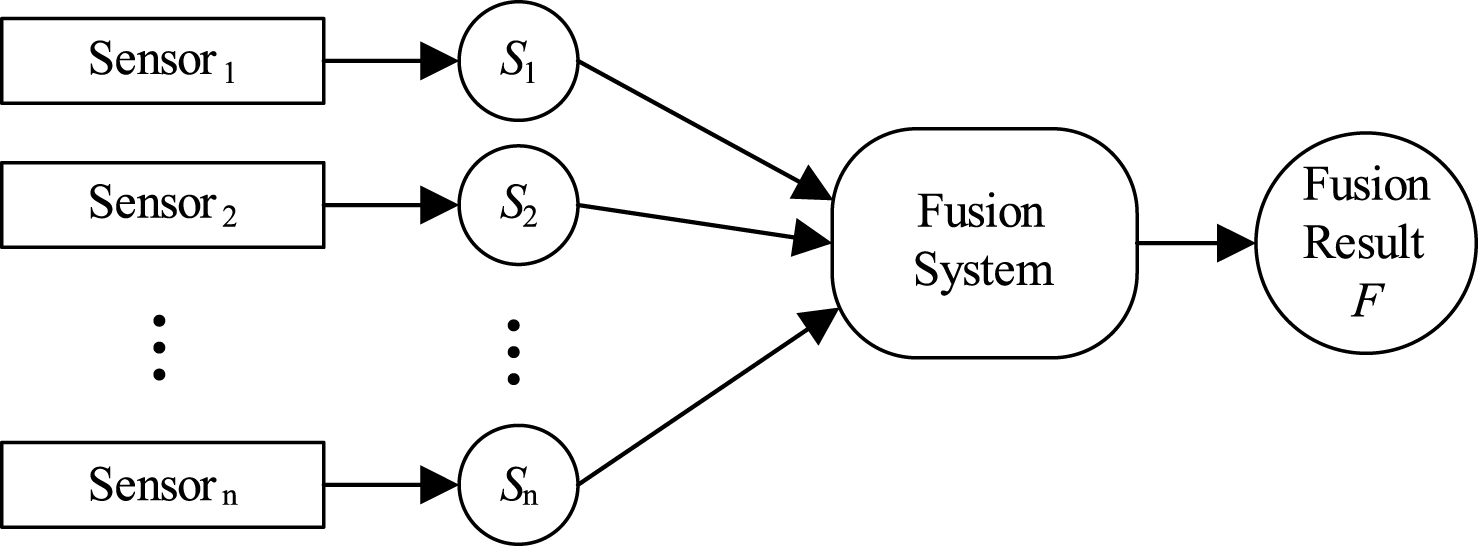
Fig.2
(a) An instance of BN with 9 variables. (b) An instance of BN for sensor data fusion in proposed approach.
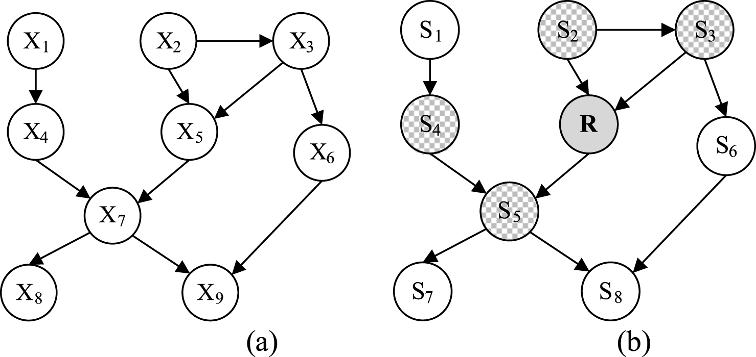
Fig.3
An instance of incrementally updating BN.
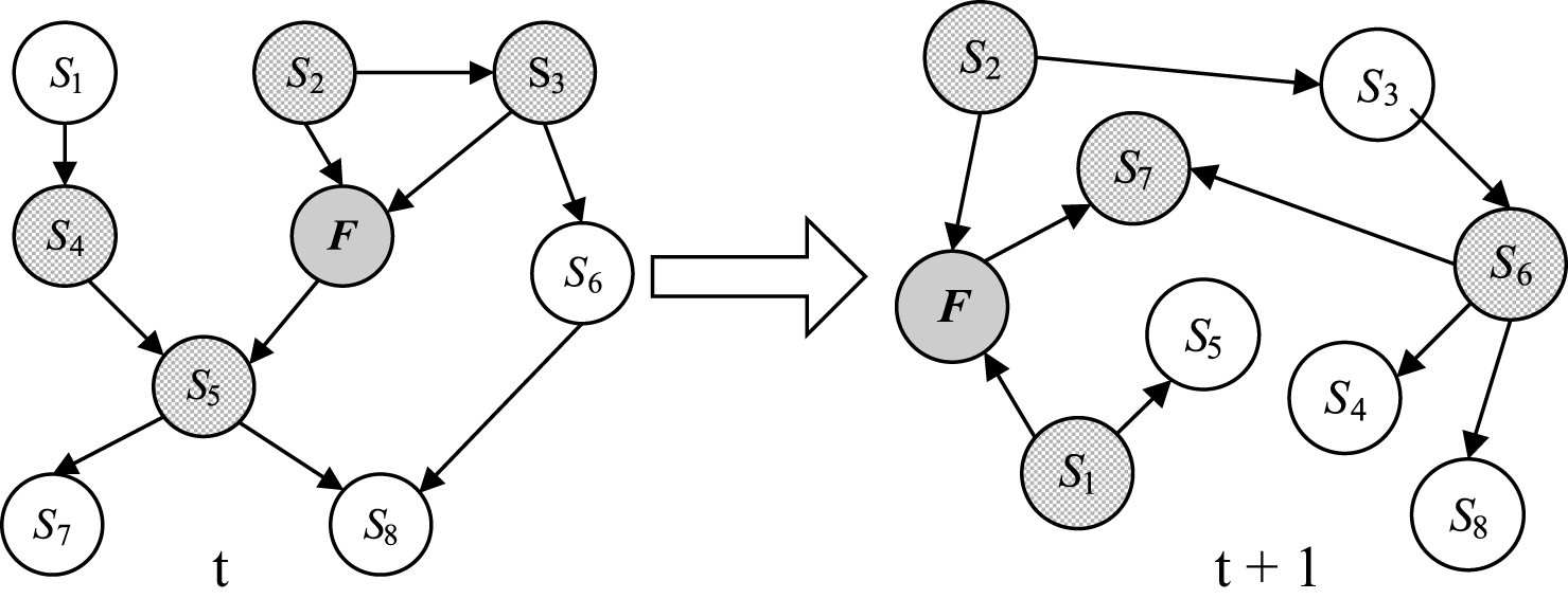
Fig.4
Comparison of accuracy of the three approaches.
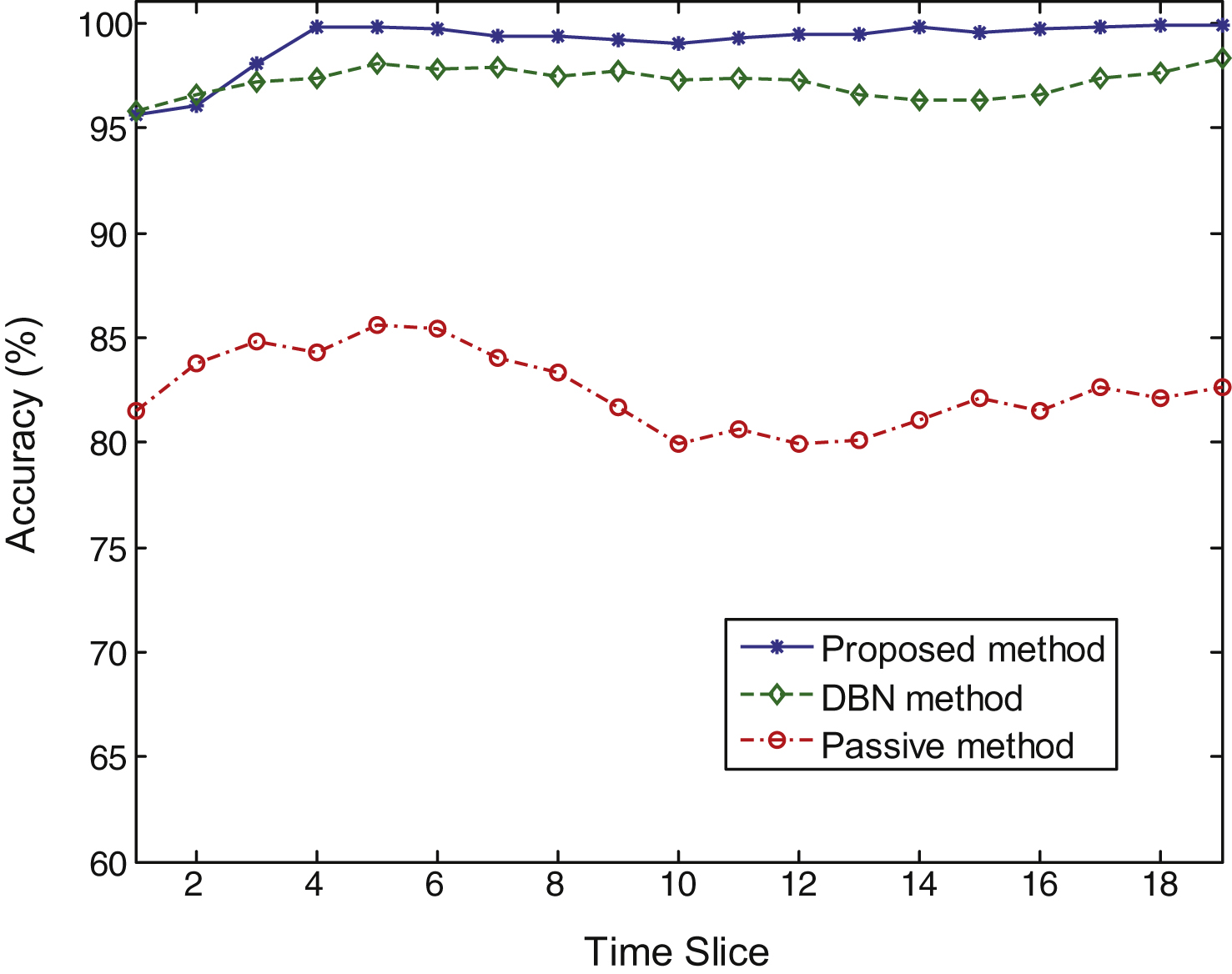
Fig.5
Average running time of the proposed method and exact DBN based method with various numbers of sensors.