
Rule-based fuzzy classifier based on quantum ant optimization algorithm
Abstract
Fuzzy rule-based classification systems have been used extensively in data mining. This paper proposes a fuzzy rule-based classification algorithm based on a quantum ant optimization algorithm. A method of generating the hierarchical rules with different granularity hybridization is used to generate the initial rule set. This method can obtain an original rule set with a smaller number of rules. The modified quantum ant optimization algorithm is used to generate the optimal individual. Compared to other similar algorithms, the algorithm proposed in this paper demonstrates higher classification accuracy and a higher convergence rate. The algorithm is proved to be convergent on theory. Some experiments have been conducted on the algorithm, and the results proved that the algorithm is feasible.
1Introduction
During the past several decades, there has been much reported research on fuzzy control systems to control widely diverse systems, such as car automation systems, classification systems of data mining, cart centering problems, truck backing problems, etc. Previous research particularly focuses on the application of fuzzy systems to these various control problems; fuzzy if-then rules are typically employed, and are usually derived from human experts. Recent research has addressed the automatic generation of fuzzy if-then rules from measured data in real-world situations, without human experts. These self-learning methods have been proposed for adjusting membership functions of fuzzy sets in fuzzy rules, using methods such as gradient descent, neural networks, and genetic algorithms.
The fuzzy rule-based classification system (FRBCS) is considered to be a very useful tool in computational intelligence, since it provides a very interpretable model for end users. The FRBCSs consist of two main components: the Inference System and the Knowledge Base (KB). The KB is composed of the Rule Base (RB) constituted by the collection of fuzzy rules, and the Data Base (DB), which contains the membership functions of the fuzzy partitions associated with the linguistic variables. The composition of the KB depends directly on the problem to be solved. If there is no expert information regarding the problem to be solved, an automatic learning process must be employed to derive the KB from examples.
Genetic algorithms have been widely proposed to generate fuzzy if-then rules and tune the membership function of fuzzy sets in fuzzy rules [1–10]. J.R. Kim and D.U. Jeong proposed a genetic algorithm-based approach to a fuzzy rule-based system for fuzzy classification with a minimum of fuzzy rules [3]. Z.Y. Xing, Y.L. Hou, et al. proposed a novel method based on a multi-objective genetic algorithm to construct a fuzzy classification system [10].
This paper proposes a fuzzy rule-based classification algorithm based on quantum ant optimization algorithm is proposed (FRBCA-QANO). The method of generating the hierarchical rules with various granularity hybridizations is used to generate the initial rule set. The modified quantum ant optimization is used to solve the problem of rule selection. The algorithm is proved to be convergent on theory, and experimental result confirms that the algorithm is convergent and feasible.
2Algorithm model
2.1Fussy classification
Considering an object which can be described as a point in a characteristic space (x ∈ S N ), the classification assigns the point a class out of M possible classes {C 1, C 2, …, C M }. The key problem of the classification is to find an optimal map D : S N → C.
The fuzzy rules are used to describe the knowledge in the fuzzy classification system, and fuzzy inference methods are used to construct a knowledge base. The fuzzy rule set is included in the rule base. The antecedents of the fuzzy rules define local fuzzy regions, while the consequents describe the classification labels within those regions. Supposed that there is a data set with k samples, T = {(x
1, c
1) , …, (x
k
, c
k
)}, where
Ri: IF X 1 is A li AND … XN is ANi then Y is Ci with ri, where ri represents the accuracy of an example which belongs to to class ci; and Aji is the membership function defined on the domain of the attribute, which can be triangular, Gaussian-shaped, a trapezoidal function, etc. The support and confidence of the association rules are used to choose the rules. The fuzzy rule is considered to be the associate rule, which is described as follows.
(1)
where A q is the antecedent of the rule, and C q is the consequent of the rule. These two conceptions are extended to the fuzzy association rule. The extended forms proposed by Isibuchi and Yamamoto are used in this paper.
The confidence of A q ⇒ C q can be defined asfollows.
(2)
where D is a training set with m samples;
(3)
where μ A q (x p ) can be a product or minimum; theproduct is used in this paper.
(4)
where
The support degree of the rule A q ⇒ C q can be described as follows.
(5)
where |D| represents the number of samples in thetraining set. In the same way, the support degree can be redefined as follows.
(6)
The antecedent is the fuzzy rule of A q , therefore the consequence C q can be calculated as follows.
(7)
The consequence of the rule is the class which has the maximum confidence degree out of M classes. When the support degree is used instead of the confidence degree, the result identical, because they demonstrate the following relationship.
(8)
2.2Encoding method
A quantum bit as an information storage unit represents a two-state quantum system. It is a unit vector defined in a two-dimensional complex vector space. The space is composed of standard orthogonal basis {|0〉 , |1 〉 }. Therefore, it can be in the quantum superposition simultaneously. The state can be represented as follows [13, 14].
(9)
where α and β are complex numbers that specify the probability amplitudes of the corresponding states. |α|2 is the probability that the Q-bit will be found in the “0” state and |β|2 is the probability that the Q-bit will be found in the “1” state. Normalization of the state to unity guarantees Equation (10).
(10)
If there is a system of m Q-bits, the system can simultaneously represent 2m states. However, in the act of observing a quantum state, it collapses into a single state.
In this paper, there are two parts in the chromosome (C = C1+C2). There are m bits in the C1, and if the bit is 1, the corresponding rule is selected; otherwise is the rule is not used. There are m real numbers in the C2 portion; the real number represents the weight of the related rule. The real number in the interval [0, 1] can be directly encoded with the quantum bit of probability amplitude. The encoding can be described as follows.
(11)
The position of an ant represents a solution of the problem in the continuous ant colony optimization algorithm. Suppose that there are n ants, which are distributed randomly in the 2 m-dimensional space [–1, 1]T. Each ant has 2 m quantum bits, and the probability amplitude represents the current position of the ant.
Fuzzy modeling requires the consideration of multiple objectives in the design process, including classification performance and interpretability. In this paper, classification performance is defined as the number of training patterns, which are classified correctly and denoted as f1. Interpretability is the number of fuzzy rules, denoted as f2. The object function is described as follows.
(12)
where ω 1 and ω 2 are the weighs of f 1 and f 2, respectively.
2.3Select ants moving to target location
Set τ (x r ) as the pheromone intensity of the k ant, which is at the position of x k . It is initialized as a constant. Set η (x r ) as the visibility of the position of x k . The probability of the ant k moving from x r to x s is described as follows.
(13)
2.4Quantum rotation gate
The rotation operation updates the quantum bit (Q-bit) by using rotational gate. This operation makes the ant population develop into the best individual. The Q-gate is defined by Equation (14).
(14)
The Q-bit is updated as follows.
(15)
Equation (15) indicates that this updated operation only changes the phase of the Q-bit, but does not alter the length of the Q-bit.
where Δθ is the rotation angle of each Q-bit. The magnitude of Δθ has an effect on the speed of convergence; if it is too large, the solution may diverge or converge prematurely to a local optimum. The sign of Δθ determines the direction of convergence, and Δθ can be determined according to the following method. α 0 β 0 is the probability amplitude of the global optimal solution in the current search, and α 1 β 1 is the probability amplitude of the Q-bit in the current solution. Define A as follows.
(16)
The direction of Δθ can be determined as follows. If A ≠ 0, the direction is -sgn(A); if A = 0, the direction can be selected randomly.
In order to avoid premature convergence, the size of Δθ can be determined according to Equation (10), as described. This method is a dynamic adjustment strategy and is unrelated to the problem; pi is the circumferential ratio, and maxGen represents the maximal number of iterations.
(17)
2.5Update rules of pheromone intensity and visibility
The function of the optimal problem is responsible for evaluating the ant position, and the primary goal of pheromone intensity updating is to integrate function value with the pheromone. Better function values result in higher pheromone intensities. The gradient information of the function is also integrated with the visibility, indicating that a position with greater gradient also has greater visibility. The point determined according to this method not only has higher fitness, but also a higher rate of change.
Each ant computes the function value after one step research, and updates the local pheromone intensity and the visibility according to the rules given as follows. Suppose that the previous position of the ant is x q , the current position is x r , and the next position is x s . The updating rule is described as follows.
(18)
(19)
(20)
(21)
If the function f is a non-differentiable function, the first difference can be used. It is described as follow.
(22)
where 0 < α < 1, 0 < β < 1. After all ants have completed a cycle, the global pheromone intensity is updated according to Equation (23). The (1 - ρ) is the volatility coefficient of the pheromone where 0 < ρ < 1, and
(23)
3Convergence analysis
Theorem 1: The FRBCA-QANO algorithm ant population sequence {Q (t) , t> 0 } is the finite homogeneous Markov chain.
Proof: The Q-bits are used in the algorithm. In the ant colony evolution algorithm, the value of the ants is discrete. Assume that the length of the ant is 2 m and the ant population size is n, therefore the state space size is 2mn. Due to the continuity of the variable value, the size of the state space size is infinite in theory, but the accuracy is finite during calculation. Assuming that the dimension is V, then the state size of the population is V 2mn, and so the population is finite. In the algorithm, the rotational operation is entirely independent of the generation number, the pheromone intensity is updated according to Equation (18), and the visibility is updated according to Equation (20). All of these are independent of the generation number. Therefore the population sequence is a finite homogeneous Markov chain.
Definition 2. f k = max {f (x i ) , i = 1, 2, …, N} is a random variant sequence. The variable represents the best solution in the k generation. If the condition satisfies Equation (24), then the algorithm is convergent to the global optimal solution with a probability of 1.
(24)
Theorem 2. The FRBCA-QANO algorithm is convergent to the global optimal solution with a probabilityof 1.
Proof. According to Theorem 1, the ant is a finite homogeneous Markov chain. Suppose that the ant population is 2 m, and the ants are points in the research space Ω. X
i
∈ Ω indicates that X
i
is a point in Ω. X
i
={ x
1, x
2, …, x
n
},
During the transfer procedure, there are two special situations.
– The first situation is that
– The second special situation is when
The proof of convergence is described below, noting that it does not apply to the two above-mentioned special situations. Suppose that X
k
is at position s
i
, and the possibility is
(25)
(26)
(27)
According to Equations (27, 28) is obtained.
(28)
Equation (28) is substituted into Equations (21), and (29) is obtained.
(29)
According to the two special situation described above,
4Simulation experiment
The Iris system is a common benchmark problem in classification and pattern recognition studies. It contains 150 measurements of four features (sepal length, sepal width, petal length, petal width) from each of three species (Setosa, Versicolor, Virginica). Therefore, there are four independent variables that form the antecedent of the rule, and three dependent variables that form the consequence of the rule. From each species, there are 50 observations regarding sepal length, sepal width, petal length and petal width (in cm).
In the simulation experiment, the variables are set as follows. The ant populate size m is 50, the size of quantum n = 8, volatility coefficient (1 - ρ) = 0.3, the pheromone update exponent α= 0.5, the visibility exponent β= 0.5, the corner step θ 0 = 0.05*pi, and ω 1 = 1, ω 2 = 0.1. In order to avoid influence of change in the experiment, all programs were run 20 times. The final fuzzy classification system is described as follows.
R1: if x3 is A31, x4 is A41, then x belongs to Class 1, CF = 0.21.
R2: if x3 is A32, x4 is A42, then x belongs to Class 2, CF = 0.42.
R3: if x3 is A33, x4 is A43, then x belongs to Class 3, CF = 0.38.
To prove the validity of QACO, it is compared to the conventional classification algorithm; results are shown in Table 1. As shown in Table 1, the three algorithms can obtain the same rule number, but the FRBCA-QANO demonstrates higher accuracy and less variability.
In order to prove the efficiency of the algorithm, it is compared to a fuzzy classifier based on the Mamdani fuzzy logic system and the genetic algorithm (FCMFLSGA) [9]. The standard genetic algorithm is used in the algorithm FCMFLSGA. In the FCMFLSGA experiment, the population size is 100, and cross-probability Pc is 0.9. The mutation probability Pm is 0.1. Experimental results are described in Figs. 1 and 2.Figure 1 indicates that the FRBCA-QANO demonstrates a higher convergence rate and accuracy than FCMFLSGA. According to Fig. 2, a conclusion can be drawn that the algorithm FRBCA-QANO also demonstrates a higher convergence rate than algorithm FCMFLSGA.
5Conclusion
A fuzzy rule-based classification algorithm based on the quantum ant optimization algorithm is proposed. The method of generating the hierarchical rules with various granularity hybridizations is used to generate the initial rule set. This method can obtain an original rule set with fewer rules, and enhance the convergence rate of the algorithm. The modified quantum ant colony optimization (MQACO) is used to solve the problem of rule selection from the original rule set. The MQACO ensure that the algorithm has a higher classification accuracy and higher convergence rate than similar algorithms. The algorithm is proved to be convergent on theory, and experimental results also confirm that the algorithm is convergent and feasible.
Acknowledgments
This research was supported by the National Key Basic Research and Development Program (2014CB744100), the foundation of continuing education of Southwest University of Science (13JYF01), the doctoral fund of the Southwest University of Science (13ZX7102) and the research project of Sichuan Education Bureau (12ZB328, 12ZB327).
References
1 | Lim CG, Jung YM, Kim EK (2003) A genetic algorithm for generating optimal fuzzy rules International Journal of KIMICS 7: 765 778 |
2 | Pooya H, Taghi ASM (2013) Online adaptive fuzzy logic controller using genetic algorithm and neural network for networked control systems The Proceedings of 15th International Conference on Advanced Communications Technology (ICACT) 88 98 PyeongChang, Korea |
3 | Kim JR, Jeong DU (2008) Optimizing the fuzzy classification system through genetic algorithm The Proceedings of the Third International Conference on Convergence and Hybrid Information Technology 903 908 Busan, South Korea |
4 | Ray MI, Galende M, Sainz GI, Fuente MJ (2013) Selection of rules by orthogonal transformation and genetic algorithm to improve the interpretability in fuzzy rule based systems The Proceedings of IEEE International Conference on Fuzzy Systems (FUZZ) 1 8 Hyderabad, India |
5 | Villar P, Fernandez A, Herrera F (2011) Studying the behavior of a multiobjective genetic algorithm to design fuzzy rule-based classification systems for imbalanced data-sets The Proceedings of the IEEE International Conference on Fuzzy Systems 1239 1246 Taipei, Taiwan |
6 | Chen SM, Chang YC, Pan JS (2013) Fuzzy rules interpolation for sparse fuzzy rule-based systems based on interval type-2 Gaussian fuzzy sets and genetic algorithms IEEE Transactions on Fuzzy Systems 21: 412 425 |
7 | Morteza S, Ali A, Zahra S, Pazhoheshfar S (2012) A knowledge management system based on artificial intelligence (AI) methods: A flexible fuzzy regression-analysis of variance algorithm for natural gas consumption estimation The Proceedings of the International Conference on Information Retrieval & Knowledge Management (CAMP) 143 147 Malaysia |
8 | Murada T (1997) Genetic algorithm for multi-objective optimization Osaka Prefecture University Doctoral thesis |
9 | Zhou WH, Xiong SQ, Ma T (2010) A fuzzy classification based on mamdini logic system and genetic algorithm The Proceedings of the IEEE Youth Conference on Information Computing and Telecommunications (YC-ICT) 198 201 Beijing, China |
10 | Xing ZY, Hou YL, Tong ZZ, Jia LM (2006) Intelligent systems design and applications The Proceeding of the Sixth International Conference on Intelligent Systems Design and Applications 2: 1029 1034 |
Figures and Tables
Fig.1
The accuracy rate of the optimal rule set.
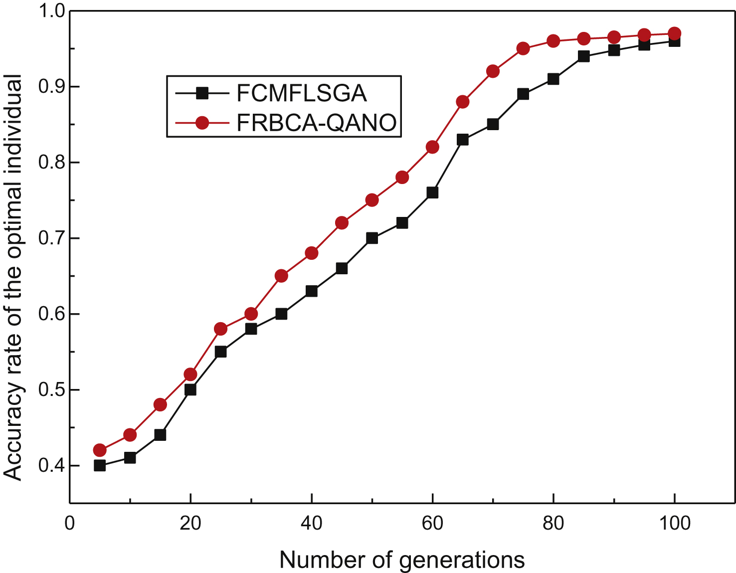
Fig.2
Rule number of the optimal individual with differentiterations.
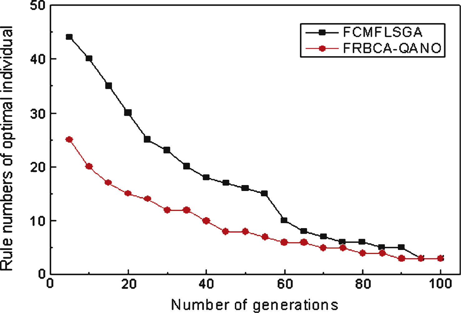
Table 1
Comparison of three algorithms
| Rule-based | FCMF- | FRBCA- | |
| classifier | LSGA | QANO | |
| Number of rules | 3 | 3 | 3 |
| Correct classification | 144 | 144 | 146 |
| Number of Variable | 2 | 1 | 1 |
| Accuracy | 96% | 96% | 96.7% |


