
Microbial control of river pollution during COVID-19 pandemic based on big data analysis
Abstract
Under the influence of epidemic situation, the treatment of pollutants is stricter. After the epidemic, how to treat the river pollutants by microorganisms has become a difficult problem. In this paper, the microbial treatment technology of water pollution was studied, and the water quality model was used to simulate the process of microbial degradation of river pollutants. The dynamic equation is used to describe the relationship among microbial proliferation, removal of organic pollutants, change of dissolved oxygen concentration, different forms of nitrogen and different forms of phosphorus, so as to realize the mathematical expression of water quality change in the process of microbial treatment of river pollutants. Finally, the numerical simulation model of microbial treatment of river pollution is obtained through experimental analysis, which provides an accurate reference model for the prevention and control of river pollution after the outbreak.
1Introduction
The novel corona virus pneumonia outbreak occurred worldwide in late 2019 and early 2020 [1, 2]. Under the influence of epidemic situation, the treatment of pollutants is stricter. After the epidemic, how to treat the river pollutants by microorganisms has become a difficult problem. In this paper, the microbial treatment technology of water pollution is studied, in order to obtain the numerical simulation model of microbial treatment of river pollution and provide an accurate reference model for the prevention and control of river pollution after the epidemic [3].
With the continuous development of industry and urbanization, the concentrated discharge of industrial waste-water and domestic sewage, the increasing load of organic carbon, organic nitrogen pollutants and phosphorus compounds in rivers, and the increasingly serious water pollution in urban rivers, it is particularly urgent to carry out research on river remediation technology [4, 5]. With the advantages of low energy consumption, low cost, good effect, easy operation, long duration and no secondary pollution, microbial remediation technology is the most promising main remediation technology [6]. In order to further explore the water quality migration process of microbial technology in river pollution control, this paper combines Monod microbial proliferation model with expanded activated sludge model EASM1, and Steeter-Phelps water quality model to numerically simulate the process of microbial degradation of river pollutants. Dynamic equations are used to describe microbial proliferation and removal of organic pollutants. In addition, combined with the change of dissolved oxygen concentration and the relationship between different forms of nitrogen and phosphorus, the water quality change in the process of microbial treatment of river pollutants can be expressed mathematically, so as to provide scientific basis for water quality prediction and process improvement in the process of treatment.
2Establishment of coupling model
2.1Model fundamentals
Organic pollution is widespread in major rivers in China, and non-point source pollution is increasingly prominent. According to statistics, more than 1 / 4 of rivers and river reaches in China cannot meet the requirements of the most basic irrigation water (Class V water quality standard in China) due to pollution. As far as the reach is concerned, the water pollution is serious and cannot be used for irrigation, that is to say, the reach inferior to class V accounts for about 10.6% [7]. The water body has lost its use value, and 46.5% of the river reaches are polluted equivalent to class IV and V [8].
(1) Monod model [9]. In 1942, French microbiologist Monod Jacques found that the growth curve of microorganism was similar to the biochemical reaction curve of living enzyme. On this basis, a Monod model describing the concentration of substrate and the growth rate of microorganism was proposed.
(1)
In the formula, μ is the growth rate of unit microbial biomass; μmax is the maximum specific growth rate of microorganisms; KS is the semi saturation coefficient; S is the concentration of substrate.
(2) EASM1 model [10]. One of the main technologies of microbiological technology is biological addition. The simulation of biological addition process needs to focus on the three processes of nitrifying bacteria enrichment culture, nitrification and denitrification in the main reactor. In 1986, the activated sludge model No.1 (ASM1) developed by the international water association was used to simulate the processes of carbon oxidation, nitrification and denitrification with good results. However, the ASM1 model does not contain the phosphorus removal process. if only ASM1 is used to model the biological addition, the change of phosphorus in the river course and the effect of biological addition on phosphorus removal cannot be simulated. EASM1 model is based on ASM1 and adds corresponding phosphorus removal process, which can simulate the changes of phosphate and phosphorus accumulating bacteria in the river course. Compared with ASM2 and ASM2 D, the dephosphorization part is simplified, the fermentation process, chemical precipitation process and denitrification dephosphorization process are omitted, and the model is simpler [11].
(3) Streeter Phelps water quality model [12]. The growth of microorganisms is not only limited by the growth substrate, but also affected by the change of dissolved oxygen, hydraulic conditions and flow hydrological conditions. Therefore, the improved S-P model is used to describe the law and expression of One-dimensional Steady-state River material transport [13].
(2)
(3)
2.2Development of dynamic equation of coupling model
By adopting the basic principle of self-purification and the equilibrium of activated sludge method, the numerical simulation in this study uses Monod dynamic equation developed in EASM1 model based on chemical oxygen demand COD as the equilibrium between microorganisms and other biodegradation processes. As the migration and diffusion processes in rivers are controlled by velocity gradient, the hydraulic model generated by longitudinal flow velocity is very important [14, 15]. Assuming that microorganisms and other variables change with water flow, the migration and diffusion term should be included in all dynamic equations. The mathematical expression of biodegradation process is as follows.
Concentration of easily biodegradable organic matter (SS) [16–22]:
(4)
Active hetero trophic biomass (XH):
(5)
The names, units and typical values of the above parameters are shown in Table 1.
Table 1
Representation of model dynamic parameters and correction results
| Symbol | Name | Units | Typical value | ||
| 10°C | 20°C | 17–18°C | |||
| Yh | hetero trophic yield coefficient | 0.67 | 0.67 | 0.67 | |
| Fp | Attenuation product coefficient | 0.08 | 0.08 | 0.08 | |
| ixb | Nitrogen coefficient in cells | 0.09 | 0.09 | 0.09 | |
| ixp | Nitrogen coefficient in attenuation products | 0.06 | 0.06 | 0.06 | |
| Ya | Yield coefficient of auto trophic bacteria | 0.24 | 0.24 | 0.24 | |
| μmax,H | Maximum specific growth rate of hetero trophic bacteria | d-1 | 3.00 | 6.00 | 12.00 |
| μmax,a | Maximum specific growth rate of auto trophic bacteria | d-1 | 0.30 | 0.80 | 0.80 |
| kh | Decay coefficient of hetero trophic bacteria | d-1 | 0.20 | 0.62 | 0.62 |
| bA | Attenuation coefficient of auto trophic bacteria | d-1 | 0.10 | 0.20 | 0.20 |
| KS | The half saturation coefficient of the solubles of hetero trophic bacteria | (COD) mg/L | 20.00 | 20.00 | 20.00 |
| KOh | Half saturation coefficient of dissolved oxygen in hetero trophic bacteria | (O2) mg/L | 0.20 | 0.20 | 0.20 |
| KNO3 | Semi saturation coefficient of NO3 production by hetero trophic bacteria under hypoxia | (NO-3- N) mg/L | 0.50 | 0.50 | 0.50 |
| KX | Half saturation coefficient of organic matter in hydrolysis process | g/g | 0.01 | 0.03 | 0.03 |
| KNH4 | Half saturation coefficient of dissolved oxygen in hetero trophic bacteria | mg/L | 1.00 | 1.00 | 4.00 |
| KO,a | The half saturation coefficient of dissolved oxygen in nitrobacteria | mg/L | 0.40 | 0.40 | 0.40 |
| kh | Maximum hydrolysis rate constant at 20 °C | g/g | 1.00 | 3.00 | 3.00 |
| ηg | Anaerobic hydrolysis rate constant of hetero trophic bacteria | 0.80 | 0.80 | 0.80 | |
| ηh | Correction factor for anoxic hydrolysis | 0.40 | 0.40 | 0.40 | |
| qPHA | Rate constants of PHA storage of polyhydroxyalkanoates | g/g·d | 2.0 | 3.0 | 3.00 |
| qPP | Rate constant of polyphosphate PP storage | g(PP) /g(PAO) d | 1.00 | 1.50 | 1.50 |
| μPAO | Maximum growth rate of PAO | d-1 | 0.67 | 1.00 | 1.00 |
| bPAO | Bacteriolysis rate constant of XPAO | d-1 | 0.10 | 0.20 | 0.20 |
| bPP | Decomposition rate constant of XPP | d-1 | 0.10 | 0.20 | 0.20 |
| bPHA | Decomposition rate constant of XPHA | d-1 | 0.10 | 0.20 | 0.20 |
| KO2 | Saturation coefficient of SO2 | g/m3 | 0.20 | 0.20 | 0.20 |
| Kss | Saturation coefficient of SS | g/m3 | 12.5 | 12.5 | 12.5 |
| KPS | Saturation coefficient of phosphorus stored in PP | g(P)/m3 | 0.20 | 0.20 | 0.20 |
| KP | The saturation coefficient of phosphorus in the growth process | g(P)/m3 | 0.01 | 0.01 | 0.01 |
| KPP | Saturation coefficient of polyphosphate | g(PP) /g(PAO) | 0.01 | 0.01 | 0.01 |
| KALK | Saturation coefficient of alkalinity | mol/m3 | 0.10 | 0.10 | 0.10 |
| KIPP | Inhibition coefficient of XPP storage | g(PP) /g(PAO) | 0.20 | 0.20 | 0.20 |
| KPHA | Saturation coefficient of PHA | g(PHA)/g(PAO) | 0.01 | 0.01 | 0.01 |
| KMAX | Maximum ratio of XPP/XPAO | g(PP) /g(PAO) | 0.34 | 0.34 | 0.34 |
| iPBM | Measurement coefficient | 0.20 | 0.20 | 0.20 | |
| vp | Measurement coefficient | 0.01 | 0.01 | 0.01 | |
| YPAO | Yield coefficient of polyphosphate bacteria (biomass /PHA) | g/g | 0.625 | 0.625 | |
| YPHA | PHA required for PP storage | g/g | 0.20 | 0.20 | |
| YPO4 | PP required for PHA storage | g/g | 0.40 | 0.40 | |
3Determination of model parameters and model solution
(1) Dispersion coefficient Ex. Many formulas can be used to simulate dispersion coefficients in rivers, such as McQuivey and Keefer, Fischer, Jain, Liu, Seo and Cheong, etc. This paper uses the most commonly used Seo and Cheong simulation formula.
(6)
(7)
(2) Reoxygenation coefficient K2. In this paper, the reoxygenation formulas of O’Connor and Dobbins are used to simulate:
(8)
(3) Pdepe solver in Matlab is used to solve the partial differential equations in the model.
4Case analysis
4.1Treatment measures
HX River is an east-west urban inland river on the west side of WAA Road in NC district, WX City, with a total length of 1.36 km and an upstream section with a water surface width of 4.5 m, water depth of 1.4 m and sludge of 1.6 m. The water surface of HX Bridge is 25 m wide, the water depth is 1.5 m and the sludge depth is 1.9 m. The downstream section is 7.5 m wide in water surface, 1.1 m deep in water and 1.2 m deep in sludge. The river directly receives the domestic sewage of surrounding residents. The sewage from 5 public toilets and 5 garbage transfer stations along the river all the year round and discharges about 10100 m of sewage directly into the river every day. In this paper, the improved numerical model uses the hydraulic data of the long, straight and regular trapezoidal channel, the river width is 25 m, the river bottom gradient is 0.00001 and Manning’s coefficient is 0.020. From November 12 to 13, 2018, according to the monitoring results of river water quality and the results of laboratory small-scale microbial acclimation, the cultured microbial agent (containing more than 3.0×10⁹ viable bacteria/ml) was diluted with river water in the proportion of 1:5, and added with promoter in the proportion of 1:1000, and then the diluted microbial agent was injected into the river bottom mud and river water with pump by plum blossom inoculation method. The inoculation range is 1.2 km from the upstream gate of the river to the box culvert of Wuai road in the middle and lower reaches. 250 kg of microbial agent is inoculated every 100 m, 120 kg of XL microbial accelerator product and 150 kg of culture medium are put in. Three times of inoculation were carried out. 9000 kg of native microorganism, 6000 kg of medium and 5000 kg of XL microbial growth promoting agent were used.
4.2Result analysis
The average monitoring data of 5 water quality monitoring points were used for simulation from November 12 to 23. The simulation results are shown in Fig. 1. From Fig. 1, we can get:
Fig. 1
Model simulation results.
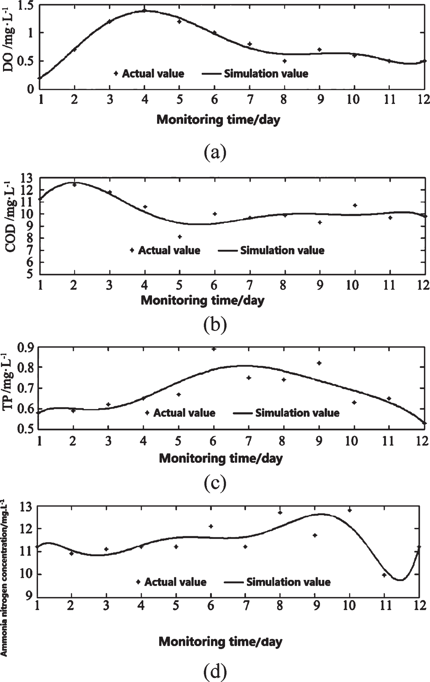
(1) The simulation results. In the first 4 days after microbial inoculation, microbial agents and additives were put into the river, and the manual operation was frequent. The river was affected by human disturbance and the DO concentration rose rapidly. The simulation results of Fig. 1 model were high. After 4 days inoculation, the disturbance weakened and the DO concentration gradually decreased. At this time, microorganisms multiplied and decomposed pollutants in large quantities. The water quality of the river was improved and the DO concentration slightly increased. However, due to the metabolism of microorganisms, the DO concentration fluctuated. The simulation results are ideal.
(2) COD simulation results. COD concentration increased two days before inoculation, which was caused by the continuous proliferation of microorganisms. At the beginning of the third day, due to the role of microorganisms, COD concentration decreased rapidly and finally became stable. The simulation results were ideal.
(3) TP simulation results. Due to the continuous injection of domestic sewage, the effect of microbial action on TP removal in water quality is not particularly obvious in the data, and the simulation value shows a slight upward trend and then downward trend. The simulation effect is better.
(4) Ammonia nitrogen simulation affection. Within 4 days after inoculation, the concentration of ammonia nitrogen tended to be stable, and on the fifth day, the concentration of ammonia nitrogen increased, which may be caused by a small amount of nitrogen element in the adjuvant.
In conclusion, the coupling model can be used to simulate the change trend of water quality in the river after microbial inoculation. Among the five monitoring points, the difference between the individual monitoring data and the simulated value is large, which may be caused by the accidental error during the field operation in the process of microbial inoculation, or by the indefinite discharge of domestic sewage of residents along the HX River. The overall simulation effect of the model is good.
5Conclusions
In this paper, for the first time, the extended model EASM1 based on the process of increasing phosphorus removal by ASM1 is coupled with Monod microbial proliferation model and Steeter-Phelps water quality model. The corresponding dynamic equations are put forward to simulate the change trend of DO, COD, TP and ammonia nitrogen in the process of treating pollution by microbial technology, and relatively ideal results are obtained. In this paper, the water quality index TP is added to the water quality prediction model module for the first time, and the dynamic equation describing its migration and transformation process is obtained, which expands the water quality prediction in the pollution control process and provides reliable basis for the development of water pollution control technology.
Because HX River did not completely cut off the pollution source in the treatment process and the accidental error in the process of artificial field operation, the water quality during the treatment was simulated, and the results showed that part of the simulation results were not ideal, and there was fluctuation phenomenon.
References
[1] | Lacey L.A. and Undeen A.H. , Microbial Control of Black Flies and Mosquitoes, Annual Review of Entomology 31: (1) ((1986) ), 265–296. |
[2] | Zahiri N.S. , Tianyun S. and Mulla M.S. , Strategies for the Management of Resistance in Mosquitoes to the Microbial Control Agent Bacillus sphaericus, Journal of Medical Entomology (3) 3. |
[3] | Munafò M. , Cecchi G. , Baiocco F. , et al., River pollution from non-point sources: a new simplified method of assessment, Journal of Environmental Management 77: (2) ((2005) ), 93–98. |
[4] | Kong X. , Zhang F. , Wei Q. , et al., Influence of land use change on soil nutrients in an intensive agricultural region of North China, Soil & Tillage Research 88: (1-2) ((2006) ), 85–94. |
[5] | Brown C.M. , Fry J.C. , Gadd G.M. , et al., Microbial Control of Pollution, Journal of Applied Ecology 30: (2) ((1992) ), 380. |
[6] | Pflug I.J. , Evaluating a Ground-Beef Patty Cooking Process Using the General Method of Process Calculation, Journal of Food Protection 60: (10) ((1997) ), 1215–1223. |
[7] | Kang H. and Vachtsevanos G. , Fuzzy hypercubes: Linguistic learning/reasoning systems for intelligent control and identification, Journal of Intelligent and Robotic Systems 7: (2) ((1993) ), 215–232. |
[8] | Xue S. , Intelligent system for products personalization and design using genetic algorithm, Journal of Intelligent and Fuzzy Systems 37: (1) ((2019) ), 1–8. |
[9] | Shapiro-Ilan D.I. , Microbial control of the pecan weevil, Curculio caryae, Southwestern Entomologist 27: ((2003) ), 101–114. |
[10] | Tanada Y. , Microbial Control of Some Lepidopterous Pests of Crucifers, Journal of Economic Entomology 49: (3) ((1956) ), 320–329. |
[11] | Lipa J.J. , Microbial control of mites and ticks, British Journal of Surgery 34: (136) ((1971) ), 434–434. |
[12] | Hammouda O. , Gaber A. and Abdelraouf N. , Microalgae and Wastewater Treatment, Ecotoxicology and Environmental Safety 31: (3) ((1995) ), 205–210. |
[13] | Liao S.W. , Gau H.S. , Lai W.L. , et al., Identification of pollution of Tapeng Lagoon from neighbouring rivers using multivariate statistical method, Journal of Environmental Management 88: (2) ((2008) ), 286–292. |
[14] | Liu Y. , Yang Y. and Xu C. , Risk Evaluation of Water Pollution in the Middle Catchments of Weihe River, Journal of Residuals Science and Technology 12: ((2015) ), S133–S136. |
[15] | Li X. , Zhang M. , Duan X. , et al., Effect of nano-silver coating on microbial control of microwave-freeze combined dried sea cucumber, International Agrophysics 25: (2) ((2011) ), 181–186. |
[16] | Kodama K. , Oyama M. , Lee J.H. , et al., Drastic and synchronous changes in megabenthic community structure concurrent with environmental variations in a eutrophic coastal bay, Progress in Oceanography 87: (1–4) ((2010) ), 157–167. |
[17] | Yao S. , Guo D. , Sun Z. , et al., A modified multi-objective sorting particle swarm optimization and its application to the design of the nose shape of a high-speed train, Engineering Applications of Computational Fluid Mechanics 9: (1) ((2015) ), 513–527. |
[18] | Zhen X. , Enze Z. and Qingwei C. , Rotary unmanned aerial vehicles path planning in rough terrain based on multi-objective particle swarm optimization, Journal of Systems Engineering and Electronics 31: (1) ((2020) ), 130–141. |
[19] | Guo X. , Ren H.P. and Liu D. , An Optimized PI Controller Design for Three Phase PFC Converters Based on Multi-Objective Chaotic Particle Swarm Optimization, Journal of Power Electronics 16: (2) ((2016) ), 610–620. |
[20] | Gomes H.M. , Multi-objective optimization of quarter car passive suspension design in the frequency domain based on PSO, Engineering Computations 33: (5) ((2016) ), 1422–1434. |
[21] | Omkar S.N. , Mudigere D. , Naik G.N. , et al., Vector evaluated particle swarm optimization (VEPSO) for multi-objective design optimization of composite structures, Computers & Structures 86: (1-2) ((2008) ), 1–14. |
[22] | Wu Y. , Li W. , Fang J. , et al., Multi-objective robust design optimization of fatigue life for a welded box girder, Engineering Optimization 2017: , 1–18. |

