
An ad-hoc network routing algorithm based on improved neural network under the influence of COVID-19
Abstract
Under the influence of COVID-19, an efficient Ad-hoc network routing algorithm is required in the process of epidemic prevention and control. Artificial neural network has become an effective method to solve large-scale optimization problems. It has been proved that the appropriate neural network can get the exact solution of the problem in real time. Based on the continuous Hopfield neural network (CHNN), this paper focuses on the study of the best algorithm path for QoS routing in Ad-hoc networks. In this paper, a new Hopfield neural network model is proposed to solve the minimum cost problem in Ad-hoc networks with time delay. In the improved version of the path algorithm, the relationship between the parameters of the energy function is provided, and it is proved that the feasible solution of the network belongs to the category of progressive stability by properly selecting the parameters. The calculation example shows that the solution is not affected by the initial value, and the global optimal solution can always be obtained. The algorithm is very effective in the prevention and control in COVID-19 epidemic.
1Introduction
Since December 2019, Wuhan City, Hubei Province has continued to carry out surveillance of influenza and related diseases. Multiple cases of viral pneumonia were found, all diagnosed as viral pneumonia/pulmonary infection. On January 12, 2020, the World Health Organization officially named it 2019-nCoV. On February 17, 2020, the Chinese Center for Disease Control and Prevention released the largest epidemiological analysis of new coronary pneumonia to date. Under the influence of COVID-19, an efficient Ad-hoc network routing algorithm is required in the process of epidemic prevention and control.
In recent years, with the development of modern communication technology, wireless network technology has become the focus of current research. Ad-hoc network is a multi-hop temporary autonomous system composed of a group of mobile nodes with routing and forwarding functions. It is mostly used in military tactical systems and some emergency systems such as flood rescue. In an emergency environment, users have put forward many new requirements for network quality of service (QoS), so efficient QoS support becomes more and more important.The research hotspots of QoS assurance in Ad-hoc networks are concentrated on QoS routing algorithms. The core problem is to optimize a certain parameter on the basis of satisfying the parameter constraints.
At present, routing mainly considers three kinds of calculation parameters: one is the additivity parameters, such as cost, delay, delay jitter and hop count. The second is multiplicative parameters, such as data loss rate. The third is to take small parameters, such as bandwidth. Reference [1] pointed out that when the constraints of routing include 2 or more additivity parameters, or include a combination of additivity and/or multipliability parameters, the route selection will be NP -Complete question.
ANN (Artificial Neural Net-works) is a parallel system composed of many nonlinear processing units. Since Hopfield and Tank pioneered the application of ANN to optimization calculations. ANN has become a powerful tool for studying the shortest path in large-scale networks. Literature [4] mainly discusses the application of two kinds of neural networks in information routing optimization. In document [5], LEE and CHANG applied ANN to study the communication routing problem of unreliable components. A Hopfield neural network was constructed in [6] to solve the shortest route problem in computer networks. These neural networks can make up for the defects of traditional routing algorithms, but the structure of neural networks is complex. Compared with traditional fixed networks, in Ad-hoc networks, the network topology changes more frequently. From the perspective of saving power, the node structure in the network should be as simple as possible. Therefore, how to design a suitable neural network model to adapt to the characteristics of the Ad-hoc network environment is still the focus of current research.
This paper mainly considers the routing problem that satisfies multiple constraints in Ad-hoc networks, that is, selects delay and cost as constraints, and selects cost as the optimization goal. A new Hopfield neural network model is established.
2Problem description
Most large-scale Ad-hoc networks are based on clustering structures. That is, the network is divided into multiple clusters according to the corresponding clustering strategy. Each cluster consists of cluster head nodes, gateway nodes and common nodes in the cluster [7, 8]. Communication between nodes in different clusters must be completed through the forwarding of gateway nodes between clusters. The Ad-hoc network is abstracted into a weighted undirected graph G(V,E*), as shown in Fig. 1.
Fig. 1
Energy function change.
The elements of set V are called nodes. The first node and the last node represent the source node and destination node in the Ad-hoc network, and the other nodes represent the gateway nodes in the network. The elements of the set E* are called edges, and Ei is used to represent the edge set from node i to node i + 1, where i,+1∈V. There may be multiple edges between two nodes, and Eji is used to denote the jth edge from node i to node i + 1. Its weight sequence < tij,cij>represents the delay and cost from node i to node i + 1 through the jth edge.
Introduce variables [9, 10]:
1 represents the j-th edge from node i to node i + 1 is selected as the route to the destination. 0 represents other.
Definition 1: The delay Mdelay and the cost Ncost of the route p = 1⟶ 2⟶... n-1⟶ n are defined as follows [11]:
Let T0 be the maximum network delay required. The minimum cost routing model that meets the delay requirements can be attributed to the following linear integer programming problem (LIP):
Equation (1) represents the minimum cost routing problem from node 1 to node n, that is, the objective function. Equation (2) ensures that the selected route meets the maximum delay constraint. Equation (3) ensures that only one edge is selected between any two adjacent nodes. Equation (4) is that the decision variable satisfies the integer constraint of 0,1.
3Algorithm
Neural network as a large-scale parallel algorithm, if it can be implemented on a parallel computer, its calculation speed will be greatly improved than the numerical solution. Since Hopfield and Tank proposed to use neural network to solve the traveling salesman problem (TSP) in 1986, people have been using this as an optimization method for various optimization problems. In many literatures, most of them use the TSP representation method (that is, the binary matrix) to find the shortest path and solve the routing problem and its sub-problems in the communication network. The output of the neural network corresponds to the solution of the problem. The output of each neuron is 0 or 1. This solution is called a binary solution or a discrete solution. In the method proposed in this article, the output of each neuron is Any real number on [0,1]. This output will also correspond to the solution of the problem to be solved, which is called a continuous Hopfield neural network (CHNN).
As a large-scale parallel algorithm, if the neural network can be implemented on parallel computer, its computing speed will be much faster than that of numerical solution. Since Hopfield and tank proposed to solve the traveling salesman problem (TSP) with neural network in 1986, they have been used as an optimization method for various kinds of optimization problems. In many literatures, they use the representation method of solving TSP (i.e. binary matrix) to find the shortest path with neural network to solve the routing problem or the sub problem in the routing problem in the communication network. The output of neural network is corresponding to the solution of the problem. The output of each neuron is 0 or 1, which is called binary solution or discrete solution. In the method proposed in this paper, the output of each neuron is any real number on [0,1], which also corresponds to the solution of the problem to be solved, This kind of neural network is called continuous Hopfield neural network (CHNN). Hopfield has many application fields, among which the algorithm research of network path is an important field.
In packet switched communication network or computer network (PSN), routing has an extremely important impact on the performance of the network. It is one of the main tasks that the network layer must complete. Therefore, finding a better routing algorithm has become a subject that people have been studying in recent years. According to the needs of different types of networks, the basis of routing is not the same. In terms of mathematical model, the objective functions to be optimized are different, such as network delay, cell loss rate, maximum output or reliability, etc. From the variables of objective function, it can be divided into two categories: one is to find the shortest path, the other is to allocate traffic. Now, we only take the average network delay in PSN as the optimization goal, and the variable is the traffic flow. In fact, this is a multi-commodity flow problem. There are many solutions to this kind of problem. The most common ones are Lagrange multiplier method, flow differential (FD) method and gradient projection GP method. The latter two methods are improved gradient reduction method. In this paper, FD method is improved, and neural network is used to solve the shortest path problem in each iteration.
3.1The mathematical model of routing
For a communication network or computer network whose topology g = g (V, l) and link capacity C=(CIJ) n×n have been determined, the M / M / 1 model can be used to calculate the link delay. It is assumed that the arrival rate of each service is consistent with the Poisson distribution, and the service demand between each end pair (i,j) has been calculated. It is represented by R=(Cij)n×n, where n is the number of ends of the network, and the maximum number of services in the whole network is W = n×(n-1), That is to say, there are w kinds of goods to be transmitted online. If the arrival of W kinds of services is independent of each other, according to the additivity of Poisson law, the total traffic on link L is
(1)
In this formula:
(2)
Where, l refers to the link, and its two ends are i,j, L(i,j) refers to all paths containing link l; x refers to the traffic volume of a certain service transmitted on path P. for each service w, there are Pw paths P can transmit, so there are constraints.
Rw is the service demand between source and destination pairs. The average delay of the whole network is [11]:
(3)
Here, CL represents link capacity. Routing problem can be summed up
(4)
It should be noted here that Dl is a second-order differentiable continuous function on [(0,c l), and its first derivative can be expressed as:
(5)
Therefore, T is a convex function of Fl,. since link flow Fl is a linear function of path flow xp, formula (2) is a convex function with path flow as a variable and convex constraint set
3.2CHNN algorithm
According to the characteristics of neural network, the output function of neuron is nonlinear, and the interval of function value is (0,1).
Here, take the output function:
(6)
the solution of the factor x* ∈ [0, ∞)), and make The output of the neuron corresponds to the solution of formula (2), and the variables in formula (2) need to be transformed to make the output solution of the neural network
(7)
then formula (2) can be noted as:
(8)
(9)
The energy function of Hopifeld neural network can be established by formula (2)
(10)
In formula (6), item a corresponds to the objective function in formula (3), and item B corresponds to formula (4). Since the output of neurons is all non negative, formula (5) is naturally satisfied. According to the conclusion in the literature, the value of energy function decreases with the continuous updating of neuron state. If the minimum value of item B is 0. When e is very small, a will be very small. That is to say, it corresponds to the solution of formula (3). It has been analyzed that if formula (L) is a convex function, then item a in formula (6) is a convex function, so it is not difficult to prove that item B is also a convex function, then E is a convex function. Therefore, the stable output of the neural network will be the global optimal solution of formula (3), and the individual solutions will not be affected by the initial value. The solution of formula (3) can be obtained by randomly selecting a set of initial values.
Therefore, according to the relationship between the equation of state renewal and the equation of energy function changing with time, as well as Equation (6), the following equation can be derived:
(11)
(12)
In this equation:
(13)
(14)
3.3Path search algorithm
In fact, if you want to implement the FD, GP, and CHNN algorithms, you need to search all feasible paths for each service to get the path set P of the entire network. In addition, the algorithm can also be used to solve the shortest path in a network where all link values are equal.
For the directed connected graph G=(V,L), V is the node set, which is expressed by the formula. L is a set of directed links, expressed by the formula. The connection matrix of graph G can be expressed by the formula C=(cij)n ×n.
(15)
Here, the length of the path is defined as the number of directed links, O is the source end, D is the sink end, and the path set is Pl, then the path search algorithm between ODs is as follows:
(16)
(17)
3.4QoS routing calculation based on Hopfield neural network
Hopfield neural network is formed by interconnecting multiple neurons according to symmetrical weight coefficients. Its basic idea is to construct an appropriate energy function and convert the solved optimization problem into a minimum value of energy function. Therefore, the energy function is the key to the design of Hopfield neural network, it reflects the goal of solving the problem, and is the basis for constructing the dynamic process of the network.
The general form of the energy function of the Hopfield neural network is
(18)
The dynamic characteristics represented by the i-th neuron are:
(19)
(20)
Among them, yi,xi∈ {0,1}, hi respectively represent the input, output and deviation of the i-th neuron, and wij is the connection weight from neuron j to neuron i (wij = wji). Equations (6) and (7) satisfy the differential equations of Hopfield neural network [2, 3]:
(21)
(22)
According to formula (8) and formula (9), Can be exported as:
(23)
This makes the energy function E of the Hopfield neural network gradually stabilize. The N-dimensional space {0,1} N is called hypercube, and x∈{0,1}N is the space vertex. A Hopfield neural network was constructed in [6] to solve the shortest route problem in computer networks.
(24)
(25)
(26)
Among them, cij represents a unit cost, aij represents the quality of xij, and bi represents the overall quality requirement for i. Its energy function is as follows:
Among them,
However, it is not suitable for the Ad-hoc network whose network topology changes frequently. Because the cost-related part (item 4) in E1 is a quadratic, its minimization process greatly depends on the network connection weight coefficient. In this way, the instability of the network cost due to frequent changes in the topology of the Ad-hoc network will affect the minimization process of E1, and the neural network determined by E1 needs to add additional neurons, that is, the relaxation of the energy function in the second Variables make the structure of the neural network complicated. To this end, a new energy function is constructed as follows:
(27)
(28)
(29)
Theorem 2: If the parameters of the Hopfield network energy function E, A and B meet the conditions:
(30)
(31)
which is, if
(32)
When xsj = 1, then
(33)
The above situation can be obtained, when, A > C/2 + (D/2) × CM, B > (C - D)/2, Infeasible solutions are unstable.
If the parameters C and D of the Hopfield network energy function E satisfy the conditions: C > DCM, then the feasible solution is asymptotically stable, otherwise it is unstable.
Due to
(34)
When the parameters of the Hopfield neural network energy function E meet the conditions:
According to Theorem 2 and Theorem 3. Differential equations based on Hopfield neural network
(35)
In order to speed up the algorithm convergence, when each node has an edge corresponding to xij greater than 0.5, the algorithm ends. At this time, take:
(36)
4Case analysis
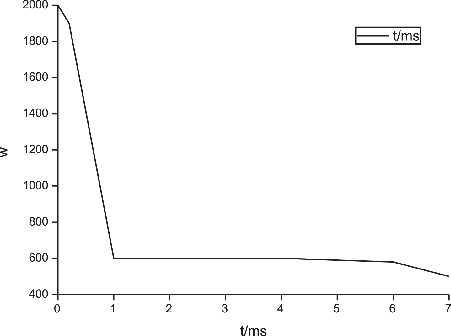
It is required to find a minimum cost route from node 0 to node 4 that satisfies the delay not exceeding 21 ms. According to the above neural network algorithm, the network parameters A = 2 000, B = 400 000, C = 400, D = 10, the initial values of xij are all 0. The final result of the operation is shown in Table 1, and Fig. 1 is the change graph of the energy function.
Table 1
Result of the instance(xij)
| Side | Node | |||
| 0 | 1 | 2 | 3 | |
| 0 | 0.63235301 | 0.23421053 | 0.16646238 | 0.22849746 |
| 1 | 0.36070254 - | –0.03743995 | 0.70976333 | 0.22849746 |
| 2 | / | –0.03743995 | –0.10518809 | 0.50014793 |
| 3 | / | 0.77751147 | 0.16646238 | / |
It can be seen from Table 1 that the minimum cost routing that meets the QoS requirements is x00 = 1, x13 = 1, x21 = 1, x32 = 1, and the rest xij = 0. The cost at this time is 8, and the delay is 20 ms. It can be seen from that the neural network converges quickly.
5Conclusions
Under the influence of COVID-19, an efficient Ad-hoc network routing algorithm is required in the process of epidemic prevention and control. Hopfield neural networks are increasingly becoming an important way to solve large-scale optimization problems with their powerful parallel processing capabilities. According to the characteristics of Ad-hoc network, this paper presents a new Hopfield neural network, which is used to solve the minimum cost problem of Ad-hoc network under the delay requirement. The neural network has a simple structure and can be applied to a network environment with frequent topology changes. The relationship between the parameters of the energy function is determined to ensure that the feasible solutions to the problem are asymptotically stable. This neural network converges to a stable and feasible solution in theory, and the simulation results show that it converges to the optimal solution of the system at a faster rate. It can be seen from the mathematical model in this paper that the calculation of routing can be easily extended to solve the routing optimization problem based on multiple parameter constraints, just add the parameter constraints to the constraints of the model. It can be seen that the models and algorithms proposed in this paper have certain practical significance for Ad-hoc networks and QoS routing in the prevention and control during COVID-19 epidemic.
References
[1] | Yanez-Marquez C. , Lopez-Yanez I. , Camacho-Nieto O. , et al., BDD-based algorithm for the minimum spanning tree in wireless ad-hoc network routing, IEEE Latin America Transactions 11: (1) ((2013) ), 600–601. |
[2] | Chauhan Jyoti , Minimized routing protocol in ad-hoc network with quality maintenance based on genetic algorithm: a survey, Evolutionary Ecology Research 9: (6) ((2013) ), 1023–1041. |
[3] | Wang J. , Osagie E. , Thulasiraman P. , et al., HOPNET: A hybrid ant colony optimization routing algorithm for mobile ad-hoc network, Networks 7: (4) ((2009) ), 690–705. |
[4] | Nancharaiah B. and Chandra Mohan B. , The performance of a hybrid routing intelligent algorithm in a mobile Ad-hoc network, Computers & Electrical Engineering 40: (4) ((2014) ), 1255–1264. |
[5] | Kwon O.C. , Oh H.R. , Lee Z.K. , et al., Entire network load-aware cooperative routing algorithm for video streaming over mobile Ad-hoc networks, Wireless Communications and Mobile Computing 13: (12) ((2013) ), 1135–1149. |
[6] | Sivakumar R. , Sinha P. and Bharghavan V. , CEDAR: a core-extraction distributed Ad-hoc routing algorithm, IEEE Journal on Selected Areas in Communications 17: (8) ((1999) ), 1454–1465. |
[7] | Rubin I. and Zhang R. , Robust Throughput and routing for mobile ad-hoc wireless networks, Networks 7: (2) ((2009) ), 265–280. |
[8] | Miao X. and Deng M. , DCEEMR: A delay-constrained energy efficient multicast routing algorithm in cognitive radio ad-hoc networks, International Journal of Distributed Sensor Networks 2014: ((2014) ), 1–10. |
[9] | Lee S.H. , Choi E. and Cho D.H. , Timer-based broadcasting for power-aware routing in power-controlled wireless ad-hoc networks, IEEE Communications Letters 9: (3) ((2005) ), 222–224. |
[10] | Dricot J.M. , Ferrari G. and Doncker P.D. , Cross-layering between physical layer, medium access control, and routing in wireless ad-hoc networks, and Ubiquitous Computing 9: (3) ((2012) ), 159–170. |
[11] | Panichpapiboon S. , Ferrari G. , Wisitpongphan N. , et al., Route reservation in ad-hoc wireless networks, IEEE Transactions on Mobile Computing 6: (1) ((2007) ), 56–71. |

