
Enhancing shallow water quality monitoring efficiency with deep learning and remote sensing: A case study in Mar Menor
Abstract
Satellite remote sensing technology has proven effective in monitoring various environmental parameters, but its efficiency in assessing shallow lakes has been limited. This study applies state-of-the-art machine and deep learning algorithms supported by classical statistic methods to analyze remote sensing data to measure chlorophyll-a (Chl-a) concentration levels. Focused on a shallow coastal lagoon, Mar Menor, this work analyzes statistically daily Sentinel 3 information behaviour and compares Machine Learning and Deep Learning techniques to enhance efficiency and accuracy data of this satellite. Convolutional Neural Networks (CNNs) stand out as a robust choice, capable of delivering excellent results even in the presence of anomalous events. Our findings demonstrate that the CNN-based approach directly utilizing satellite data yields promising results in monitoring shallow lakes, offering enhanced efficiency and robustness. This research contributes to optimizing remote sensing data to and produce a continuous information flow addressed to monitoring shallow aquatic ecosystems with potential environmental management and conservation applications.
1.Introduction
Satellite Remote Sensing (SRS) is rapidly emerging as a dominant technology for monitoring diverse natural environments [24,30]. The variety of sensors on satellites allows to capture and record different physical Earth events. They producing high-resolution images and/or datasets, characterized by precise geometric accuracy and detailed radiometric information which allow the analisys of biogeophysical parameters [42,45,49] to provide a wide range of products to depict the land, oceans, and beyond [26]. Technological advancements have ushered in superior spatial and temporal resolutions, offering new service opportunities such as ESA’s Sentinels [32] and NPP VIIRS [27] products. Despite SRS provides worldwide information, still it needed to be adapted to regional or local characteristics, thus leading to discrepancies between satellite-derived metrics and actual surface parameters [48].
This situation highlights concerns about accuracy. While in situ samples are considered the gold standard due to their lower measurement errors, they are difficult to obtain, especially in marine environments. The main disadvantages of in situ sampling include significant time and financial costs for frequent data collection, the need for specialized personnel, and the limitation to measuring specific parameters. Additionally, the variation in measurement methods used by different organizations can result in inconsistencies. This is compounded by a significant gap in spatial and temporal uniformity in data collection [35]. Despite its potential precision trade-off compared to in situ approaches, remote sensing counterbalances many field methods limitations. Its cost-effectiveness and the regularity of observations render it indispensable for longitudinal water quality surveillance.
Fig. 1.
In situ monitoring points (ISMP) undertaken by the Regional Government of Murcia (CARM) in the Mar Menor.
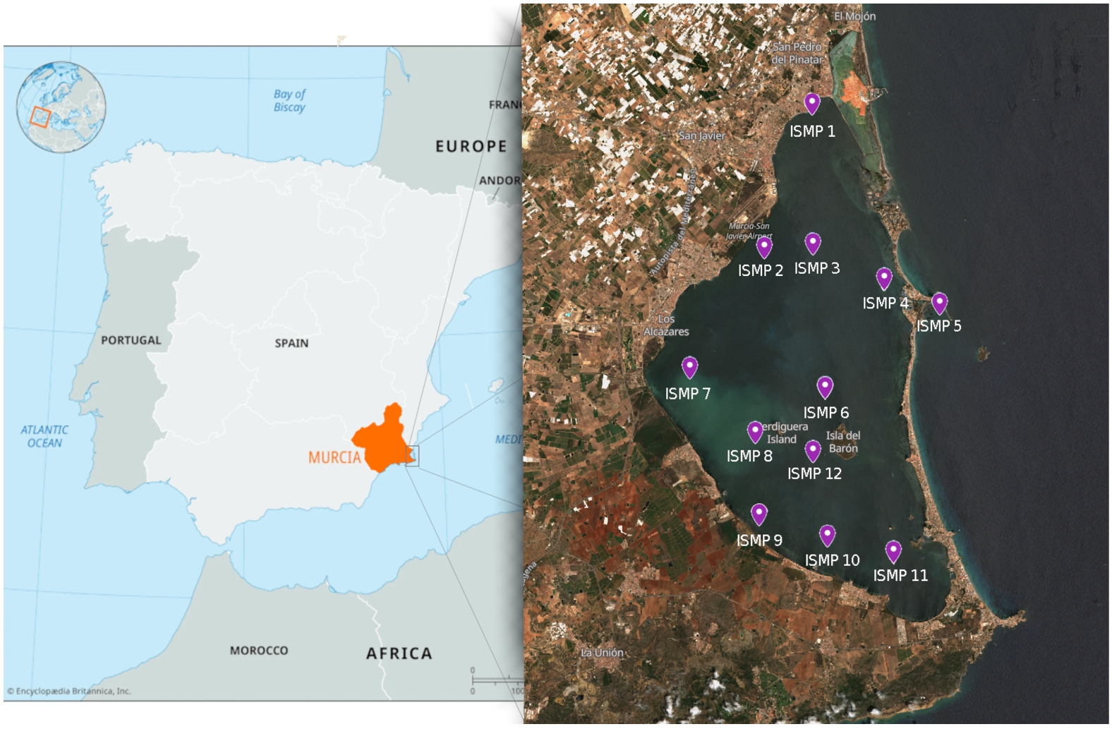
Taking advantage of the potential of SRS data we focus on the Mar Menor lagoon in Murcia, Spain, which faces significant water quality issues from various sources [40]. Situated in Murcia (Southeastern Spain), the Mar Menor is the largest coastal lagoon on the Iberian Peninsula and ranks among the biggest in Europe, spanning an area of 135 km2. Characterized by its relatively shallow depth, it averages 3.6 m and peaks at 7 m. The lagoon is separated from the Mediterranean Sea by a 22 km sandy barrier, La Manga, interspersed with several gullies. These gullies provide the lagoon with its semi-confined nature, bestowing its distinctive temperature and salinity attributes (refer to Fig. 1). Beyond its environmental significance, the Mar Menor plays a crucial role in Murcia’s economy. It draws tourists, recreational enthusiasts, and fishermen alike, courtesy of its unique climatic conditions and rich natural resources. Furthermore, the Mar Menor basin, known as Campo de Cartagena (CC), spans over 1,200 km2. This extensive plain is interspersed with ephemeral streams that collect the region’s infrequent yet intense rainfalls [41]. Historically, the Mar Menor’s pristine, transparent waters symbolized its resistance to eutrophication. Yet, the last decade has witnessed the lagoon’s shift towards eutrophic tendencies [7] due, mainly, to increasing anthropogenic pressures, such as agriculture and tourism, which have led to several ecological crises and brought it to the brink of collapse. This shift owes largely to modifications in the CC’s agricultural practices, including the advent of intensive irrigation. Consequently, the lagoon has seen an influx of nutrients, particularly nitrates and other fertilizing agents, leading to an upsurge in pollution and eutrophication [15,25]. The 2016 extreme eutrophication incident is a testament to this degradation, marking a notable decline in water transparency and quality [34]. Subsequent events, such as the 2019 spike in Chl-a levels after a storm, further accentuated the lagoon’s vulnerability [39]. In light of these challenges, proactive intervention is imperative. Thus, the importance of Chl-a concentration is a pivotal metric indicative of the eutrophication status of the Mar Menor ecosystem and the developing of satellite-based monitoring system to provide a lagoon health surveillance as continuous as possible.
Numerous studies have explored the potential of Satellite Remote Sensing (SRS)-based monitoring systems for Chlorophyll-a (Chl-a) concentrations, particularly in shallow water environments. However, these environments present specific challenges. Despite significant works such as [17,31] demonstrating a correlation between Chl-a and certain spectral bands (blue, green, red, and Near-Infrared), this methodology does not adapt well to shallow waters. Moreover, this technique commonly employs the Moderate Resolution Imaging Spectroradiometer (MODIS) instrument from the Terra and Aqua missions, which are now considered outdated. Other studies have enhanced satellite data by applying machine learning techniques, as evidenced by [1,6,28,47]. These studies validate and highlight the use of satellite data in various water environments, yet they do not propose specific models to estimate Chl-a. For instance, [1] developed algorithms for Sentinel 3 atmospheric corrections and highlight the appropriate use of Sentinel 3 in shallow lakes to analyze its quality. Moreover, [6] proposes an interesting approach, but a somewhat imprecise, using machine learning with Landsat 8 data.
Furthermore, owing to the recent notoriety of the Mar Menor, studies based on this environment, such as [5,11,19,20], provide insightful approaches using Landsat 8/9 and Sentinel 2 missions. [5,11] validate the use of remote sensing in the Mar Menor, while [19,20] offer algorithms for Chl-a estimations among other variables, employing Landsat 8/9 and Sentinel 2 or a combination thereof. Despite [20] achieved notable results, it is essential to recognize that their analysis was based on a dataset interpolated to bridge data gaps. These gaps were primarily due to the four-day revisit time of Sentinel 2, compounded by the presence of invalid images and the necessity of synchronizing with in-situ data occurrences. Employing Landsat extends this interval even further. Although Landsat 8/9, Sentinel 2, or their combination are frequently utilized for studying small and consequently shallow lakes, owing to their high resolutions, they encounter challenges due to extended periods without data, an issue that can be effectively addressed by utilizing the twin Sentinel 3 satellite, which provide daily data. The Mar Menor, despite its shallowness, is expansive. Therefore, studies conducted in environments similar to ours, such as the research on the western shallow part of Lake Erie referenced in [37], demonstrate that Sentinel 3 data is a promising candidate for analyzing cyanobacterial blooms related to Chl-a. This concept is further reinforced by [29]. However their analysis, which utilizes Sentinel 3 for monitoring small inland lakes, also encounters several challenges. These include substantial errors associated with derived remote sensing reflectances and pigment concentrations. Such complexities in modelling are crucial when considering the unique ecological context of the Mar Menor. The challenges are multifaceted, including a lack of high-quality in-situ data, spatial disparities between in-situ measurements and remotely sensed pixels, oversight of the intrinsic heterogeneity of terrestrial and marine surfaces contributing nutrients to the lagoon, and theoretical gaps relating to scale discrepancies during validation. Furthermore, there is a prevailing assumption regarding the unfettered reliability of data from satellite systems, often overlooking rigorous validation processes and comprehensive coverage spanning the spectrum of available products.
Consequently, Sentinel 3 emerges as a remarkable option for the consistent and dependable monitoring of Chl-a levels in the unique physical environment of Mar Memor and as pivotal aspect of its aquatic health research. Its data proves indispensable in Mar Menor, offering comprehensive large-scale insights. This facilitates informed decision-making processes, underpinned by robust Chl-a forecasting capabilities.
2.Research aim
Our monitoring system proposal extends research [16] that utilizes Sentinel 3 and its OLCI instrument for Chl-a estimation based on daily data. This study highlights the necessity of evaluating the precision of in-situ data against data derived from satellites. The focus is on several in-situ measurement points (ISMPs). Considering the variable and unpredictable nature of this data, the system aims to derive a Chl-a metric from satellite data with minimal error. This approach enables stakeholders to effectively monitor water quality changes and intervene in a timely manner to prevent critical degradation. The proposed mechanism for Chl-a monitoring includes a range of models to enhance the accuracy of data obtained from the Copernicus ocean monitoring framework, with a primary focus on Chl-a data sets from twin Sentinel 3 which is able to provide daily information. Our study begins with the development and evaluation of a classical statistical model, tailored to the unique environmental conditions of Mar Menor and its inherent data variability, influenced by ecosystem-specific factors like bottom vegetation density [18]. We conduct an extensive classical statistical analysis to understand these system dynamics, which forms the basis for further data interpretation and modeling. In the initial stages, our analysis includes examining autocorrelation in predictor variables, identifying relationships between data points over specific time intervals, and eliminating variables with low model tolerance. We use the Durbin–Watson test [9] to detect autocorrelation in our regression analysis residuals. To evaluate the effectiveness of the classical model, we compare it with machine learning and deep learning approaches, determining its predictive capacity and identifying the most suitable model for our monitoring system. We also consider modifying some constraints of the classical model, focusing on incorporating more selective variables to reduce noise and enhance predictive accuracy. By integrating machine learning, deep learning, and classical statistical methods, we aim to develop an advanced model that includes both established and novel measurement points. This comprehensive approach leads to the creation of a predictive framework specifically designed for the monitoring system we envision.
The primary contributions of this study include the following:
– SRS data analysis using classical statistics, discerning behaviors within such ecosystems and pruning non-essential data and variables for an optimized predictive model.
– Comparing machine learning (ML) and deep learning (DL) models with classical statistical approaches for estimation of chlorophyll-a (Chl-a) concentration in the Mar Menor. This comparison is based on comprehensive data sets, further refined using insights from the Durbin–Watson test.
– Exploration of alternative variable selection methodologies, particularly by easing the constraints imposed by the Durbin–Watson test, leading to the formulation of revamped ML and DL models based on this refined data set.
– Establishment of a comprehensive model for Mar Menor to estimate Chl-a which facilitates continuous monitoring of lagoon health and augments the ability to pinpoint peak Chl-a concentrations. It will provide large series to work in forecasting.
The remainder of this article is organized as follows: Section 3 details the materials and methods implemented in this study. In Section 4, we present the quantitative findings derived from all SRS-based products tailored for monitoring the Mar Menor coastal lagoon. Conclusions and potential directions for future research are outlined in Section 6.
3.Materials and methods
This section comprehensively details the materials and methods employed in our research. It first describes the dataset utilized in this study, encompassing both in-situ and Satellite Remote Sensing (SRS) data. This is followed by a brief description of the various models implemented in this research.
3.1.In situ data
The data used in this study, provided by the Regional Government of Murcia (CARM), are essential for analyzing remote sensing data. These data are from August 2016, a period marking the onset of Mar Menor’s degradation, prompting CARM to initiate regular monitoring activities. The compiled dataset includes almost weekly measurements taken at various depths across twelve points in Mar Menor, designated as in situ measurement points (ISMPs). These ISMPs represent the lagoon’s heterogeneity, characterized by diverse attributes such as depth and proximity to critical landmarks like the shoreline and wadis. Table 1 details the data provided by CARM, encompassing variables like chlorophyll-a (Chl-a), turbidity, chromophoric dissolved organic matter (CDOM), oxygen, salinity, and pH. However, due to its significant correlation with anoxia episodes, our study primarily focuses on Chl-a.
Table 1
Overview of the in situ monitoring data by CARM
| In situ data source | CARM |
| Sampling starting date | 2016-08-02 |
| Sampling end date | 2022-02-24 |
| #Samples | 3,251 |
Table 2
Statistical description of the Chl-a data sourced from CARM
| Depth (m) | Chl-a (mg/l) | |
| Count | 6146 | 6146 |
| Mean | 2.225 | 2.651 |
| Std | 1.66 | 3.865 |
| Min | 0 | 0.022 |
| 25% | 1 | 0.726 |
| 50% | 2 | 1.367 |
| 75% | 4 | 2.964 |
| Max | 6 | 28.112 |
The dataset is pre-filtered, which obviates the need for additional data cleaning or outlier identification in our study, thereby ensuring a higher degree of reliability. In our research methodology, we categorize data based on depth to facilitate more precise analytical clarity. As a result, our data interpretations and model fittings are tailored to specific depth intervals, thus mitigating any potential confusion. For instance, in our analysis, measurements recorded at depths ranging from 0 to 1 meter are classified under ‘depth 0’, while those from 1 to 2 meters are labeled as ‘depth 1’, and so forth. Table 2 offers an in-depth exploration of the Chl-a data characteristics, encompassing statistical metrics such as count, mean, standard deviation, and distribution percentiles.
3.2.Satellite Remote Sensing data
SRS has risen in prominence as a near real-time (NRT) monitoring tool, addressing both natural and societal challenges. Its significance spans regional to global scales, supporting several global initiatives such as the Sendai Framework, Paris Agreement, and Sustainable Development Goals [21,36,46].
This paper utilizes publicly available satellite remote sensing (SRS) data from the European Copernicus Marine Service (CMS). The CMS offers extensive information on oceanic conditions at both global and regional scales. Among the various products provided by Copernicus, our study specifically concentrates on data from the Sentinel 3 A and B satellites. Both satellites are equipped with the Ocean and Land Colour Instrument (OLCI), which provides data across 21 spectral bands and boasts a maximum spatial resolution of 300 meters. The unique twin-satellite system of Sentinel 3 A and B enables daily revisits to the same region at approximately the same hour. These characteristics make Sentinel 3 exceptionally suited for daily water monitoring, as they obviate the need for image calibration at different times, while providing sufficient spatial resolution. CMS processes OLCI data to offer a range of products tailored to diverse research objectives. This study utilizes data from the Level-2 Water Full Resolution (OL_2_WFR) products, which provide surface directional reflectances. These are corrected for atmospheric effects and sun specular reflection, and include two Chlorophyll-a (Chl-a) concentrations measured in milligrams per cubic meter (mg/m3.), computed using the OC4Me and Neural Network algorithms. The Level 2 (L2) products also include other parameters derived from these spectral bands, such as Total Suspended Matter concentration (TSM) and the Diffuse Attenuation Coefficient for down-welling irradiance (KD490). While these parameters offer insights into water quality aspects like turbidity or transparency, they are beyond the initial scope of this research. In terms of Chl-a concentration, our study leveraged the Inverse Radiative Transfer Model-Neural Network (IRTM-NN) due to its capability to handle negative reflectance values, a challenge for conventional algorithms. The IRTM-NN, pre-trained by CMS, uses neural networks for efficient computation and outputs various water-inherent optical properties. For a comprehensive understanding, readers are directed to [38]. Furthermore, the OL_2_WFR ancillary information includes flag data indicating the nature of each pixel, categorizing them as land, water, snow, cloud, invalid, and others. For this study, only pixels labeled as ‘water’ were considered, with invalid entries being disregarded.
It is important to highlight that CMS publishes products based on processed time. Thus, we prioritize Non-Time Critical (NTC) files, which are released 24/48 hours post-satellite data acquisition, offering a more refined and accurate dataset compared to Near Real-Time (NRT) products. Integrating a monitoring system can begin with NRT data and be updated once the NTC dataset becomes available. The CREODIAS platform offers both a web interface and an Application Programming Interface (API) for accessing and downloading Sentinel 3A/B products, as well as data from other satellite sources [33]. Utilizing its API, our study acquired several netCDF4 files for the specified ISMPs and study dates. These files were instrumental in extracting the parameters mentioned previously: Chl-a concentrations and reflectances.
Unlike deeper waters, the challenges associated with SRS in shallow waters are multifaceted and complex, encompassing issues such as water clarity, bottom reflectance variability, and the intricate interplay of light within these environments. Thus, reflectances from shallow waters combines the water column and seabed reflectance. Also, the optical properties of shallow waters are often influenced by a higher concentration of suspended sediments, organic matter, and other particulates. These elements can scatter and absorb light differently than clear open-ocean water, leading to skewed measurements when interpreted by algorithms primarily designed for deeper waters. This blending complicates the spectral signature, making it difficult to discern and isolate particular water quality parameters and can lead to rapid changes in water quality parameters, potentially outpacing the satellite’s revisit rate and thus missing short-term but significant events.
There is also the challenge of spatial resolution. While a 300-meter resolution might be appropriate for vast open oceans, it may fail to capture the fine-scale variability present in smaller, shallow water bodies, where features like seagrass beds, coral reefs, or algal mats can drastically change over short distances. Given these challenges, it is evident that while satellites like Sentinel 3 are invaluable for broad-scale, open-ocean observations, they may fall short in delivering precise data for shallow waters. This emphasizes the imperative need to integrate satellite observations with in-situ measurements and other data sources, harnessing complementary strengths to ensure a comprehensive and robust monitoring system.
An Initial analysis indicates a moderate correlation between Sentinel 3 Chl-a values and CARM in-situ measurements (see Section 4). The correlation quality varies by ISMP, suggesting that S3 data might not be uniformly reliable across all points. Moreover, the Sentinel 3 dataset lacked identifiable Chl-a peaks, underscoring potential limitations in pinpointing algal blooms that were evident during the study period.
3.3.Working datasets
By grouping the previous dataset described, for this research, we generate distinct datasets for each ISMP, consisting of paired Sentinel 3 A/B data and corresponding in-situ measurements, organized by date. These datasets contain dimensionless reflectances for each ISMP location as input variables and in-situ Chl-a concentrations measured in mg/m3. Table 3 summarizes the number of instances for each dataset. Based on findings from [16], we excluded ISMPs 1, 5, and 9 from our study. Their exclusion was primarily due to the shallow nature of their waters and the lower quality of data derived from these locations, rendering them unsuitable for our monitoring framework.
Table 3
Number of instances by ISMP and depth
| ISMP | Depth | ||||||
| 0 | 1 | 2 | 3 | 4 | 5 | 6 | |
| 2 | 105 | 105 | 105 | 105 | 105 | 98 | |
| 3 | 108 | 108 | 108 | 108 | 108 | 108 | 42 |
| 4 | 112 | 112 | 112 | 112 | 112 | 30 | 4 |
| 6 | 103 | 103 | 103 | 103 | 103 | 103 | 46 |
| 7 | 108 | 109 | 109 | 108 | 106 | ||
| 8 | 103 | 103 | 103 | 103 | 102 | ||
| 10 | 98 | 99 | 99 | 99 | 99 | ||
| 11 | 104 | 104 | 105 | 103 | 54 | ||
| 12 | 101 | 101 | 101 | 101 | 101 | 98 | |
3.4.Calibrating remote sensing to Chl-a measurements
In this article, we tackle Chl-a estimation through a regression analysis framework. Our primary objective is to establish a relationship between satellite-derived data and corresponding in-situ Chl-a measurements. Significantly, our exploration extends beyond traditional statistical regression methods to include modern Machine Learning (ML) models. This dual approach enables a comparative analysis of conventional statistical techniques and state-of-the-art ML methodologies, assessing their robustness and effectiveness. Focusing on the SRS data obtained from the CMS, particularly for the Mar Menor region, our goal is to determine which approach – traditional or contemporary – offers superior accuracy and predictive capability in Chl-a forecasting. To achieve this, we have carefully curated a range of both statistical and ML algorithms for thorough evaluation, as well as the ERROS AND IT PARAMETER.
3.4.1.Algorithms
– Linear Regression (LR): This traditional statistical method models the relationship between a dependent variable y and one or more independent variables x. It’s used for both simple (one independent variable) and multiple regression (more than one independent variable) scenarios [10].The general form of the model for multiple linear regression with p predictors is:
where– Random Forest Regression (RFR): An effective supervised ensemble learning method that integrates multiple decision trees to produce a final prediction. Each tree is created using a portion of the training data with bootstrapping and considers a random subset of features for splitting, enhancing diversity and reducing overfitting. RF’s bagging approach ensures varied tree perspectives, leading to robust predictions. It aggregates tree outputs, usually by averaging, to form the final prediction. RF is particularly adept at determining feature importance, handling outliers, and dealing with non-linear data. It resists the curse of dimensionality, making it effective even with numerous features. The ensemble nature of RF balances individual tree errors, yielding a model with better generalization and reduced variance [3].
– Decision Tree Regressor (DT): Using for regression, DT predicts continuous values by constructing a tree where each node represents a test on a feature and each leaf node contains the predicted output value. The common criterion for splitting in regression is the Residual Sum of Squares (RSS), which measures the total variance of the output variable about its mean for the instances at a given node.
where– K-Nearest Neighbors Regressor (KNN): KNN operates on the principle of feature similarity and predicts the output of a new instance by averaging the output values of its k nearest neighbors. The predicted output
whereKNN’s key advantage is its non-parametric approach, effectively handling complex, non-linear data relationships without presuming a specific data form. However, its need to retain the entire training dataset for predictions leads to high memory usage and slower performance with large datasets. The choice of distance metric and the k value are critical for its accuracy. Additionally, due to its reliance on distance calculations, feature scaling is essential for optimal performance, emphasizing the importance of preprocessing in KNN applications. This method balances flexibility in modeling with considerations for memory and computational efficiency [22].
– Multi-layer Perceptron Regressor (MLP): A type of artificial neural network with interconnected neuron layers. MLPs can model complex, non-linear relationships thanks to their multiple layers (including hidden layers) and are characterized by the backpropagation algorithm for training.
Formally, for a single-layer MLP, the output for an input x is given by:
whereDuring training, MLP uses the backpropagation algorithm and optimization methods like stochastic gradient descent (SGD) to adjust weights and biases, aiming to minimize prediction errors as measured by loss functions, such as Mean Squared Error (MSE). MLPs are known for their ability to approximate any continuous function given adequate size and proper configuration, as per the universal approximation theorem. However, they risk overfitting, particularly with large networks or limited data. To counter this, regularization techniques like dropout or L2 regularization are used. The performance of MLPs is also heavily influenced by hyperparameters, including the number of layers, neurons, and learning rate, necessitating careful selection for optimal results. This approach balances MLPs’ adaptability with considerations for complexity and data adequacy [43].
– Convolutional Neural Network (CNN): Initially designed for image processing, CNNs are effective at capturing spatial hierarchies and patterns. They consist of convolutional, pooling, and fully connected layers. CNNs are designed for processing data with a grid-like topology, such as images (2D) or time series (1D). In our study, we utilized a 1D convolutional layer in the CNN to detect relationships between adjacent reflectances. This approach mirrors how traditional algorithms find correlations among different wavelengths in spectral data. By employing this method, the CNN can independently identify and prioritize spectral bands or reflectances that are most relevant to the task, thereby potentially enhancing its predictive performance [23].
3.4.2.Evaluation metrics
The performance of the proposed models is assessed using several statistical metrics. These metrics are essential, as they provide a comprehensive understanding of the models’ estimation capabilities. The following is a description of each metric:
– Coefficient of determination (
being– Mean Squared Error (MSE): MSE, is a widely used measure of the quality of an estimator. It is calculated as the average of the squares of the differences between the observed and predicted values. MSE quantifies the variance of the estimator’s errors, providing a clear indication of the model’s accuracy. A lower MSE value indicates a better fit, as it signifies smaller discrepancies between observed and predicted data points. It is calculated as:
being n number of instances,– Mean Absolute Error (MAE): MAE is a measure used to assess prediction accuracy in regression models. It is calculated as the average of the absolute differences between the observed and predicted values. Unlike MSE, MAE provides a linear measure of error, making it more robust to outliers. MAE offers a straightforward interpretation, as it represents the average magnitude of errors in a set of predictions, without considering their direction. The formula for its calculation is as follows:
being n number of instances,– p-value: Although this statistical measure is not utilized for assessing models, it is included in this list to impart a structured organization to the paper. p-value is a measure that helps in determining the significance of the results obtained from a hypothesis test. It is essentially a probability value that indicates the likelihood of observing the test results under the null hypothesis, which is a baseline assumption that there is no effect or no difference. A low p-value (typically ⩽ 0.05) suggests that the observed data are unlikely under the null hypothesis, thereby providing evidence against the null hypothesis and in favor of the alternative hypothesis. This is often interpreted as the data providing sufficient evidence to reject the null hypothesis. It’s crucial to note, however, that the p-value does not measure the probability that the null hypothesis is true, nor does it indicate the size or importance of the effect.
3.4.3.Algorithm parameters
The algorithmic parameters have been selected through an iterative grid search using datasets described in 3.3. Also, we tested some Python functionalities to complete the analysis such as GridSearchCV from Scikit-learn library. Consequently, the optimal configurations identified for each algorithm are as follows:
1. CNN: A four-layered structure comprising an initial 1D convolutional layer with 64 filters, kernel size of 4, a flattening layer, a dense layer with 64 nodes, and a final dense layer with a single node. The network was trained using mean squared error (MSE) as the loss function and the ‘Adam’ optimizer.
2. Decision Tree (DT): A maximum depth of 10, with minimum samples split set at 32.
3. K-Nearest Neighbors (KNN): Used 5 neighbors and employed ‘distance’ as the weight function.
4. Multi-layer Perceptron (MLP): Incorporated two hidden layers each of size 32, utilized a learning rate of 0.01 and capped the iterations at 200.
5. Random Forest Regressor (RFR): Consisted of 30 trees, with a minimum split criterion set to 2 samples.
4.Experiments and results
It is important to recall that OLCI provides 21 spectral bands of information. Nevertheless, as we have introduced earlier, in shallow lakes, significant values may be observed in spectral bands not considered by this relationship, owing to factors such as the influence of the seabed [29]. Consequently, in this section, we present experiments that will enable us to develop a model highly tailored to the Mar Menor, based on a statistical adjustments.
4.1.Experimental set up
In the realm of predicting Chl-a levels, our research consisted of a methodologically rigorous four-phase experimental procedure. To ensure the robustness of each experimental phase, we consistently implemented a 3-fold cross-validation, employing the Scikit-Learn Kfold Python library as a means of validation.
Initially, a linear regression analysis was conducted on the reflectance values, which served as input variables, to predict Chl-a concentrations observed at various depths for each ISMP. In this context, the dependent variable is the Chl-a concentration, while the reflectance values act as the independent variables. The model is formally represented as follows:
–
–
–
–
– n is the total number of reflectance wavelengths used as input.
– ϵ is the error term, capturing the variability of
Subsequently, the ML models previously described were employed to refine the LR model for Chl-a concentrations. This exploration was conducted in two stages: initially utilizing the full set of input variables, followed by an analysis using a subset of variables, selected based on insights from the earlier linear regression analysis. By comparing the performance metrics in these two scenarios, our goal was to unravel the complex interactions among reflectance values and determine the most effective combination of variables for accurate Chl-a estimation.
Finally, an OLS analysis was conducted to identify the most pertinent features for Chl-a estimation. Diverging from our initial LR method, this phase adopted a more lenient criterion for retaining correlated variables. This approach was instrumental in ensuring that no potentially predictive features were inadvertently omitted. Ultimately, a unified model was developed, incorporating data from multiple stations. This model is meticulously designed to precisely predict Chl-a levels at stations not included in the initial training set, thereby enhancing its applicability and robustness.
4.2.Selecting variables with Linear Regression (LR)
LR allows to detect the presence of correlated variables that may adversely impact the predictive performance of the models. We use the p-value to assess the significance of each variable within the linear regression model. A low p-value (typically set at 0.05 in the literature [14]) indicates that the hypothesis can be rejected, being the variable significant in the model. Table 4 show the coefficients associated with the dependent variable and the corresponding p-values for each variable.
Table 4
Results of the statistical technique showing the coefficients associated with the dependent variable, as well as the p-value obtained for each of them
| Models | Unstandardized coefficients | Typified coefficients | t | p-value | Collinearity statistics | ||
| B | Error | Beta | Tolerance | FIV | |||
| Constant | 1,625 | 0,192 | 8,468 | 0 | |||
| Oa01_reflectance | 45,375 | 29,283 | 0,334 | 1,55 | 0,122 | 0,005 | 205,228 |
| Oa02_reflectance | −46,08 | 41,54 | −0,337 | −1,109 | 0,268 | 0,002 | 408,779 |
| Oa03_reflectance | 120,932 | 46,003 | 0,84 | 2,629 | 0,009 | 0,002 | 451,801 |
| Oa04_reflectance | −54,424 | 79,497 | −0,372 | −0,685 | 0,494 | 0,001 | 1309,529 |
| Oa05_reflectance | −188,311 | 84,276 | −1,29 | −2,234 | 0,026 | 0,001 | 1476,836 |
| Oa06_reflectance | 79,477 | 28,708 | 0,555 | 2,768 | 0,006 | 0,006 | 177,89 |
| Oa07_reflectance | 489,963 | 41,691 | 3,475 | 11,752 | 0 | 0,003 | 387,189 |
| Oa08_reflectance | −2585,67 | 165,893 | −18,515 | −15,586 | 0 | 0 | 6248,1 |
| Oa09_reflectance | −194,081 | 202,656 | −1,391 | −0,958 | 0,338 | 0 | 9341,149 |
| Oa10_reflectance | 1502,227 | 167,219 | 10,792 | 8,984 | 0 | 0 | 6389,451 |
| Oa11_reflectance | 1294,891 | 58,097 | 9,369 | 22,289 | 0 | 0,001 | 782,368 |
| Oa12_reflectance | −308,006 | 67,927 | −2,238 | −4,534 | 0 | 0,001 | 1079,05 |
| Oa16_reflectance | −78,359 | 37,488 | −0,63 | −2,09 | 0,037 | 0,002 | 402,708 |
| Oa17_reflectance | 118,146 | 149,866 | 0,874 | 0,788 | 0,431 | 0 | 5446,227 |
| Oa18_reflectance | −188,148 | 116,789 | −1,359 | −1,611 | 0,108 | 0 | 3152,97 |
| Oa21_reflectance | −11,208 | 21,566 | −0,079 | −0,52 | 0,603 | 0,01 | 101,125 |
In Table 4, several targeted variables exhibit high p-values, indicating that they exceed the statistically acceptable significance threshold for model inclusion. Consequently, variables such as
After the exclusion of the specified variables, the linear regression is re-applied to ascertain that the remaining variables adequately represent the variance of the dependent variable. In this more streamlined analysis, the
Table 5
Linear regression metrics (
| Depth | MAE | MSE | ||
| LR | 0 | 0.763366 | 1.328027 | 4.244852 |
| 1 | 0.73162 | 1.440016 | 5.103679 | |
| 2 | 0.610169 | 1.495136 | 6.171407 | |
| 3 | 0.496669 | 1.535931 | 6.655686 |
4.3.Evaluating the efficacy of variable selection on ML and DL models
To discern the tangible benefits of this process, we assess LR, ML and DL with and without variable selection. Table 6 illustrates that there are negligible differences in
The observed variability in results suggest that variable selection might not be critically important, given that the techniques demonstrating improved outcomes still do not surpass the performance of the best model identified as the CNN approach, irrespective of its application to the full set of variables or just the selected subset. Consequently, a more in-depth exploration into the correlation among variables is warranted, along with an effort to moderate the criteria for variable selection. The overarching aim is to judiciously eliminate non-essential input variables while ensuring minimal loss of valuable information.
Table 6
Performance of ML and DL techniques using either all reflectances or those curated by classical statistics, showcasing MSE, MAE, and
| Depth | Classical statistics | All reflectances | |||||
| MAE | MSE | MAE | MSE | ||||
| CNN | 0 | 0.829227 | 0.929299 | 2.676658 | 0.829116 | 0.874738 | 2.691005 |
| 1 | 0.81849 | 1.089547 | 3.680028 | 0.829028 | 0.975119 | 3.749284 | |
| 2 | 0.64732 | 1.366227 | 6.645708 | 0.649668 | 1.176591 | 4.713013 | |
| 3 | 0.583819 | 1.335303 | 5.706859 | 0.569855 | 1.329492 | 5.258522 | |
| DT | 0 | 0.817493 | 1.000572 | 3.263134 | 0.806425 | 1.016128 | 3.4707 |
| 1 | 0.735679 | 1.194709 | 5.125554 | 0.713017 | 1.262058 | 5.589333 | |
| 2 | 0.550048 | 1.40098 | 6.901777 | 0.55769 | 1.409778 | 7.010502 | |
| 3 | 0.541056 | 1.439788 | 6.064238 | 0.483352 | 1.522671 | 6.879129 | |
| KNN | 0 | 0.779839 | 0.972908 | 3.936312 | 0.75191 | 1.006349 | 4.460179 |
| 1 | 0.731186 | 1.157097 | 5.246577 | 0.717567 | 1.187419 | 5.47964 | |
| 2 | 0.636947 | 1.323991 | 5.931211 | 0.590356 | 1.374387 | 6.59262 | |
| 3 | 0.612208 | 1.322057 | 5.155662 | 0.531111 | 1.412244 | 6.253813 | |
| LR | 0 | 0.763366 | 1.328027 | 4.244852 | 0.764157 | 1.325395 | 4.228523 |
| 1 | 0.73162 | 1.440016 | 5.103679 | 0.73799 | 1.435586 | 4.980407 | |
| 2 | 0.610169 | 1.495136 | 6.171407 | 0.622012 | 1.485675 | 5.995826 | |
| 3 | 0.496669 | 1.535931 | 6.655686 | 0.502477 | 1.536214 | 6.570677 | |
| MLP | 0 | 0.744385 | 1.123105 | 4.699894 | 0.770988 | 1.066724 | 4.129287 |
| 1 | 0.695176 | 1.345629 | 5.776537 | 0.742573 | 1.21179 | 4.889408 | |
| 2 | 0.521421 | 1.56575 | 7.634167 | 0.655014 | 1.289187 | 5.447859 | |
| 3 | 0.46042 | 1.430167 | 7.149662 | 0.560897 | 1.375726 | 5.829991 | |
| RFR | 0 | 0.808436 | 1.030419 | 3.469776 | 0.792531 | 1.048499 | 3.720156 |
| 1 | 0.793076 | 1.118984 | 4.005535 | 0.782643 | 1.156299 | 4.223896 | |
| 2 | 0.671929 | 1.291523 | 5.276079 | 0.646105 | 1.341936 | 5.670014 | |
| 3 | 0.559989 | 1.398483 | 5.845426 | 0.55581 | 1.436658 | 5.906087 | |
4.4.Relaxation of selecting variables criteria
Reflecting on the outcomes of previous experiments, it becomes evident that the inherent robustness of machine learning (ML) and deep learning (DL) algorithms may diminish the efficacy of stringent variable elimination criteria. Nonetheless, some studies in the literature propose that the conventional p-value criterion (
Upon closer examination of individual ISMP, an intriguing observation was made: certain reflectances, while deemed non-significant on an aggregate level, proved to be crucial for specific stations. Consequently, the elimination of these variables, based on the rigid criteria of classical statistical methods, raised the possibility of compromising the model’s overall efficacy. To investigate this phenomenon, models were constructed with systematic adjustments to the p-value thresholds. Specifically, these thresholds were set at
Table 7
CNN model’s predictive performance under varied p-value thresholds for feature selection
| Depth | MAE | MSE | ||
| 0 | 0,829227 | 0,929299 | 2,676658 | |
| 1 | 0,81849 | 1,089547 | 3,680028 | |
| 2 | 0,64732 | 1,366227 | 6,645708 | |
| 3 | 0,583819 | 1,335303 | 5,706859 | |
| 0 | 0,826074 | 0,942797 | 3,211836 | |
| 1 | 0,82662 | 1,017611 | 3,137312 | |
| 2 | 0,710286 | 1,232363 | 5,17896 | |
| 3 | 0,502514 | 1,329765 | 5,809188 | |
| 0 | 0,886602 | 0,841044 | 2,328111 | |
| 1 | 0,868582 | 0,927436 | 2,758076 | |
| 2 | 0,740692 | 1,124715 | 4,484164 | |
| 3 | 0,643237 | 1,251498 | 5,273854 | |
| 0 | 0,840838 | 0,858226 | 2,60546 | |
| 1 | 0,840133 | 0,98348 | 3,3742 | |
| 2 | 0,668059 | 1,062553 | 4,007192 | |
| 3 | 0,556058 | 1,308468 | 5,591797 |
4.5.Global model development
Using the most suitable model, the CNN, and the subset of specified reflectances our aim is to develop a holistic predictive model,
Table 8 shows the
Therefore, the integrated model
Table 8
Performance of the CNN-based predictive model, trained using selected reflectances (p-value < 0.3). Each ISMP’s results are based on training with all other ISMPs and testing on the ISMP in question
| ISMP | Depth | MAE | MSE | ISMP | Depth | MAE | MSE | ||
| 2 | 0 | 0,931858 | 1,724717 | 0,79716 | 8 | 0 | 0,896623 | 1,340002 | 0,768438 |
| 1 | 0,814709 | 3,848689 | 1,048768 | 1 | 0,875593 | 1,784179 | 0,900988 | ||
| 2 | 0,731783 | 4,593701 | 1,160846 | 2 | 0,763723 | 2,610625 | 0,932177 | ||
| 3 | 0,574569 | 6,001335 | 1,210322 | 3 | 0,640312 | 3,771521 | 1,193455 | ||
| 3 | 0 | 0,830755 | 2,966451 | 0,920001 | 10 | 0 | 0,761031 | 4,094125 | 0,997246 |
| 1 | 0,729298 | 4,634561 | 0,993736 | 1 | 0,739625 | 6,211354 | 1,074348 | ||
| 2 | 0,631718 | 6,111653 | 1,105585 | 2 | 0,681884 | 8,200994 | 1,294185 | ||
| 3 | 0,705994 | 4,163037 | 1,135401 | 3 | 0,632059 | 5,716007 | 1,268114 | ||
| 4 | 0 | 0,884426 | 1,614307 | 0,730509 | 11 | 0 | 0,919793 | 1,359728 | 0,739491 |
| 1 | 0,84147 | 2,265805 | 0,89566 | 1 | 0,882197 | 2,637157 | 1,031526 | ||
| 2 | 0,707269 | 3,499949 | 1,137065 | 2 | 0,772171 | 4,359301 | 1,265161 | ||
| 3 | 0,429652 | 5,648205 | 1,375182 | 3 | 0,563359 | 6,32181 | 1,458968 | ||
| 6 | 0 | 0,907934 | 1,801693 | 0,795509 | 12 | 0 | 0,949547 | 1,066639 | 0,617172 |
| 1 | 0,895366 | 2,217456 | 0,877607 | 1 | 0,920189 | 2,002331 | 0,801119 | ||
| 2 | 0,784495 | 3,685098 | 1,144704 | 2 | 0,779575 | 3,970923 | 1,085944 | ||
| 3 | 0,630107 | 5,858262 | 1,413073 | 3 | 0,696675 | 4,973353 | 1,199004 | ||
| 7 | 0 | 0,927866 | 1,360041 | 0,672479 | |||||
| 1 | 0,813746 | 2,863439 | 0,959113 | ||||||
| 2 | 0,564433 | 4,797932 | 1,185061 | ||||||
| 3 | 0,441577 | 4,816447 | 1,268838 |
5.Discussion
In the context of shallow lagoon environments such as Mar Menor, satellite data requires a nuanced interpretation and application. The intrinsic characteristics of these environments, characterized by a combination of factors including water composition, proximity to the coast, and depth variability in limited areas, necessitate specialized approaches to fully leverage the insights derived from satellite data [2,13]. Although satellites offer a vast array of information, tailoring this data to specific ecosystems like Mar Menor presents distinct challenges [18].
The statistical analysis of satellite reflectance data uncovers a range of intriguing patterns and complexities. Notably, while there are discernible relationships that enable characterization of the environment through reflectance variables, these variables often exhibit anomalous behaviors. On one hand, the pronounced autocorrelations among them imply that certain reflectances could be excluded from the models without substantially impacting the information content. On the other hand, a comparative analysis with models incorporating all variables suggests that each variable plays a role and contributes to the model’s accuracy. This dilemma underscores the complex nature of these relationships and the inherent challenges in determining their true significance.
To assess the importance of these variables within the models, comprehensive comparisons were made across various techniques, including a relaxation of the criteria for selecting input variables. This involved choosing variables that were not deemed statistically significant according to different p-value thresholds, as discussed in Section 4.4. Contrary to expectations, our findings indicate a decline in model performance when discriminating among input variables based on their statistical significance. This outcome challenges the prevailing notion that selective variable inclusion inherently improves model accuracy. As detailed in Sections 4.3 and 4.4, it seems that incorporating all input variables, regardless of their potential inter-correlations, is essential for the development of robust and precise models.
In the realm of deploying deep learning models, which are renowned for their proficiency in high-dimensional space exploration and their ability to decipher intricate patterns, the necessity of including the entire array of reflectance variables becomes evident. Despite the inherent ability of deep learning architectures to assimilate and interpret subtle data relationships, omitting certain reflectance variables detrimentally affects the models’ capacity to achieve their theoretical performance potential, as delineated in 3. This finding is consistently observed across various modeling approaches, reinforcing the premise that each reflectance variable is integral to enhancing the accuracy and reliability of the modeling framework.
The intricacies involved in adapting satellite data to distinct environments such as the Mar Menor necessitate specialized methodologies. The complex interplay among reflectance variables challenges traditional approaches to variable selection, underscoring that all variables are instrumental to the accuracy of the models. This study highlights the criticality of meticulously considering the subtleties inherent in applying satellite data within complex ecosystems and emphasizes the need for comprehensive modeling strategies.
6.Conclusions and future work
This article sheds light on the substantial potential and complexities associated with utilizing the Sentinel 3 observation system for daily monitoring in shallow water environments. With a focus on the Mar Menor lagoon and its current state, this study concentrates its efforts on monitoring Chlorophyll-a concentration, a critical parameter for assessing water health quality, especially in this sensitive environment. Our research, unlike other studies focused on the Mar Menor, centers its efforts on the twin Sentinel 3 mission and its daily production of information, enabling exhaustive analysis. The lower spatial resolution of Sentinel 3, compared to other satellites used in shallow waters, is not necessarily a limitation given the extensive area of this lagoon.
While classical statistical analyses might indicate redundancy in certain reflectance variables, our comparative evaluations across diverse modeling techniques uniformly underscore the essential contribution of each variable to model accuracy. This observation highlights the multifaceted character of such data and the critical need for all-encompassing variable inclusion in complex environmental analyses against classical relation between blue and green bands. Our experiments demonstrate the remarkable aptitude of deep learning models, especially Convolutional Neural Networks (CNN), in detecting and modeling complex data patterns. Nevertheless, these models, renowned for their proficiency in managing extensive and intricate datasets, also reinforce the imperative of including a comprehensive range of variables to achieve optimal performance.
Despite the inaccuracies observed in OLCI Chl-a data, a strong correlation exists between OLCI reflectances and in-situ measurements provided by CARM. This finding underscores the efficacy of remote sensing, particularly in developing reliable methods to estimate Chl-a concentrations in the Mar Menor lagoon, a crucial aspect for ongoing monitoring and ecological assessments. This research demonstrates that, although individual algorithms exhibited variable performance across in-situ sampling points (ISMPs), the collective effort to formulate a comprehensive predictive model was successful. Among the techniques evaluated, the Convolutional Neural Network (CNN), employed in conjunction with selected reflectance variables, emerged as a particularly robust tool for estimating Chl-a in Mar Menor. This highlights its potential for broader application in similar environmental settings and for other water quality parameters.
The outcomes of this study pave the way for numerous possibilities in future research and development. Although the current study underscores the importance of incorporating all reflectance variables, subsequent research might explore advanced optimization methods, such as feature extraction or dimensionality reduction, to enhance the model’s precision. Additionally, the use of more comprehensive datasets, encompassing extended temporal periods, could significantly improve model robustness. This approach would facilitate a more effective analysis of seasonal and annual variations. Integrating the capabilities of both machine learning and deep learning could lead to the development of hybrid models, potentially setting new standards for accuracy and reliability. The methodologies and results of this study are also applicable to similar aquatic environments globally, offering wider relevance and adaptability to unique regional conditions. Given the encouraging outcomes with the CNN predictive model, future initiatives could concentrate on establishing real-time monitoring systems employing this model, enabling immediate data analysis and swifter responses to environmental changes. Consequently, this technique can be considered to be applied to other water quality parameters such as turbidity, Coloured Dissolved Organic Matter (CDOM), etc., with the aim of creating a continuous and extensive series. Large series would enable a detailed description and understanding of the relationships among these parameters on the Mar Menor and their impact in this aquatic environment, thereby facilitating the development of a reliable monitoring system.
Acknowledgements
This work has been supported by the European Union’s Horizon 2020 research and innovation programme under grant agreement No 101017861 as well as the Ramon y Cajal Grant RYC2018-025580-I, funded by MCIN/AEI/10.13039/501100011033, “FSE invest in your future” and “ERDF A way of making Europe”. Also in collaboration with funding from the Ministry of Universities, the Recovery, Transformation, and Resilience Plan, and the European Union-NextGenerationEU.
Conflict of interest
The authors have no conflict of interest to report.
References
[1] | N. Binh, P. Hoa, G. Thao, H. Duan and P. Minh-Thu, Evaluation of chlorophyll-a estimation using Sentinel 3 based on various algorithms in southern coastal Vietnam, International Journal of Applied Earth Observation and Geoinformation 112: ((2022) ), 102951. doi:10.1016/j.jag.2022.102951. |
[2] | K. Blix, K. Pálffy, V.R. Tóth and T. Eltoft, Remote sensing of water quality parameters over Lake Balaton by using Sentinel-3 OLCI, Water (Switzerland) 10: (10) ((2018) ), 1–20. doi:10.3390/w10101428. |
[3] | L. Breiman, Random forests, Machine learning 45: (1) ((2001) ), 5–32. doi:10.1023/A:1010933404324. |
[4] | L. Breiman, J.H. Friedman, R.A. Olshen and C.J. Stone, Classification and Regression Trees, Routledge, (2017) . |
[5] | I. Caballero, M. Roca, J. Santos-Echeandía, P. Bernárdez and G. Navarro, Use of the Sentinel-2 and Landsat-8 satellites for water quality monitoring: An early warning tool in the Mar Menor Coastal Lagoon, Remote Sensing 14: (12) ((2022) ), 2744. doi:10.3390/rs14122744. |
[6] | Z. Cao, R. Ma, H. Duan, N. Pahlevan, J. Melack, M. Shen and K. Xue, A machine learning approach to estimate chlorophyll-a from Landsat-8 measurements in inland lakes, Remote Sensing of Environment 248: ((2020) ), 111974. doi:10.1016/j.rse.2020.111974. |
[7] | H.M. Conesa and F.J. Jiménez-Cárceles, The Mar Menor lagoon (SE Spain): A singular natural ecosystem threatened by human activities, Marine pollution bulletin 54: (7) ((2007) ), 839–849. doi:10.1016/j.marpolbul.2007.05.007. |
[8] | B. Craven and S.M. Islam, Ordinary least-squares regression, The SAGE dictionary of quantitative management research ((2011) ), 224–228. |
[9] | J. Durbin and G.S. Watson, Testing for serial correlation in least squares regression.III, Biometrika 58: (1) ((1971) ), 1–19. doi:10.1093/biomet/58.1.1. |
[10] | L.E. Eberly, Multiple linear regression, in: Topics in Biostatistics, W.T. Ambrosius, ed., Humana Press, Totowa, NJ, (2007) , pp. 165–187. doi:10.1007/978-1-59745-530-5_9. |
[11] | M. Erena, J.A. Domínguez, F. Aguado-Giménez, J. Soria and S. García-Galiano, Monitoring coastal lagoon water quality through remote sensing: The Mar Menor as a case study, Water 11: (7) ((2019) ), 1468. doi:10.3390/w11071468. |
[12] | E.S. Agency, Sentinel Online: Level-2 Water WRR and WFR, (2023) . |
[13] | Exploratory study of the Sentinel-3 level 2 product for monitoring chlorophyll-a and assessing ecological status in Danish seas, Science of The Total Environment 897: ((2023) ), 165310, https://www.sciencedirect.com/science/article/pii/S0048969723039335. doi:10.1016/j.scitotenv.2023.165310. |
[14] | R.A. Fisher, Statistical Methods for Research Workers, Springer, New York, (1992) . |
[15] | S. García-Ayllón, New strategies to improve co-management in enclosed coastal seas and wetlands subjected to complex environments: Socio-economic analysis applied to an international recovery success case study after an environmental crisis, Sustainability 11: (4) ((2019) ), 1039. doi:10.3390/su11041039. |
[16] | J.G. Giménez, R. Martínez-España, J.-C. Cano and J.M. Cecilia, Estimation of Chl-a in highly anthropized environments using machine learning and remote sensing, in: 2023 19th International Conference on Intelligent Environments (IE), IEEE, (2023) , pp. 1–8. |
[17] | A. Gitelson, B.-C. Gao, R.-R. Li, S. Berdnikov and V. Saprygin, Estimation of chlorophyll-a concentration in productive turbid waters using a hyperspectral imager for the Coastal Ocean – The Azov Sea case study, Environ. Res. Lett 95: ((2011) ), 24023–24026. doi:10.1088/1748-9326/6/2/024023. |
[18] | F. Gohin, B. Saulquin, H. Oger-Jeanneret, L. Lozac’h, L. Lampert, A. Lefebvre, P. Riou and F. Bruchon, Towards a better assessment of the ecological status of coastal waters using satellite-derived chlorophyll-a concentrations, Remote Sensing of Environment 112: (8) ((2008) ), 3329–3340, https://www.sciencedirect.com/science/article/pii/S0034425708001302. doi:10.1016/j.rse.2008.02.014. |
[19] | D. Gómez, P. Salvador, J. Sanz and J.L. Casanova, A new approach to monitor water quality in the Menor sea (Spain) using satellite data and machine learning methods, Environmental Pollution 286: ((2021) ), 117489. doi:10.1016/j.envpol.2021.117489. |
[20] | J. González-Enrique, J.J. Ruiz-Aguilar, E. Madrid Navarro, R. Martínez Álvarez-Castellanos, I. Felis Enguix, J.M. Jerez and I.J. Turias, Deep learning approach for the prediction of the concentration of chlorophyll a in seawater, a case study in el Mar Menor (Spain), in: International Workshop on Soft Computing Models in Industrial and Environmental Applications, Springer, (2023) , pp. 72–85. |
[21] | A. Grainger and J. Kim, Reducing global environmental uncertainties in reports of tropical forest carbon fluxes to REDD+ and the Paris Agreement global stocktake, Remote Sensing 12: (15) ((2020) ), 2369. doi:10.3390/rs12152369. |
[22] | G. Hackeling, Mastering Machine Learning with Scikit-Learn, Packt Publishing Ltd, (2017) . |
[23] | S. Harbola and V. Coors, One dimensional convolutional neural network architectures for wind prediction, Energy Conversion and Management 195: ((2019) ), 70–75. doi:10.1016/j.enconman.2019.05.007. |
[24] | Y. Huang, Z.-X. Chen, Y. Tao, X.-Z. Huang and X.-F. Gu, Agricultural remote sensing big data: Management and applications, Journal of Integrative Agriculture 17: (9) ((2018) ), 1915–1931. doi:10.1016/S2095-3119(17)61859-8. |
[25] | P. Jimeno-Sáez, J. Senent-Aparicio, J.M. Cecilia and J. Pérez-Sánchez, Using machine-learning algorithms for eutrophication modeling: Case study of Mar Menor Lagoon (Spain), International Journal of Environmental Research and Public Health 17: (4) ((2020) ), 1189. doi:10.3390/ijerph17041189. |
[26] | C. Justice, J. Townshend, E. Vermote, E. Masuoka, R. Wolfe, N. Saleous, D. Roy and J. Morisette, An overview of MODIS land data processing and product status, Remote sensing of Environment 83: (1–2) ((2002) ), 3–15. |
[27] | C.O. Justice, M.O. Román, I. Csiszar, E.F. Vermote, R.E. Wolfe, S.J. Hook, M. Friedl, Z. Wang, C.B. Schaaf, T. Miura et al., Land and cryosphere products from Suomi NPP VIIRS: Overview and status, Journal of Geophysical Research: Atmospheres 118: (17) ((2013) ), 9753–9765. doi:10.1002/jgrd.50771. |
[28] | H.-C. Kim, S. Son, Y.H. Kim, J.S. Khim, J. Nam, W.K. Chang, J.-H. Lee, C.-H. Lee and J. Ryu, Remote sensing and water quality indicators in the Korean West coast: Spatio-temporal structures of MODIS-derived chlorophyll-a and total suspended solids, Marine Pollution Bulletin 121: (1) ((2017) ), 425–434, https://www.sciencedirect.com/science/article/pii/S0025326X17304137. doi:10.1016/j.marpolbul.2017.05.026. |
[29] | J. Kravitz, M. Matthews, S. Bernard and D. Griffith, Application of Sentinel 3 OLCI for chl-a retrieval over small inland water targets: Successes and challenges, Remote Sensing of Environment 237: ((2020) ), 111562, https://www.sciencedirect.com/science/article/pii/S0034425719305826. doi:10.1016/j.rse.2019.111562. |
[30] | A.M. Lechner, G.M. Foody and D.S. Boyd, Applications in remote sensing to forest ecology and management, One Earth 2: (5) ((2020) ), 405–412. doi:10.1016/j.oneear.2020.05.001. |
[31] | J. Li, C. Hu, Q. Shen, B.B. Barnes, B. Murch, L. Feng, M. Zhang and B. Zhang, Recovering low quality MODIS-Terra data over highly turbid waters through noise reduction and regional vicarious calibration adjustment: A case study in Taihu Lake, Remote Sensing of Environment 197: ((2017) ), 72–84, https://www.sciencedirect.com/science/article/pii/S0034425717302262. doi:10.1016/j.rse.2017.05.027. |
[32] | Z. Malenovskỳ, H. Rott, J. Cihlar, M.E. Schaepman, G. García-Santos, R. Fernandes and M. Berger, Sentinels for science: Potential of Sentinel-1,-2, and-3 missions for scientific observations of ocean, cryosphere, and land, Remote Sensing of environment 120: ((2012) ), 91–101. doi:10.1016/j.rse.2011.09.026. |
[33] | R. Malinowski, S. Lewiński, M. Rybicki, E. Gromny, M. Jenerowicz, M. Krupiński, A. Nowakowski, C. Wojtkowski, M. Krupiński, E. Krätzschmar et al., Automated production of a land cover/use map of Europe based on Sentinel-2 imagery, Remote Sensing 12: (21) ((2020) ), 3523. doi:10.3390/rs12213523. |
[34] | J.M. Mercado, D. Cortés, F. Gómez-Jakobsen, C. García-Gómez, S. Ouaissa, L. Yebra, I. Ferrera, N. Valcárcel-Pérez, M. López, R. García-Muñoz et al., Role of small-sized phytoplankton in triggering an ecosystem disruptive algal bloom in a Mediterranean hypersaline coastal lagoon, Marine Pollution Bulletin 164: ((2021) ), 111989. doi:10.1016/j.marpolbul.2021.111989. |
[35] | F. Mohseni, F. Saba, S.M. Mirmazloumi, M. Amani, M. Mokhtarzade, S. Jamali and S. Mahdavi, Ocean water quality monitoring using remote sensing techniques: A review, Marine Environmental Research ((2022) ), 105701. doi:10.1016/j.marenvres.2022.105701. |
[36] | S.M. Noe, K. Tabakova, A. Mahura, H.K. Lappalainen, M. Kosmale, J. Heilimo, R. Salzano, M. Santoro, R. Salvatori, A. Spolaor et al., Arctic observations and sustainable development goals–contributions and examples from ERA-PLANET iCUPE data, Environmental Science & Policy 132: ((2022) ), 323–336. doi:10.1016/j.envsci.2022.02.034. |
[37] | I. Ogashawara, The use of Sentinel-3 imagery to monitor cyanobacterial blooms, Environments 6: (6) ((2019) ), https://www.mdpi.com/2076-3298/6/6/60. doi:10.3390/environments6060060. |
[38] | N. Pahlevan, B. Smith, J. Schalles, C. Binding, Z. Cao, R. Ma, K. Alikas, K. Kangro, D. Gurlin, N. Hà et al., Seamless retrievals of chlorophyll-a from Sentinel-2 (MSI) and Sentinel-3 (OLCI) in inland and coastal waters: A machine-learning approach, Remote Sensing of Environment 240: ((2020) ), 111604. doi:10.1016/j.rse.2019.111604. |
[39] | J.M. Ruiz-Fernandez, V. León, L. Marín-Guirao, F. Giménez-Casalduero, J. Alvárez-Rogel, M. Esteve-Selma, R. Gómez-Cerezo, F. Robledano-Aymerich, G. González-Barberá and J. Martínez Fernández, Informe de síntesis sobre el estado actual del Mar Menor y sus causas en relación a los contenidos de nutrientes, Projects of Sustainability and Conservation of Mar Menor Lagoon and Its Basin, Universidad de Alicante, Alicante, Spain, (2019) . |
[40] | J. Senent-Aparicio, A. López-Ballesteros, A. Nielsen and D. Trolle, A holistic approach for determining the hydrology of the Mar Menor coastal lagoon by combining hydrological & hydrodynamic models, Journal of Hydrology 603: ((2021) ), 127150. doi:10.1016/j.jhydrol.2021.127150. |
[41] | J. Senent-Aparicio, J. Pérez-Sánchez, J.L. García-Aróstegui, A. Bielsa-Artero and J.C. Domingo-Pinillos, Evaluating groundwater management sustainability under limited data availability in semiarid zones, Water 7: (8) ((2015) ), 4305–4322. doi:10.3390/w7084305. |
[42] | D. Sowmya, P. Deepa Shenoy and K. Venugopal, Remote sensing satellite image processing techniques for image classification: A comprehensive survey, International Journal of Computer Applications 161: (11) ((2017) ), 24–37. doi:10.5120/ijca2017913306. |
[43] | H. Taud and J. Mas, Multilayer perceptron (MLP), in: Geomatic Approaches for Modeling Land Change Scenarios, Springer, (2018) , pp. 451–455. doi:10.1007/978-3-319-60801-3_27. |
[44] | M.S. Thiese, B. Ronna and U. Ott, P value interpretations and considerations, Journal of Thoracic Disease 8: (9) ((2016) ), https://jtd.amegroups.org/article/view/9003. |
[45] | K. Vos, K.D. Splinter, M.D. Harley, J.A. Simmons and I.L. Turner, CoastSat: A Google Earth engine-enabled Python toolkit to extract shorelines from publicly available satellite imagery, Environmental Modelling & Software 122: ((2019) ), 104528. doi:10.1016/j.envsoft.2019.104528. |
[46] | Y. Walz, A. Min, K. Dall, M. Duguru, J.-C.V. de Leon, V. Graw, O. Dubovyk, Z. Sebesvari, A. Jordaan and J. Post, Monitoring progress of the Sendai Framework using a geospatial model: The example of people affected by agricultural droughts in Eastern Cape, South Africa, Progress in Disaster Science 5: ((2020) ), 100062. doi:10.1016/j.pdisas.2019.100062. |
[47] | M. Wu, W. Zhang, X. Wang and D. Luo, Application of MODIS satellite data in monitoring water quality parameters of Chaohu Lake in China, Environmental monitoring and assessment 148: ((2008) ), 255–264. doi:10.1007/s10661-008-0156-2. |
[48] | X. Wu, Q. Xiao, J. Wen, D. You and A. Hueni, Advances in quantitative remote sensing product validation: Overview and current status, Earth-Science Reviews 196: ((2019) ), 102875. doi:10.1016/j.earscirev.2019.102875. |
[49] | J. Yang, P. Gong, R. Fu, M. Zhang, J. Chen, S. Liang, B. Xu, J. Shi and R. Dickinson, The role of satellite remote sensing in climate change studies, Nature climate change 3: (10) ((2013) ), 875–883. doi:10.1038/nclimate1908. |


