
Generating time-based label refinements to discover more precise process models
Abstract
Process mining is a research field focused on the analysis of event data with the aim of extracting insights related to dynamic behavior. Applying process mining techniques on data from smart home environments has the potential to provide valuable insights into (un)healthy habits and to contribute to ambient assisted living solutions. Finding the right event labels to enable the application of process mining techniques is however far from trivial, as simply using the triggering sensor as the event label for sensor events results in uninformative models that allow for too much behavior (i.e., the models are overgeneralizing). Refinements of sensor level event labels suggested by domain experts have been shown to enable discovery of more precise and insightful process models. However, there exists no automated approach to generate refinements of event labels in the context of process mining. In this paper we propose a framework for the automated generation of label refinements based on the time attribute of events, allowing us to distinguish behaviorally different instances of the same event type based on their time attribute. We show on a case study with real-life smart home event data that using automatically generated refined event labels in process discovery, we can find more specific, and therefore more insightful, process models. We observe that one label refinement could affect the usefulness of other label refinements when used together. Therefore, the order in when label refinements are selected could be of relevance when selecting multiple label refinements. To investigate the size of this effect in practice, we evaluate four strategies that take interplay between label refinements into account in different degrees on three real-life smart home event logs. These label refinement selection strategies range from linear time complexity for the strategy that does not at all account for the interplay between label refinements to a factorial time complexity for the strategy that fully accounts for this interplay effect. We found that in practice there is no difference between the quality of the process models that were discovered with the four label refinement strategies. Therefore, the effect of interplay between label refinements seems limited in practice and simple and fast strategies can be used to select multiple label refinements.
1.Introduction
Process mining is a fast growing discipline that combines knowledge and techniques from data mining, process modeling, and process model analysis [46]. Process mining techniques analyze events that are logged during process execution. Today, such event logs are readily available and contain information on what was done, by whom, for whom, where, when, etc. Events can be grouped into cases (process instances), e.g., per patient for a hospital log, or per insurance claim for an insurance company. Process discovery plays an important role in process mining, focusing on extracting interpretable models of processes from event logs. One of the attributes of the events is usually used as its event label, and its values become transition/activity labels in the process models generated by process discovery algorithms.
Table 1
An example of an event log from a smart home environment
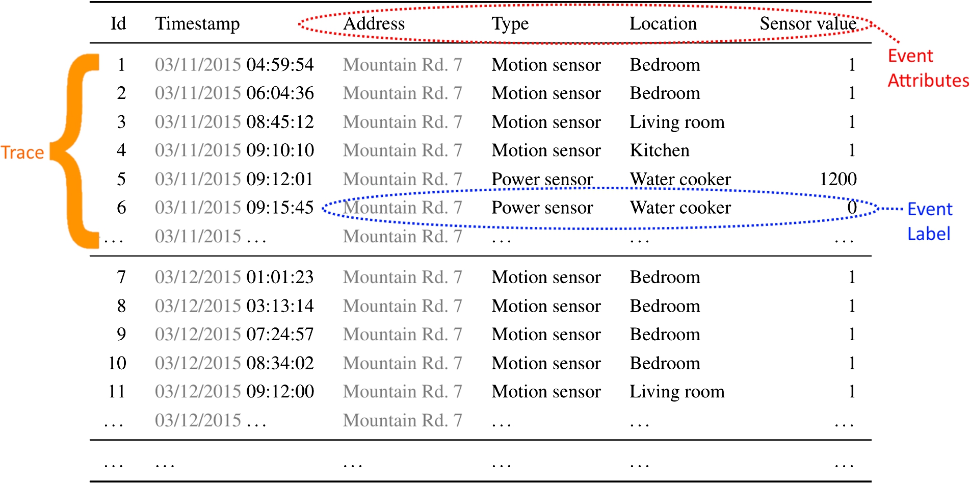
The scope of process mining has broadened in recent years from business process management to other application domains, one of them is the analysis of events of human behavior with data originating from sensors in smart home environments [9,22,38,39,42,43]. Table 1 shows an example of such an event log. Events in the event log are generated by, e.g., motion sensors placed in the house, power sensors placed on appliances, open/close sensors placed on closets and cabinets, etc. Particularly challenging in applying process mining in this application domain is the extraction of meaningful event labels that allow for the discovery of insightful process models. Simply using the sensor that generates an event (the sensor column in Table 1) as event label is shown to produce non-informative process models that overgeneralize the event log and allow for too much behavior [42]. Abstracting sensor-level events into events at the level of human activity (e.g., eating, sleeping, etc.) using activity recognition techniques helps to discover more behaviorally constrained and more insightful process models [43,45]. However, the applicability of this approach relies on the availability of a reliable diary of human behavior at the activity level, which is often expensive or sometimes even impossible to obtain.
Existing approaches that aim at mining temporal relations from smart home environment data [11,18,19,30–32] do not support the rich set of temporal ordering relations that are found in the process models [47], which amongst others include sequential ordering, (exclusive) choice, parallel execution, and loops.
In our earlier work [42], we showed that better process models can be discovered by taking the name of the sensor that generated the event as a starting point for the event label and then refining these event labels using information on the time within the day at which the event occurred. The refinements used in [42] were based on domain knowledge, and not identified automatically from the data. In this paper, we aim at the automatic generation of semantically interpretable label refinements that can be explained to the user, by basing label refinements on data attributes of events. We explore methods to bring parts of the timestamp information to the event label in an intelligent and fully automated way, with the end goal of discovering behaviorally more precise and therefore more insightful process models. Initial work on generating label refinements based on timestamp information was started in [41]. Here, we extend the work started in [41] in two ways. First, we propose strategies to select a set of time-based label refinements from candidate time-based label refinements. Furthermore, add an evaluation of the technique in the form of a case study on a real-life smart home dataset.
We start by introducing basic concepts and notations used in this paper in Section 2. In Section 3, we introduce a framework for the generation of event labels refinements based on the time attribute. In Section 4, we apply this framework on a real-life smart home dataset and show the effect of the refined event labels on process discovery. In Section 5, we address the case of applying multiple label refinements together. We continue by describing related work in Section 6 and conclude in Section 7.
2.Background
In this section, we introduce basic notions related to event logs and relabeling functions for traces and then define the notions of refinements and abstractions. We also introduce some Petri net basics.
We use the usual sequence definition, and denote a sequence by listing its elements, e.g., we write
2.1.Event logs and their components
An event is the most elementary element of an event log. Let
Events are often considered in the context of other events. We call
Often it is useful to partition an event set into smaller sets in which events belong together according to some criterion. We might for example be interested in discovering the typical behavior within a household over the course of a day. In order to do so, we can group together events with the same address and the same day-part of the timestamp (both indicated in gray), as indicated by the horizontal lines in Table 1. For each of these event sets, we can construct a trace; timestamps define the ordering of events within the trace. For events of a trace having the same timestamps, an arbitrary ordering can be chosen within a trace.
Formally, this process of generating traces from an event set is performed based on an event partitioning function, which is a function
An event log L is a finite set of traces
After this relabeling step, some traces of the log can become identically labeled (the event id’s would still be different). The information about the number of occurrences of a sequence of event labels in an event log is highly relevant for process mining, since it allows process discovery algorithms to differentiate between the mainstream behavior of a process (i.e., frequently occurring behavioral patterns) and the exceptional behavior.
Let
An example of an event relabeling function l would be one that relabels events from an event universe
2.2.Process models and process discovery
The goal of process discovery is to discover a process model that represents the behavior seen in an event log. The activities/transitions in this discovered process model describe allowed orderings over the event labels of the events in the event logs. A frequently used process modeling notation in the process mining field is the Petri net notation [29]. Petri nets are directed bipartite graphs consisting of transitions and places, connected by arcs. Transitions represent activities, while places represent the enabling conditions of transitions. Labels are assigned to transitions to indicate the type of activity that they model. A special label τ is used to represent invisible transitions, which are only used for routing purposes and not recorded in the log.
A labeled Petri net
Fig. 1.
An example Petri net.
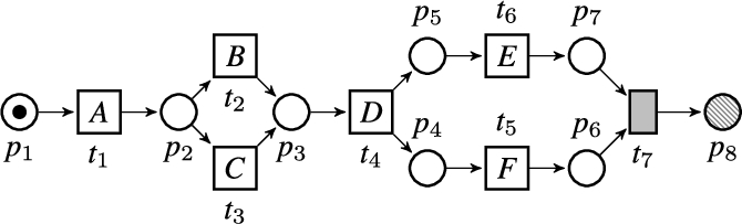
A state of a Petri net is defined by its marking  . Many process modeling notations, including accepting Petri nets, have formal executional semantics and a model defines a language of accepting traces
For an event log L and a process model M we say that L is fitting on process model M if
In process discovery tasks on event logs from the business process management domain, events are often simply relabeled to the value of an activity name attribute, which stores a generally understood name for the event (e.g., receive loan application, or decide on building permit application). However, event logs from the smart home environment domain generally do not contain a single attribute such that relabeling on that attribute enables the discovery of insightful process models [42]. In this paper we explore strategies to refine the event labels that are based on the name of the sensor in a smart home based on information about the time in the day at which the sensor was triggered.
3.A framework for time-based label refinements
In this section, we describe a framework to generate an event label that contains partial information about the event timestamp, in order to make the event labels more specific while preserving interpretability. Note that by bringing time-in-the-day information to the event label we aim at uncovering daily routines of the person under study. We take a clustering-based approach by identifying dense areas in time-space for each event label. The time part of the timestamps consists of values between 00:00:00 and 23:59:59, equivalent to the timestamp attribute from Table 1 with the day-part of the timestamp removed. This timestamp can be transformed into a real number time representation in the interval
Fig. 2.
The histogram representation and a Gaussian Mixture Model fitted to timestamps values of the plates cupboard sensor in the Van Kasteren [50] dataset.
![The histogram representation and a Gaussian Mixture Model fitted to timestamps values of the plates cupboard sensor in the Van Kasteren [50] dataset.](https://content.iospress.com:443/media/ais/2019/11-2/ais-11-2-ais190519/ais-11-ais190519-g004.jpg)
A well-known type of mixture model is the Gaussian Mixture Model (GMM), where the components in the mixture distributions are normal distributions. The data space of time is, however, non-Euclidean: it has a circular nature, e.g., 23.99 is closer to 0 than to 23. This circular nature of the data space introduces problems for GMMs. Figure 2 illustrates the problem of GMMs in combination with circular data by plotting the timestamps of the bedroom sensor events of the Van Kasteren [50] real-life smart home event log. The GMM fitted to the timestamps of the sensor events consists of two components, one with the mean at 9.05 (in red) and one with a mean at 20 (in blue). The histogram representation of the same data shows that some events occurred just after midnight, which on the clock is closer to 20 than to 9.05. The GMM, however, is unaware of the circularity of the clock, which results in a mixture model that seems inappropriate when visually comparing it with the histogram. The standard deviation of the mixture component with a mean at 9.05 is much higher than one would expect based on the histogram as a result of the mixture model trying to explain the data points that occurred just after midnight. The field of circular statistics (also referred to as directional statistics), concerns the analysis of such circular data spaces (cf. [27]). In this paper, we use a mixture of von Mises distributions to capture the daily patterns.
Here, we introduce a framework for generating refinements of event labels based on time attributes using techniques from the field of circular statistics. This framework consists of three stages to apply to the set of timestamps of a sensor:
Data-model pre-fitting stage | A known problem with many clustering techniques is that they return clusters even when the data should not be clustered. In this stage, we assess if the events of a certain sensor should be clustered at all, and if so, how many clusters it contains. For sensor types that are assessed to not be clusterable (i.e., the data consists of one cluster), the procedure ends and the succeeding two stages are not executed. |
Data-model fitting stage | In this stage, we cluster the events of a sensor type by timestamp using a mixture consisting of components that take into account the circularity of the data. The clustering result obtained in the fitting stage is now a candidate label refinement. The event label can be refined based on the clustering result by adding the assigned cluster to the event label, e.g., open/close fridge can be relabeled into three distinct labels open/close fridge 1, open/close fridge 2, and open/close fridge 3 in case the timestamps of the fridge where clustered into three clusters. |
Data-model post-fitting stage | In this stage, the quality of the candidate label refinements is assessed from both a cluster quality perspective and a process model (event ordering statistics) perspective. The event label is only refined when the candidate label refinement is 1) based on a clustering that has a sufficiently good fit with the data, and 2) helps to discover a more insightful process model. If the candidate label refinement does not pass one of the two tests, the label refinement candidate will not be applied (i.e., the event label will remain to only consist of the sensor name). |
In the proceeding sections we describe these three stages in detail.
3.1.Data-model pre-fitting stage
This stage consists of three procedures: a test for uniformity, a test for unimodality, and a method to select the number of clusters in the data. If the timestamps of a sensor type are considered to be uniformly distributed or follow a unimodal distribution, the data is considered not to be clusterable, and the sensor type will not be refined. If the timestamps are neither uniformly distributed nor unimodal, then the procedure for the selection of the number of clusters will decide on the number of clusters used for clustering.
3.1.1.Uniformity check
Rao’s spacing test [34] tests the uniformity of the timestamps of the events from a sensor around the circular clock. This test is based on the idea that uniform circular data is distributed evenly around the circle, and n observations are separated from each other
Given n successive observations
3.1.2.Unimodality check
Hartigan’s dip test [15] tests the null hypothesis that the data follows a unimodal distribution on a circle. When the null hypothesis can be rejected, we know that the distribution of the data is at least bimodal. Hartigan’s dip test measures the maximum difference between the empirical distribution function and the unimodal distribution function that minimizes that maximum difference.
3.1.3.Selecting the number of mixture components
The Bayesian Information Criterion (BIC) [37] introduces a penalty for the number of model parameters to the evaluation of a mixture model. Adding a component to a mixture model increases the number of parameters of the mixture with the number of parameters of the distribution of the added component. The likelihood of the data given the model can only increase by adding extra components, adding the BIC penalty results in a trade-off between the number of components and the likelihood of the data given the mixture model. BIC is formally defined as
3.2.Data-model fitting stage
A generic approach to estimate a probability distribution from data that lies on a circle or any other type of manifold (e.g., the torus and sphere) was proposed by Cohen and Welling in [6]. However, their approach estimates the probability distribution on a manifold in a non-parametric manner, and it does not use multiple probability distribution components, making it unsuitable as a basis for clustering.
We cluster events generated by one sensor using a mixture model consisting of components of the von Mises distribution, which is the circular equivalent of the normal distribution. This technique is based on the approach of Banerjee et al. [3] that introduces a clustering method based on a mixture of von Mises–Fisher distribution components, which is a generalization of the 2-dimensional von Mises distribution to n-dimensional spheres. A probability density function for a von Mises distribution with mean direction μ and concentration parameter κ is defined as
3.3.Data-model post-fitting stage
This stage consists of two procedures: a statistical test to assess how well the clustering result fits the data, and a test to assess whether the ordering relations in the log become stronger by applying the relabeling function (i.e., whether it becomes more likely to discover a precise process model with process discovery techniques).
3.3.1.Goodness-of-fit test
After fitting a mixture of von Mises distributions to the sensor events, we perform a goodness-of-fit test to check whether the data could have been generated from this distribution. We describe the Watson
3.3.2.Control flow test
The clustering obtained can be used as a label refinement where we refine the original event label into a new event label for each cluster. We assess the quality of this label refinement from a process perspective using the label refinement evaluation method described in [42]. This method tests whether the log statistics that are used internally in many process discovery algorithms become significantly more deterministic by applying the label refinement. Hence, we test whether the models become more precise after time-based label refinement. An example of such a log statistic is the direct successor statistic:
Fig. 3.
Process models discovered on the Van Kasteren data with sensor-level event labels (a) and refined event labels (b) with the Inductive Miner infrequent (20% filtering).
4.Case study
We apply our time-based label refinements approach to the real-life smart home dataset described in Van Kasteren et al. [50]. The Van Kasteren dataset consists of 1285 events divided over fourteen different sensors. We segment in days from midnight to midnight to define cases. Note that we consider the data of the Van Kasteren on the sensor level, therefore each event label in the log corresponds to a sensor. Since this dataset originates from the activity recognition field it also contains events at the level of human activities, instead of on the level of sensors. However, we focus on the sensor behavior since we want our analysis methodology to be directly applicable to smart home environments, without the need of first applying activity recognition techniques.
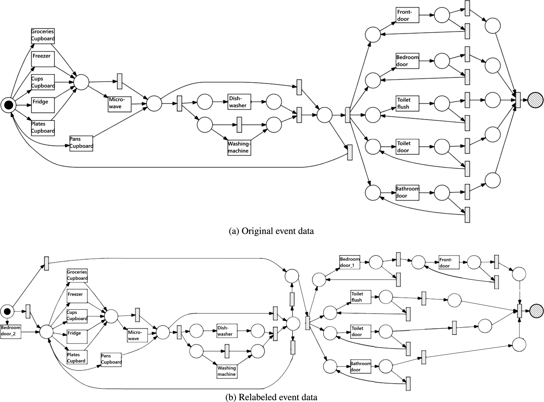
Figure 3(a) shows the process model discovered on this event log with the Inductive Miner infrequent [21] process discovery algorithm with 20% filtering, which is a state-of-the-art process discovery algorithm that discovers a process model that describes the most frequent 80% of behavior in the log. Note that this process model overgeneralizes, i.e., it allows for too much behavior. At the start, a (possibly repeated) choice is made between five transitions. At the end of the process, the model allows any sequence over the alphabet of five activities, where each event label occurs at least once.
We illustrate the framework by applying it to the bedroom door sensor. Rao’s spacing test results in a test statistic of 241.0 with 152.5 being the critical value for significance level 0.01, indicating that we can reject the null hypothesis of a uniformly distributed set of bedroom door timestamps. Hartigan’s dip test results in a p-value of
Fig. 4.
BIC values for different numbers of components in the mixture model.

Table 2
Estimated parameters for a mixture of von Mises components for bedroom door sensor events
| Cluster | α | μ (radii) | κ |
| Cluster 1 | 0.76 | 2.05 | 3.85 |
| Cluster 2 | 0.24 | 5.94 | 1.56 |
Figure 3(b) shows the process model discovered with the Inductive Miner infrequent with 20% filtering after applying this label refinement to the Van Kasteren event log. The process model still overgeneralizes the overall process, but the label refinement does help to restrict the behavior, as it shows that the evening bedroom door events are succeeded by one or more events of type groceries cupboard, freezer, cups cupboard, fridge, plates cupboard, or pans cupboard, while the morning bedroom door events are followed by one or more frontdoor events. It seems that this person generally goes to the bedroom in-between coming home from work and starting to cook. The loop of the frontdoor events could be caused by the person leaving the house in the morning for work, resulting in no logged events until the person comes home again by opening the frontdoor. Note that in Fig. 3(a) bedroom door and frontdoor events can occur an arbitrary number of times in any order. Figure 3(a) furthermore does not allow for the bedroom door to occur before the whole block of kitchen-located events at the beginning of the net.
In the process mining field, multiple quality criteria exist to express the fit between a process model and an event log. Two of those criteria are fitness [36], which measures the degree to which the behavior that is observed in the event log can be replayed on the process model, and precision [28], which measures the degree to which the behavior that was never observed in the event log cannot be replayed on the process model. Low precision typically indicates an overly general process model, that allows for too much behavior. Typically we aim for process models with both high fitness and precision. Therefore, one can consider the harmonic mean of the two, often referred to as F-score. The bedroom door label refinement described above improves the precision of the process model found with the Inductive Miner infrequent (20% filtering) [21] from 0.3577 when applied on the original event log to 0.4447 when applied on the refined event log and improves the F-score from 0.5245 to 0.6156.
Fig. 5.
Inductive Miner infrequent (20% filtering) result after a second label refinement.
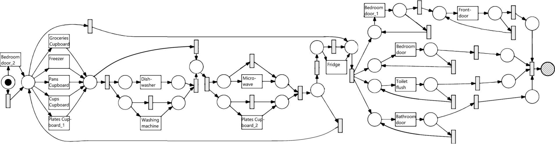
The label refinement framework allows for refinement of multiple activities in the same log. For example, label refinements can be applied iteratively. Figure 5 shows the effect of a second label refinement step, where Plates cupboard using the same methodology is refined into two event labels, representing time ranges [7.98–14.02] and [16.05–0.92] respectively. This refinement shows the additional insight that the evening version of the Plates cupboard occurs directly before or after the microwave. Generating multiple label refinements, however, comes with the problem that the control-flow test [42] is sensitive to the order in which label refinements are applied. Because label refinements change the event log, it is possible that after applying some label refinement A, some other label refinement B starts passing the control-flow test that did not pass this test before, or fails the test while it passed before. Additionally, applying one label refinement can change the information gain of applying another label refinement afterward. For example, when
5.On the ordering of label refinements
As shown in Section 4, the outcome of the control flow test of a label refinement can depend on whether other possible label refinements that have passed the test of the pre-fitting and post-fitting stages have already been applied. Therefore, in this section, we explore on three real-life event logs the effect of the ordering in which label refinements are applied.
5.1.Label refinement selection strategies
To explore the effect of the order in which label refinements are applied, we investigate four strategies to select a set of label refinements to apply to the event log and we evaluate these four strategies on the evaluation logs. Each of the strategies assumes the desired number k of label refinements to be given.
All-at-once | This strategy can be seen as a naive strategy that ignores the influence of interplay between label refinements on the outcome of the control flow test. It simply applies the three stages of the framework to generate label refinements to each of the sensors in the event logs, and out of all the sensors that pass the statistical significance tests it selects the top k sorted on their information gain, i.e. all the information values are calculated using the original event log on which none of the other possible selected label refinements have been applied. |
Exhaustive Search | The exhaustive search strategy takes the effect on the information gain of the order in which label refinements are applied fully into account and finds the optimal set of k label refinements. To achieve this goal, starting from the set of label refinements that have passed the statistical significance tests, the strategy investigates all possible orderings in which these label refinements can be applied to the log and calculates for each ordering of label refinements the total information gain that is achieved with it. To calculate this total information gain, the information gain of each label refinement in this ordering is calculated on the log to which all label refinements earlier in the ordering are already applied. While the label refinement sequence that is found with this strategy is optimal in terms of total information gain, this strategy can quickly become computationally intractable for event logs that contain many sensors. |
Greedy Search | This strategy performs a greedy search. It first applies the best label refinement in terms of information gain on the original log and refines the event log using this label refinement. Then, it iterates to find the next label refinement by calculating the information gain using the refined event log from the previous step. The procedure is continued until k refinements have been found. Note that this strategy leads to a considerably smaller search space compared to the exhaustive search strategy, as at each iteration only the best label refinement is applied and the next iteration continuous only from this best label refinement. |
Beam Search | The beam search strategy at is similar to the greedy search strategy, with the difference that at each iteration it keeps a predetermined number b (called the beam size) of best partial solutions are kept as candidates, while the greedy search only keeps the single best candidate. Only the best b combinations in terms of information gain that were found consisting of n label refinements are explored to search for a new set of |
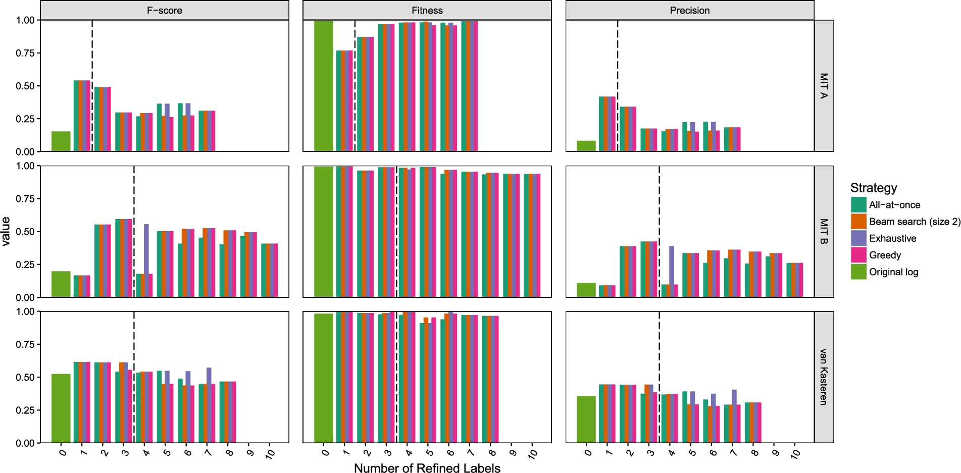
Fig. 6.
Fitness, precision, and F-score of the Inductive Miner infrequent (20% filtering) models obtained from the original and refined versions of three event logs.
5.2.Experimental setup
Label refinements can lead to a decrease in the fitness of the resulting process model, while at the same time increasing its precision. The reason for this is that a very imprecise process model, i.e. one that allows for all behavior, is by definition perfectly fitting. As a result, changing to a process model that makes a more specific, i.e. more precise, description of the behavior can only bring fitness down. To see why refinements can increase precision while fitness can decrease, consider a refinement of a sensor type a into a refined
We apply these four strategies on three event logs from smart home environments and measure the fitness, precision, and F-score of the models that are discovered with the Inductive Miner infrequent [21] with 20% filtering after each label refinement. The first event log is the Van Kasteren [50] event log which we introduced in Section 4. The other two event logs are two different households of a smart home experiment conducted by MIT [40]. The log Household A of the MIT experiment contains 2701 events spread over 16 days, with 26 different sensors. The Household B log contains 1962 events spread over 17 days and 20 different sensors. Note that, like for the Van Kasteren dataset, we consider the events from the MIT A and B datasets on the sensor level instead of on the human activity level. Therefore, the event labels in the log each correspond to a sensor.
The choice between the four strategies can be seen as a trade-off between the degree in which they can take the effect of the ordering of label refinements into account and the computational effort that they require. Note that when the impact of the label refinements that are already applied to the log on the information gain of succeeding label refinements is large, then we expect the exhaustive search strategy to outperform the other strategies. In contrast, in the case that label refinements are mostly mutually independent and there is no strong effect of which label refinements have already been applied to the log on the usefulness in terms of information gain when applying a certain other label refinement, then the all-at-once strategy would suffice to find a set of label refinements and the considerable computational effort needed to perform an exhaustive search would be unnecessary, thereby enabling us to find sets of label refinements for logs with high numbers of sensors. The experiments in which we apply the four search strategies to generate label refinements are intended to investigate the degree to which the order of label refinements matter, i.e., the degree to which one label refinement impacts the usefulness of other label refinements.
5.3.Results
Figure 6 shows the fitness, precision, and F-score values of the process models that were discovered after selecting label refinements with each of the four strategies on the three event logs. The precision can be improved considerably through label refinements on all three event logs.
While the fitness decreased on the MIT A log as an effect of the refinements, fitness is not so much affected by refining the labels on the MIT B and the Van Kasteren event logs. The reason for this is that is when the relation between sensors that is exposed by the label refinement holds in almost all cases, there is almost no loss in fitness, i.e., if 100% of the
Note that all strategies find the exact same label refinement as first label refinement, since with only one label refinement there is no notion of interplay between label refinements. When refining a second event label the four strategies all select the same label refinement on all three logs, hinting that in practice the effect of interplay between label refinements is not very strong. Since all four strategies selected the same second label refinement, the F-score, fitness, and precision are also identical for the four strategies. Figure 6 shows that for the MIT household A data set there are 7 sensor types that can be refined, i.e., they passed the statistical tests of the pre-fitting stage and their obtained clustering passed the goodness-of-fit test. For the MIT household B data set there are 10 sensor types that can be refined and there are 8 sensor types that can be refined for the Van Kasteren data set. However, since the F-score for all strategies drops again after a few label refinements, not all of those label refinements lead to better process models. The four strategies perform very similar in terms of F-score.
Exhaustive search outperforms the other strategies for a few refinements on some logs, however, such improvements come with considerable computation times. On the MIT household B log, which has 10 possible label refinements, it takes about 25 minutes on an Intel i7 processor to evaluate all possible combinations of refinements. On logs with even more possible refinements the exhaustive strategy can quickly become computationally infeasible. The computational complexity of the exhaustive strategy stems from the fact that the ordering in which label refinements are applied can influence their information gain, and therefore the set of candidate label refinement sequences to consider is equal to the number of permutations on the number of activities (i.e.
The all-at-once strategy is computationally very fast and only takes milliseconds to compute on all event logs. Note that with this strategy the information gain only needs to be calculated once for every event label in the log, therefore the computational complexity is
Since the F-score decreases again when applying too many label refinements it is important to have a stopping criterion that prevents refining the event log too much. The dashed line in Fig. 6 shows the results when we only refine a label when the information gain of the refinement is larger than zero. On the MIT households A and B logs this stopping criterion causes all strategies to stop at the best combination of label refinements in F-score, consists respectively of one and three refinements. This indicates that the control flow test [42] provides a useful stopping criterion for label refinements.
As the greedy search strategy iteratively selects the best label refinement, its computational complexity is
All strategies except the exhaustive search strategy suggest as the fourth refinement for MIT B a refinement that decreases the F-score sharply, to increase it again with a fifth refinement. This is caused by an unhelpful refinement being found as the fourth refinement by those strategies, which causes the frequencies to drop below the filtering threshold of the Inductive Miner, leading to a model that is less precise. At the fifth refinement, the follows statistics of other activities drop as well, causing the follows statistics that dropped in the fourth refinement to be relatively higher and above the threshold again. On the Van Kasteren log the optimum in F-score is to make only one refinement, although the F-score after applying the second and third refinement as found by the exhaustive and beam search is almost identical. The all-at-once strategy stops after applying only two refinements while the other strategies apply a third refinement. The best refinement combination found with the all-at-once strategy using the stopping criterion is identical to the refinement combination found with the other strategies, suggesting that in practice the differences between the four approaches are small. On real-life smart home environment event logs the effect that one label refinement influences the control flow test outcome of others is limited.
Fig. 7.
The Inductive Miner infrequent (20% filtering) process model discovered from the original MIT a event log.
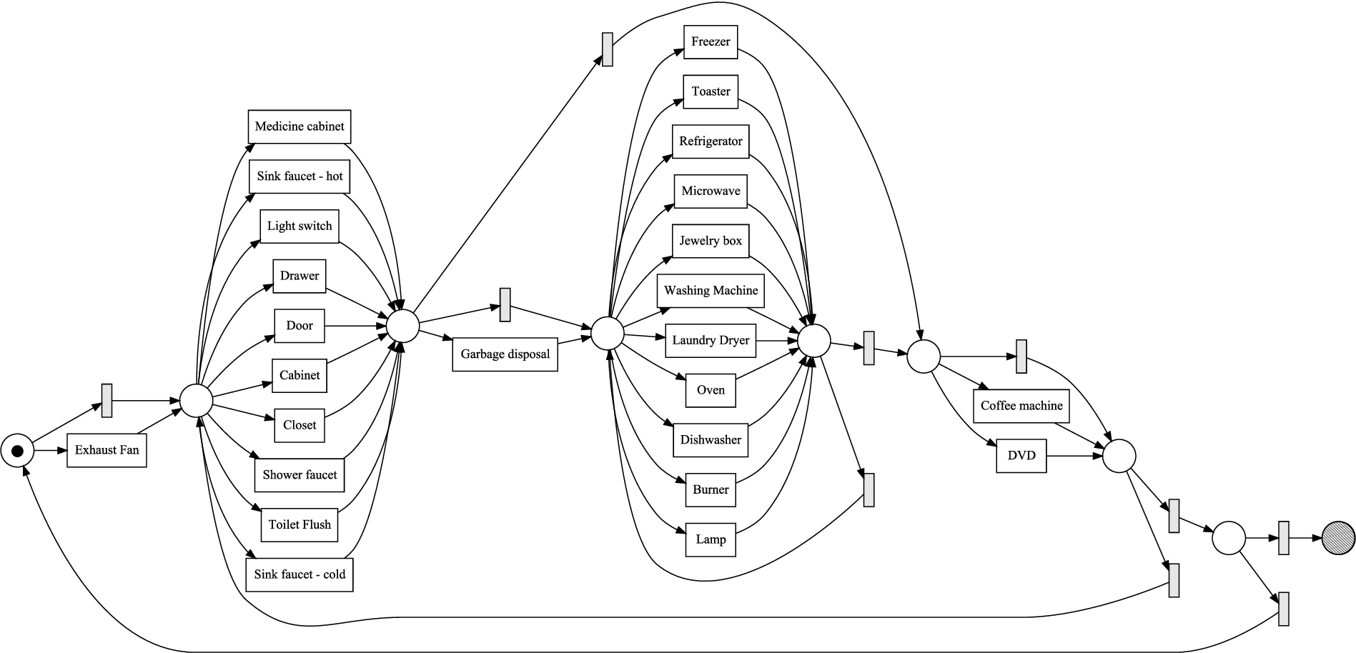
Fig. 8.
The Inductive Miner infrequent (20% filtering) process model discovered from the refined MIT A event log.
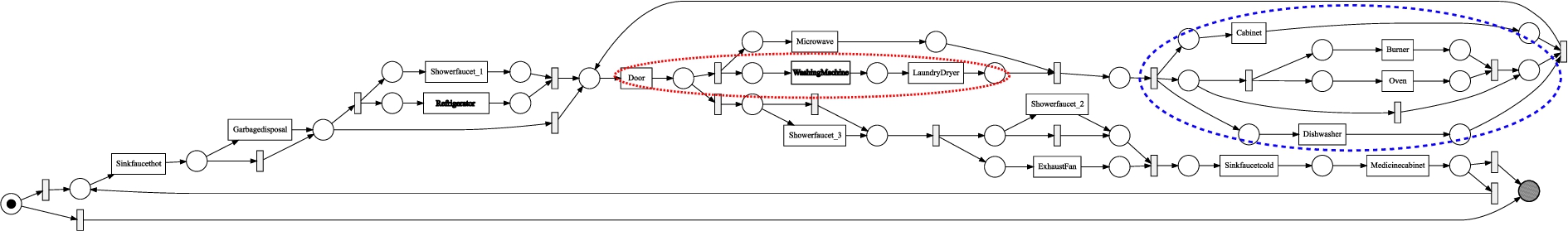
Figures 7 and 8 shows the process model that are discovered with the Inductive Miner infrequent with 20% filtering respectively from the original MIT household A event log and the event log obtained after applying the optimal combination of label refinements found in the results of Fig. 6. Because of the silent transitions, the process model discovered from the original event log allows for almost all orderings over the sensor types. Even though the transition labels in the process model discovered from the refined event log are not readable because of the size, it is clear from the structure of the process model that it is much more behaviorally specific, containing a mix of sequential orderings, parallel blocks, and choices over the sensor types. Especially interesting is the part indicated by the blue dashed ellipse, which contains a parallel block consisting of a cabinet, the oven and burner, and the dishwasher, showing a clearly recognizable cooking routine. Furthermore, the part indicated by the red dotted ellipse indicates a sequentially ordered part, consisting of some door sensor registering the opening of a door, followed by starting the washing machine and then the laundry dryer.
The time-based label refinement generation framework as well as the four strategies to generate multiple label refinements on the same event log are implemented and publicly available in the process mining toolkit ProM [49] as part of the LabelRefinements11 package.
6.Related work
We classify related work into three categories. The first category of related work concerns techniques from the process mining field, specifically focusing on techniques that, like our approach, focus on refining event labels. The second category of related work, also originating from the process mining area, focuses on the interplay between ordering between process activities and external information, such as time. The third category of related work originates from the ambient intelligence and smart home environments field, focusing on work on mining temporal relations between human activities. We use these three categories to structure this section.
6.1.Label splits and refinements in process mining
The task of finding refinements of event labels in the event log is closely related to the task of mining process models with duplicate activities, in which the resulting process model can contain multiple transitions/nodes with the same label. From the point of view of the behavior that is allowed by a process model, it makes no difference whether a process model is discovered on an event log with refined event labels, or whether a process model is discovered with duplicate activities such that each transition/node of the duplicate activity precisely covers one version of the refined event label. However, a refined event label may also provide additional insights as the new event labels are explainable in terms of time. The first process discovery algorithm capable of discovering duplicate tasks was proposed by Herbst and Karagiannis in 2004 [16], after which many others have been proposed, including the Evolutionary Tree Miner [5], the
The work that is closest to our work is the work by Lu et al. [26], who describe an approach to pre-process an event log by refining event labels with the goal of discovering a process model with duplicate activities. The method proposed by Lu et al., however, does not base the relabelings on data attributes of those events and only uses the control flow context, leaving uncertainty whether two events relabeled differently are actually semantically different.
6.2.Data-aware process mining
Another area of related work is data-aware process mining, where the aim is to discover rules with regard to data attributes of events that decide decision points in the process. De Leoni and van der Aalst [7] proposed a method that discovers data guards for decision points in the process based on alignments and decision tree learning. This approach relies on the discovery of a behaviorally well-fitting process model from the original event log. When only overgeneralizing process models (i.e., allowing for too much behavior) can be discovered from an event log, the correct decision points might not be present in the discovered process model at all, resulting in this approach not being able to discover the data dependencies that are in the event log. Our label refinements use data attributes prior to process discovery to enable the discovery of more behaviorally constrained process models by bringing parts of the event attribute space to the event label.
6.3.Temporal relation mining for smart home environments
Galushka et al. [11] provide an overview of temporal data mining techniques and discuss their applicability to data from smart home environments. Many of the techniques described in the overview focus on real-valued time series data, instead of discrete sequences which we assume as input in this work. For discrete sequence data, Galushka et al. [11] propose the use of sequential rule mining techniques, which can discover rules of the form “if event a occurs then event b occurs with time T”.
Huynh et al. [18] proposed to use topic modeling to mine activity patterns from sequences of human events. Topic modeling originates from the field of natural language processing and addresses the challenge to find topics in textual documents and assign a distribution over these topics to each document. However, the discovered topics do not represent the human activities in terms of control-flow ordering constructs like sequential ordering, concurrent execution, choices, and loops.
Ogale et al. [31] proposed an approach to describe the temporal relation between human behavior activities from video data using context-free grammars, using the human poses extracted from the video as the alphabet. Like Petri nets, context-free grammars define a formal language over its alphabet. However, Petri nets have a graphical representation, which is lacking for grammars. Furthermore, as shown by Peterson [32], Petri net languages are a subclass of context-sensitive languages, and some Petri net languages are not context-free. This indicates that some relations over activities that can be expressed in Petri nets cannot be expressed in a context-free grammar.
One particularly related technique, called TEmporal RElation Discovery of Daily Activities (TEREDA), was proposed by Nazerfard et al. [30]. TEREDA leverages temporal association rule mining techniques to mine ordering relations between activities as well as patterns in their timestamp and duration. The ordering relations between activities that are discovered by TEREDA are restricted to the form “activity a follows activity b”, where our proposed approach of modeling the relations with Petri nets allow for modeling of more complex relations between larger number of activities, such as: “the occurrences of activity b that are preceded by activity a are followed by both activity d and e, but in arbitrary order”. The patterns in the timestamps are obtained by fitting a Gaussian Mixture Model (GMM) with the Expectation–Maximization (EM) algorithm, thereby ignoring problems caused by the circularity of the 24-hour clock introduced in this paper.
Jukkala and Cook [19] propose a method to mine temporal relations between activities from smart home environments logs where the temporal relation patterns are expressed in Allen’s interval algebra [1]. Allen’s interval algebra allows the expression of thirteen distinct types of temporal relations between two activities based on both the start and end timestamps of these activities. The approach of Jukkala and Cook [19] is limited to describing the relations between pairs of activities, and more complex relations between three or higher numbers of activities cannot be discovered. The aim of mining the patterns in Allen’s interval algebra representation is to increase the accuracy of activity recognition systems, while our goal is knowledge discovery. Several papers from the process mining area have focused on mining temporal relations between activities from smart home event logs. Leotta et al. [22] postulate three main research challenges for the applicability of process mining technique for smart home data. One of those three challenges is to improve process mining techniques to address the less structured nature of human behavior as compared to business processes. Our technique addresses this challenge, as the time-based label refinements help in uncovering relations between activities with process mining techniques that could not be found without applying time-based label refinements.
DiMaggio et al. [9] and Sztyler et al. [38,39] propose to mine Fuzzy Models [14] to describe the temporal relations between human activities. The Fuzzy Miner [14], a process discovery algorithm that mines a Fuzzy Model from an event log, is a process discovery algorithm that is designed specifically for weakly structured processes. However, Fuzzy Models, in contrast to Petri nets, do not define a formal language over the activities, and are therefore not precise on what activity orderings are allowed and which are not. While mining a Fuzzy Model description of human activities is less challenging compared to mining a process model with formal semantics, it is also limited in the insights that can be obtained from it.
Finally, insights in the human routines can be obtained through the discovery of Local Process Models [44], which bridges process mining and sequential pattern mining by finding patterns that include high-level process model constructs such as (exclusive) choices, loops, and concurrency. However, Local Process Models, as opposed to process discovery, only give insight into frequent subroutines of behavior and do not provide the global picture of the behavior throughout the day from start to end.
7.Conclusion and future work
We have proposed a framework based on techniques from the field of circular statistics to refine event labels automatically based on their timestamp attribute. We have shown on a real-life event log that this framework can be used to discover label refinements that allow for the discovery of more insightful and behaviorally more specific process models. Additionally, we explored four strategies to search combinations of label refinements. We found that the difference between an all-at-once strategy, which ignores that one label refinement can have an effect on the usefulness of other label refinements, and other more computationally expensive strategies is often limited. As a result of this finding, the fast but approximate label refinement strategies can in practice be applied instead of performing a full exhaustive search, thereby enabling label refinement search on smart home logs with high numbers of sensors.
An interesting area of future work is to explore the use of other types of event data attributes to refine event labels, e.g., power values of sensors. A next research step would be to explore label refinements based on a combination of data attributes combined. This introduces new challenges, such as the clustering on partially circular and partially Euclidean data spaces. Additionally, other time-based types of circles than the daily circle described in this paper, such as the week, month, or year circle, are worth investigating.
References
[1] | J.F. Allen, Maintaining knowledge about temporal intervals, Communications of the ACM 26: (11) ((1983) ), 832–843. doi:10.1145/182.358434. |
[2] | A. Augusto, R. Conforti, M. Dumas, M. La Rosa and G. Bruno, Automated discovery of structured process models: Discover structured vs. discover and structure, in: Proceedings of the International Conference on Conceptual Modeling, Springer, (2016) , pp. 313–329. doi:10.1007/978-3-319-46397-1_25. |
[3] | A. Banerjee, I.S. Dhillon, J. Ghosh and S. Sra, Clustering on the unit hypersphere using von Mises–Fisher distributions, Journal of Machine Learning Research 6: ((2005) ), 1345–1382. |
[4] | T. Benaglia, D. Chauveau, D. Hunter and D. Young, Mixtools: An R package for analyzing finite mixture models, Journal of Statistical Software 32: (6) ((2009) ), 1–29. doi:10.18637/jss.v032.i06. |
[5] | J.C.A.M. Buijs, B.F. van Dongen and W.M.P. van der Aalst, On the role of fitness, precision, generalization and simplicity in process discovery, in: OTM Confederated International Conferences “On the Move to Meaningful Internet Systems”, Springer, (2012) , pp. 305–322. |
[6] | T. Cohen and M. Welling, Harmonic exponential families on manifolds, in: Proceedings of the 32nd International Conference on Machine Learning, JMLR W&CP, (2015) , pp. 1757–1765. |
[7] | M. de Leoni and W.M.P. van der Aalst, Data-aware process mining: Discovering decisions in processes using alignments, in: Proceedings of the 28th Annual ACM Symposium on Applied Computing, ACM, (2013) , pp. 1454–1461. |
[8] | A.P. Dempster, N.M. Laird and D.B. Rubin, Maximum likelihood from incomplete data via the EM algorithm, Journal of the Royal Statistical Society. Series B. ((1977) ), 1–38. |
[9] | M. Dimaggio, F. Leotta, M. Mecella and D. Sora, Process-based habit mining: Experiments and techniques, in: Proceedings of the IEEE International Conference on Ubiquitous Intelligence & Computing, IEEE, (2016) , pp. 145–152. |
[10] | F. Folino, G. Greco, A. Guzzo and L. Pontieri, Discovering expressive process models from noised log data, in: Proceedings of the International Database Engineering & Applications Symposium, ACM, (2009) , pp. 162–172. |
[11] | M. Galushka, D. Patterson and N. Rooney, Temporal data mining for smart homes, in: Designing Smart Homes, Springer, (2006) , pp. 85–108. doi:10.1007/11788485_6. |
[12] | S. Goedertier, D. Martens, J. Vanthienen and B. Baesens, Robust process discovery with artificial negative events, Journal of Machine Learning Research 10: (Jun) ((2009) ), 1305–1340. |
[13] | C.-Q. Gu, H.-Y. Chang and Y. Yi, Workflow mining: Extending the α-algorithm to mine duplicate tasks, in: Proceedings of the International Conference on Machine Learning and Cybernetics, Vol. 1: , IEEE, (2008) , pp. 361–368. |
[14] | C. Günther and W.M.P. van der Aalst, Fuzzy mining–adaptive process simplification based on multi-perspective metrics, in: Proceedings of the International Conference on Business Process Management, Springer, (2007) , pp. 328–343. doi:10.1007/978-3-540-75183-0_24. |
[15] | J.A. Hartigan and P.M. Hartigan, The dip test of unimodality, The Annals of Statistics ((1985) ), 70–84. |
[16] | J. Herbst and D. Karagiannis, Workflow mining with InWoLvE, Computers in Industry 53: (3) ((2004) ), 245–264. doi:10.1016/j.compind.2003.10.002. |
[17] | K. Hornik and B. Grün, movMF: An R package for fitting mixtures of von Mises–Fisher distributions, Journal of Statistical Software 58: (10) ((2014) ), 1–31. doi:10.18637/jss.v058.i10. |
[18] | T. Huynh, M. Fritz and B. Schiele, Discovery of activity patterns using topic models, in: Proceedings of the 10th International Conference on Ubiquitous Computing, ACM, (2008) , pp. 10–19. |
[19] | V.R. Jakkula and D.J. Cook, Using temporal relations in smart environment data for activity prediction, in: Proceedings of the ICML Workshop on the Induction of Process Models, (2007) . |
[20] | R.E. Kass and A.E. Raftery, Bayes factors, Journal of the American Statistical Association 90: (430) ((1995) ), 773–795. doi:10.1080/01621459.1995.10476572. |
[21] | S.J.J. Leemans, D. Fahland and W.M.P. van der Aalst, Discovering block-structured process models from event logs containing infrequent behaviour, in: Proceedings of the International Conference on Business Process Management, Springer, (2013) , pp. 66–78. |
[22] | F. Leotta, M. Mecella and J. Mendling, Applying process mining to smart spaces: Perspectives and research challenges, in: Enterprise, Business-Process and Information Systems Modeling, Springer, (2015) , pp. 298–304. |
[23] | J. Li, D. Liu and B. Yang, Process mining: Extending α-algorithm to mine duplicate tasks in process logs, in: Advances in Web and Network Technologies, and Information Management, Springer, (2007) , pp. 396–407. doi:10.1007/978-3-540-72909-9_43. |
[24] | V. Liesaputra, S. Yongchareon and S. Chaisiri, Efficient process model discovery using maximal pattern mining, in: Proceedings of the International Conference on Business Process Management, Springer, (2015) , pp. 441–456. doi:10.1007/978-3-319-23063-4_29. |
[25] | K. Liu, W.K. Cheung and J. Liu, Extracting behavioral motifs for characterizing human daily activities in smart environments, in: Proceedings of the ACM SIGKDD Workshop on Health Informatics, (2012) , pp. 1–8. |
[26] | X. Lu, D. Fahland, F.J.H.M. van den Biggelaar and W.M.P. van der Aalst, Handling duplicated tasks in process discovery by refining event labels, in: Proceedings of the International Conference on Business Process Management, Springer, (2016) , pp. 90–107. doi:10.1007/978-3-319-45348-4_6. |
[27] | K.V. Mardia and P.E. Jupp, Directional Statistics, Vol. 494: , John Wiley & Sons, (2009) . |
[28] | J. Munoz-Gama and J. Carmona, A fresh look at precision in process conformance, in: Proceedings of the International Conference on Business Process Management, Springer, (2010) , pp. 211–226. doi:10.1007/978-3-642-15618-2_16. |
[29] | T. Murata, Petri nets: Properties, analysis and applications, Proceedings of the IEEE 77: (4) ((1989) ), 541–580. doi:10.1109/5.24143. |
[30] | E. Nazerfard, P. Rashidi and D. Cook, Using association rule mining to discover temporal relations of daily activities, Toward Useful Services for Elderly and People with Disabilities ((2011) ), 49–56. |
[31] | A. Ogale, A. Karapurkar and Y. Aloimonos, View-invariant modeling and recognition of human actions using grammars, Springer, (2007) , pp. 115–126. |
[32] | J.L. Peterson, Petri Net Theory and the Modeling of Systems, Prentice Hall, (1981) . |
[33] | R Core Team, R: A Language and Environment for Statistical Computing, R Foundation for Statistical Computing, Vienna, Austria, (2013) , ISBN 3-900051-07-0. http://www.R-project.org/. |
[34] | J. Rao, Some tests based on arc-lengths for the circle, Sankhyā: The Indian Journal of Statistics, Series B ((1976) ), 329–338. |
[35] | W. Reisig and G. Rozenberg, Lectures on Petri Nets I: Basic Models: Advances in Petri Nets, Vol. 1491: , Springer Science & Business Media, (1998) . doi:10.1007/3-540-65306-6. |
[36] | A. Rozinat and W.M.P. van der Aalst, Conformance checking of processes based on monitoring real behavior, Information Systems 33: (1) ((2008) ), 64–95. doi:10.1016/j.is.2007.07.001. |
[37] | G. Schwarz, Estimating the dimension of a model, The Annals of Statistics 6: (2) ((1978) ), 461–464. doi:10.1214/aos/1176344136. |
[38] | T. Sztyler, J. Carmona, J. Völker and H. Stuckenschmidt, Self-tracking reloaded: Applying process mining to personalized health care from labeled sensor data, in: Transactions on Petri Nets and Other Models of Concurrency XI, Springer, (2016) , pp. 160–180. doi:10.1007/978-3-662-53401-4_8. |
[39] | T. Sztyler, J. Völker, J. Carmona, O. Meier and H. Stuckenschmidt, Discovery of personal processes from labeled sensor data – an application of process mining to personalized health care, in: Proceedings of the International Workshop on Algorithms & Theories for the Analysis of Event Data, CEUR-ws.org, (2015) , pp. 22–23. |
[40] | E.M. Tapia, S.S. Intille and K. Larson, Activity recognition in the home using simple and ubiquitous sensors, in: Proceedings of the International Conference on Pervasive Computing, Springer, (2004) , pp. 158–175. |
[41] | N. Tax, E. Alasgarov, N. Sidorova and R. Haakma, On generation of time-based label refinements, in: Proceedings of the 25th International Workshop on Concurrency, Specification and Programming, (2016) . |
[42] | N. Tax, N. Sidorova, R. Haakma and W.M.P. van der Aalst, Log-based evaluation of label splits for process models, Procedia Computer Science 96: ((2016) ), 63–72. doi:10.1016/j.procs.2016.08.096. |
[43] | N. Tax, N. Sidorova, R. Haakma and W.M.P. van der Aalst, Event abstraction for process mining using supervised learning techniques, in: Proceedings of the SAI Conference on Intelligent Systems, Springer, (2016) , pp. 161–170. |
[44] | N. Tax, N. Sidorova, R. Haakma and W.M.P. van der Aalst, Mining local process models, Journal of Innovation in Digital Ecosystems 3: (2) ((2016) ), 183–196. doi:10.1016/j.jides.2016.11.001. |
[45] | N. Tax, N. Sidorova, R. Haakma and W.M.P. van der Aalst, Mining process model descriptions of daily life through event abstraction, in: Intelligent Systems and Applications, Springer, (2018) , Chap. To Appear. |
[46] | W.M.P. van der Aalst, Process Mining: Data Science in Action, Springer Science & Business Media, (2016) . |
[47] | W.M.P. van Der Aalst, A.H.M. Ter Hofstede, B. Kiepuszewski and A.P. Barros, Workflow patterns, Distributed and parallel databases 14: (1) ((2003) ), 5–51. doi:10.1023/A:1022883727209. |
[48] | J.M.E.M. van der Werf, B.F. van Dongen, C.A.J. Hurkens and A. Serebrenik, Process discovery using integer linear programming, Fundamenta Informaticae 94: (3–4) ((2009) ), 387–412. |
[49] | B.F. van Dongen, A.J.M.M. Weijters and W.M.P. van der Aalst, The ProM framework: A new era in process mining tool support, Applications and Theory of Petri Nets ((2005) ), 444. |
[50] | T. van Kasteren, A. Noulas, G. Englebienne and B. Kröse, Accurate activity recognition in a home setting, in: Proceedings of the 10th International Conference on Ubiquitous Computing, ACM, (2008) , pp. 1–9. |
[51] | B. Vázquez-Barreiros, M. Mucientes and M. Lama, Mining duplicate tasks from discovered processes, in: Proceedings of the International Workshop on Algorithms & Theories for the Analysis of Event Data, CEUR-ws.org, (2015) , pp. 78–82. |
[52] | G.S. Watson, Goodness-of-fit tests on a circle. II, Biometrika 49: (1/2) ((1962) ), 57–63. doi:10.1093/biomet/49.1-2.57. |
[53] | A. Weijters and J. Ribeiro, Flexible heuristics miner (FHM), in: Proceedings of the IEEE Symposium on Computational Intelligence and Data Mining (CIDM), IEEE, (2011) , pp. 310–317. |


