
A New Tool for the Analysis of the Effect of Intracerebrally Injected Anti-Amyloid-β Compounds
Abstract
Background:
A wide range of techniques has been developed over the past decades to characterize amyloid-β (Aβ) pathology in mice. Until now, no method has been established to quantify spatial changes in Aβ plaque deposition due to targeted delivery of substances using ALZET® pumps.
Objective:
Development of a methodology to quantify the local distribution of Aβ plaques after intracerebral infusion of compounds.
Methods:
We have developed a toolbox to quantify Aβ plaques in relation to intracerebral injection channels using Zeiss AxioVision® and Microsoft Excel® software. For the proof of concept, intracerebral stereotactic surgery was performed in 50-day-old APP-transgenic mice injected with PBS. At the age of 100 days, brains were collected for immunhistological analysis.
Results:
The toolbox can be used to analyze and evaluate Aβ plaques (number, size, and coverage) in specific brain areas based on their location relative to the point of the injection or the injection channel. The tool provides classification of Aβ plaques in pre-defined distance groups using two different approaches.
Conclusion:
This new analytic toolbox facilitates the analysis of long-term continuous intracerebral experimental compound infusions using ALZET® pumps. This method generates reliable data for Aβ deposition characterization in relation to the distribution of experimental compounds.
INTRODUCTION
Alzheimer’s disease (AD) is a yet incurable neurodegenerative disease and the most common type of dementia in the aging population, affecting approximately 56 million people worldwide [1, 2]. AD is characterized by time- and location-specific accumulation of amyloid-β (Aβ) and hyperphosphorylated tau protein, and inflammatory changes including microglia and astrocyte activation. These morphologic changes lead to synaptic dysfunction and irreversible cognitive impairment, which interfere with the person’s ability to work or complete daily activities [3, 4]. The most prominent neuropathological hallmark of AD are senile plaques that consist of toxic Aβ peptides [5, 6]. Therefore, it is critically important for preclinical research to have a reliable and accurate technique to visualize, identify, characterize, and quantify Aβ aggregates [7].
A wide range of techniques has been applied over the past decades to characterize Aβ pathology in brain tissue. These techniques include microscopic methods that enable visualization and structural determination, separation techniques to analyze and obtain Aβ species of certain sizes, spectroscopic techniques to follow the aggregation process and determine protein shape, and immunology-based methods for quantification of Aβ aggregates [8–13]. Currently, different microscopic techniques are commonly used in combination with immunostaining to collect data of Aβ aggregates including size, shape, location, and density [13]. However, processing of high-resolution, large images requires digital imaging software. Various imaging software tools for microscopy offer a unique range of additional options, for instance, writing semi-automated analytic scripts. With these self-programmed scripts, it is possible to extend the analytic capabilities of the tools, and to obtain custom analyses for specific analytical values. These values can be used to evaluate new therapeutic approaches.
Long-term continuous intracerebral infusion of test substances by using mini-osmotic pumps is an interesting approach in neurodegenerative disease research [14–16]. Mini-osmotic pumps are miniaturized infusion systems that provide consistent and precise drug-delivery to specific sites with variable durations and controlled infusion rates. This technique allows researchers to overcome problems of drug-delivery across physiological barriers such as the blood-brain barrier (BBB) [17]. The miniaturized infusion sets consist of two main parts: a mini-osmotic pump and a brain infusion kit that contains the brain infusion cannula, catheter tube, and depth adjustment spacers. The mini-osmotic pumps are able to deliver the agents for variable durations (from 1 day to 6 weeks) with controlled rates (between 0.11 and 10μl/h). The operation of mini-osmotic pumps, e.g., manufactured by ALZET, is based on the salt layer compartment and the tissue environment in which the pump is implanted. The high osmolality of the salt layer causes water influx from the tissue trough a semipermeable membrane [18].
Our previous study using ALZET® mini-osmotic pumps has shown that inappropriate fixation of the ALZET cannula in a long-term continuous infusion experiment can harm the mouse brain. Therefore, we developed an improved methodology, which provides better stability of the ALZET cannula [19]. Until now, there is no method available how to examine the spatial distribution of Aβ and thus, indirectly also the distribution of the test substances in the brain after local infusion with mini-osmotic pumps. To this end, we present a novel and experimentally validated method for quantification of Aβ plaques after long-term intracerebral brain infusion using mini-osmotic pumps.
Here, we present a custom method to quantify plaques based on their distance from a defined injection point or injection channel using the AxioVision viewer software (Carl Zeiss Vision GmbH) and Excel (Microsoft). We provide all scripts and templates in Supplementary Material 2 and include detailed instructions on how to use these, making the toolbox easily usable also for inexperienced users.
Briefly, we use AxioVision to obtain raw data about plaques and several reference points within the digital slides including the hemispheric borders and the injection channels. In Excel, the data points are processed further, and additional values are calculated. The results are displayed in several customized charts and a schematic visualization of detected plaques can be generated for each slide.
MATERIALS AND METHODS
Preparations
Additional methods (animals, mini-osmotic pumps and surgical techniques, tissue harvesting, and statistical analyses) are provided in Supplementary Material 1.
Immunohistochemical staining and digitization
Paraformaldehyde-fixed brains were embedded in paraffin and cut in 4μm thick coronal sections. Sections for Aβ staining were pre-treated for 5 min with 98%formic acid before being stained with primary antibody anti-human Aβ clone 4G8 (1 : 4,000, BioLegend, USA) using a fully automated immunostaining system BOND-III (Leica Biosystems GmbH, Germany). All incubations with primary antibodies were followed by the development with ‘Bond Polymer Refine Detection’ kit (DS9800, Leica Biosystems GmbH, Germany). After staining, tissue sections were digitized at 230 nm resolution using a Pannoramic MIDI II slide scanner (3DHistotech, Budapest, Hungary).
Required software
Carl Zeiss Vision AxioVision® Viewer
We used the AxioVision viewer V4.8.1.0 (Carl Zeiss Vision GmbH, Germany) with the add-in “Mirax2AxioVision Converter Utility” (further referred to as “M2AV”, Carl Zeiss Vision GmbH, Germany) to obtain raw data about plaques. The add-in “M2AV” has to be installed separately. Note that this add-in is a pre-release software.
We provide our custom script in Supplementary Material 2. To install it, copy the files to the “Carl Zeiss” folder (usually located under “C:∖Users∖Public∖Documents∖Carl Zeiss∖”. It can then be called by selecting the script from the menu “Commander” and submenu “Scripts”.
After all components have been installed, the AxioVision Script Editor found in the menu “Commander” can be used to edit the provided script. This is necessary, as certain folder locations are hardcoded into the script and need to be customized. Set the desired output folder path by changing “Folder” in steps 26, 27, and 55–60 (all steps named “Save Datatable As . . . ” or “Save Image As . . . ”). AxioVision will later export all raw data to the selected folder.
Microsoft Excel
We developed our tool using Microsoft Excel 2016. An automatic compatibility check suggests that the template may work in earlier versions (starting with Excel 2013) with the current Power Query add-in, but we have not tested accurate functionality beyond Excel 2016.
Acquiring raw data (AxioVision)
The M2AV-script “Abeta Pump Animals” uses several built-in commands for automated measurements, image enhancement, object segmentation, binary image clean up, object separation editing of the measurement mask, selection of measurement parameters, definition of measurement frame, measurement of geometric and densitometric features, documentation of measured objects and data storage by saving of measurement data in an Excel-compatible file format (CSV).
The following systematic protocol describes in detail how to use the script in AxioVision. It explains how to import images, how to apply slide-specific settings, and how to quantify Aβ plaques. After finishing these steps, the user will obtain raw data that is required to proceed with the analysis in Excel.
1. Load the image (scanned slide) into AxioVision. Since AxioVision does not support the MRXS file format natively, use the add-in “M2AV”. (This protocol does not cover the use of M2AV. Please refer to the M2AV-manual for further information.)
2. Start the script “Abeta Pump Animals”. This script will guide you through the whole process and show relevant information for each step. Complete and confirm each step to proceed with the next one.
3. Enter a unique slide name (e.g., “BlockID_SlideNo”). This name will be used to identify all data from this slide in later steps in Excel. Note: When importing the data to Excel (Section 4), the underscore will be used to split the slide title. If you want to follow another naming convention, you need to edit the PowerQuery in the PowerQueryEditor.
4. Select the region of interest (ROI) by using the option “draw annotation” (Fig. 1). Carefully outline the entire area that you want to analyze further. The area should contain equal parts from the ipsilateral and the contralateral hemisphere. Do not include any area that does not contain tissue. After finishing the outline, any point can be edited to improve the outline before proceeding to the next step. Important: Note the ipsilateral side for each slide, i.e., does the left or the right hemisphere contain the injection channel. This information will be needed later on when processing the data in Excel (Section 4).
5. Define the hemisphere border by marking two points as seen in Fig. 2. First, mark the upper point where both hemispheres meet. Second, mark the lower point where both hemispheres meet. Use the circle tool. Note: Only the coordinates of the center will be used for further calculations, the size of the circle is irrelevant.
6. Define the injection point and a corresponding point in the contralateral hemisphere as seen in Fig. 3. First, mark the end of the injection needle. Second, mark a corresponding contralateral point. Similar to the previous step, the circle tool and center coordinates are used.
7. Next, AxioVision automatically detects all plaques within the selected ROI. When two plaques are located closely together, AxioVision may recognize them wrongly as a single plaque. You have to correct this mistake manually in the image editor by drawing a line to separate the two plaques as shown in Fig. 4.
8. In addition to “fused” plaques, some detected plaques may actually be other objects like spots of unspecific background staining or tissue folds with higher staining intensity. These false positives have to be removed manually. Objects outlined in green will be included in subsequent analyses, while objects outlined in red will be ignored (see Fig. 5). In the image editor, click on an object to change its color.
9. When you have completed and confirmed the last step, AxioVision will analyze the ROI and save the raw data into different files. “Area.csv” contains the area of the ROI. “Measured Points.csv” contains information about all analyzed plaques. “Ref Hemisphere.csv” contains the coordinates of the reference points dividing the two hemispheres (hemisphere border). “Ref Injection.csv” contains the coordinates of the reference points where the injection was made. An alert window “Done!” will appear once the data export is completed. You can now find the files in the folder defined in the script (see section 02). Note: AxioVision generates in total 10 files per slide, but only the CSV files are needed for the next part.
Fig. 1
Sample ROI selection. We selected the region of interest (ROI, red outline) using our custom script in AxioVision.
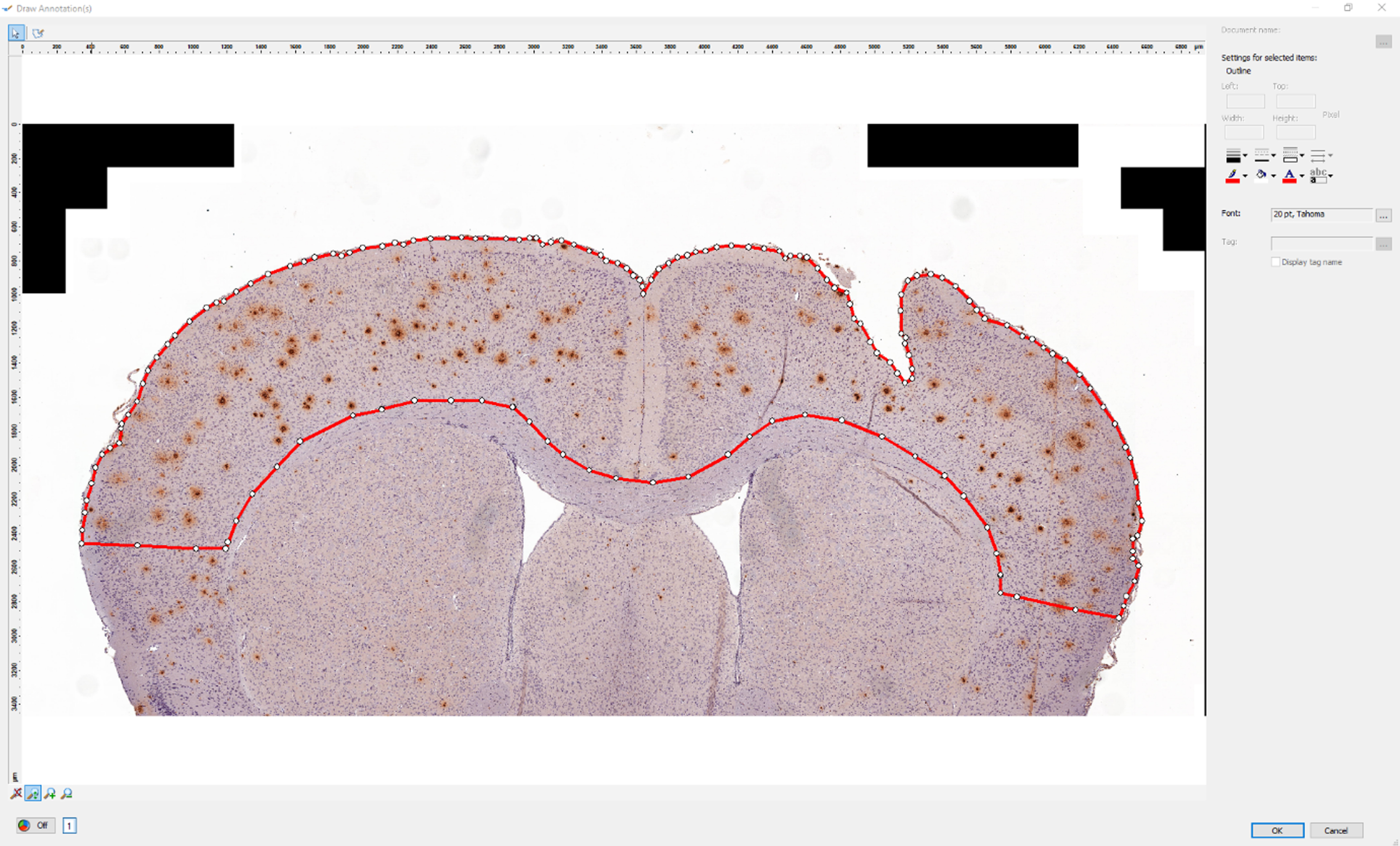
Fig. 2
Defining the hemisphere border. We have marked the upper and lower points where the hemispheres meet (red circles) using the circle tool in our custom script in AxioVision.
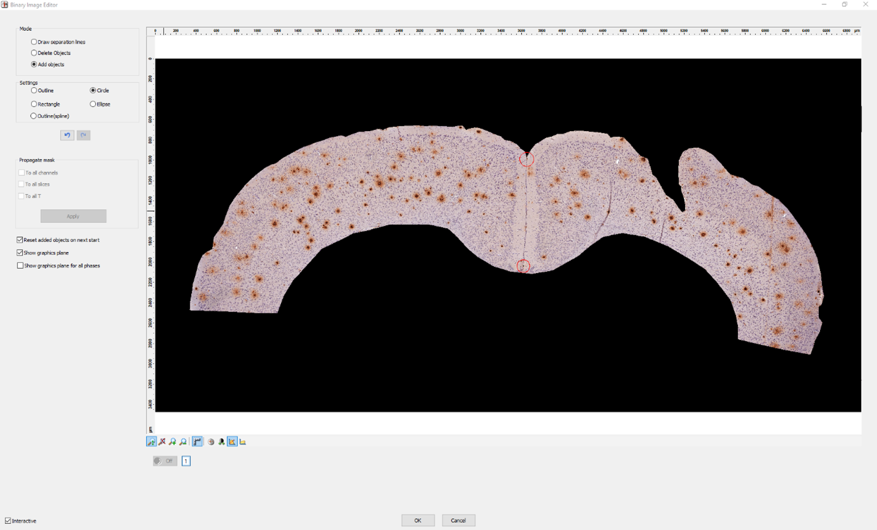
Fig. 3
Defining the injection point. We have defined the injection point and a corresponding point in the contralateral hemisphere (red circles) using our custom script in AxioVision. The previously selected points are displayed in yellow.
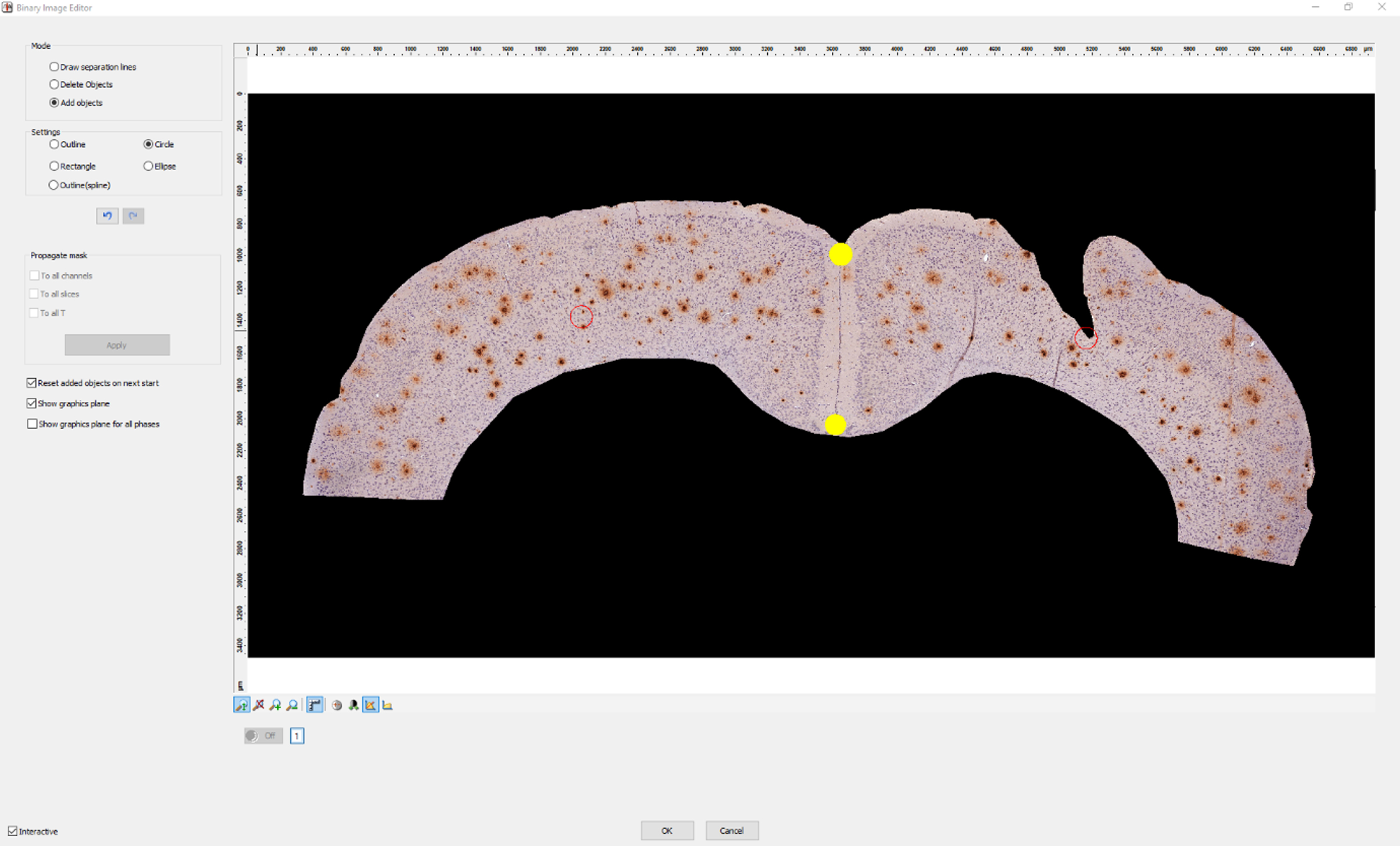
Fig. 4
Separating plaques. How to separate two plaques that have been detected as one object using the line tool in our custom script in AxioVision.
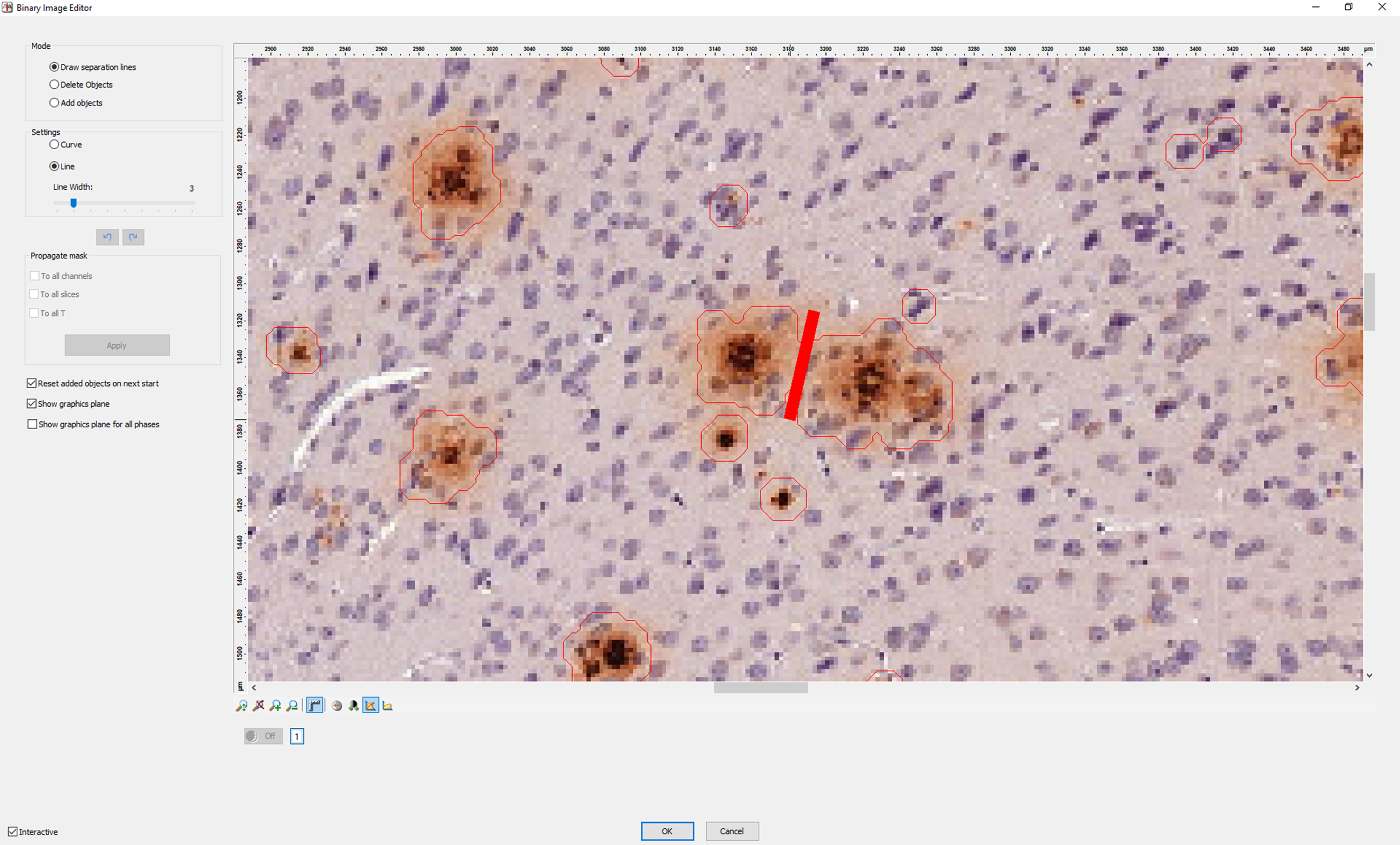
Fig. 5
Removing false positive objects. The outline color of each object indicates whether an object will be included in (green outline) or excluded from (red outline) the subsequent quantification of plaques.

Processing raw data (Excel)
Next, the raw data output from AxioVision is processed and analyzed further using the Excel tool “Pump_Animal-Analysis_Tool_Template.xltm”. In this newly designed tool, we used Power Query data connection technology, and made several folder queries to load the raw data from the exported CSV files. We have included two versions of our tool. First, we provide an empty version that can be used to analyze your own data (Excel macro-enabled template, XLTM, Supplementary Material 3). Second, we provide a version containing sample data for demonstration purposes (Excel macro-enabled workbook, XLSM, Supplementary Material 4).
The following systematic protocol describes in detail how to use the custom Excel tool. It explains how to import and label data. After completing these steps, the user will have prepared the data for analysis and visualization.
Note: The Excel file includes hidden sheets. These hidden sheets are used to filter values needed for the graphs and are not meant to be changed by the general end user.
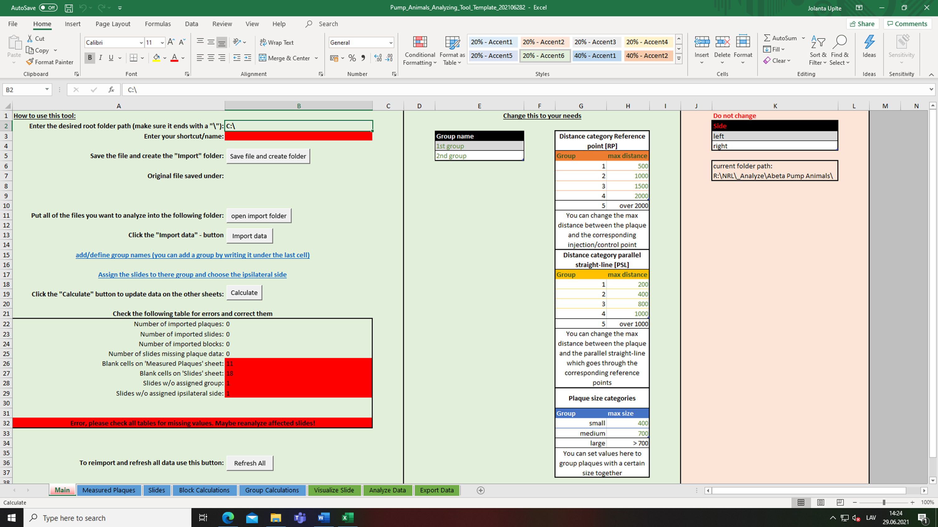
1. Open the Excel tool “Pump_Animals_Analyzing_Tool_Template.xltm” (Supplementary Material 3). When double-clicking onto the file, Excel will open a new instance of the template (Fig. 6).
2. Before you can import your AxioVision raw data, the file needs to be saved. To this end, enter the path where all files should be saved to (“desired root folder” in the worksheet “Main”) and your name/shortcut. Then, click on “Save file and create folder”. This step will create a folder in the selected root folder (“Username_YYYYMMDD”), save the Excel tool as XLSM file (Excel macro-enabled workbook) and create a subfolder “Import”.
3. Next, you have to provide the raw data that you have obtained from AxioVision. Open the import folder and move or copy all CSV files that have been generated during the first part of this protocol (Section 2) into this folder (4 CSV files per slide).
4. You can now start the data import by clicking on the button “Import data”. A macro will extract all data from the files and save them inside the current Excel file.
5. If your data originates from animals in different groups, you can define and label all groups (table “Group name” in the worksheet “Main”). If you have more than two groups, expand the table as needed.
6. Next, provide information about each imported slide. Clicking “Assign the slides to their group and choose the ipsilateral side” brings you to the worksheet “Slides”. Assign each slide to a group (column “Group”) and select the ipsilateral side as noted in section 3 (column “Ipsilateral side”). You can note additional slide-specific comments in the column “info”.
7. Finally, you can customize the distance categories for the following analyses (worksheet “Main”, tables “Distance group reference point [RP]” and “Distance group parallel straight line [PSL]”). We explain the meaning of these categories in Section 5.1. Initially, we recommend keeping the default values.
8. Once you have filled in all required information, start the analysis by pressing the button “Calculate”. You have to repeat this step, if new data is added or any information on the worksheet “Slides” is changed.
9. Note: Should you experience problems or inconsistencies, you can re-calculate everything (worksheet “Main”, button “Refresh all”). During a refresh, all information given in the worksheets “Main” and “Slides” is preserved. Use this script also to add more slides later (after you copied the new CSV files to the “Import” folder).
10. In the worksheet “Main”, you can find basic plausibility checks to verify that all data is imported correctly and has been labelled. If any check fails, the cell will be highlighted in red.
Fig. 6
Starting with our custom Excel tool. Screenshot of the worksheet “Main” with different settings and customizable options. Image shows a new/fresh instance of the template in Microsoft Excel.
Data analysis and data presentation
In the previous sections, we have described how to analyze slides in AxioVision, and how to process and label the obtained raw data in Excel. For the visualization and interpretation of the data, our Excel tool offers different charts and tables (worksheets “Visualize Slide” and “Analyze data”). In the following section, we will provide more details about these worksheets. Moreover, the worksheet “Export Data” provides several pre-defined filters to export specific sets of values for the analysis in third-party software, e.g., statistical analysis in Prism (GraphPad Software, San Diego, CA, USA).
Plaque categorization: “Reference point” and “Parallel straight line”
In this method, we present two different approaches how to characterize plaques based on their distance to a reference point (RP) or to a reference line (parallel straight line, PSL). Both approaches (RP/PSL) categorize plaques in five predetermined distances that can be customized (worksheet “Main”). The detailed mathematical calculations are described in Supplementary Material 1.
Reference point (RP). The RP approach categorizes plaques in a circular manner according to their distance from a reference point (Fig. 7A). On the ipsilateral side, this reference point is the tip of the injected cannula. On the contralateral side, it is the previously selected reference point. The distance categories are defined in the “Main” worksheet. By default, these categories are distances smaller than (1) 500μm, (2) 1000μm, (3) 1500μm, (4) 2000μm, and (5) more than 2000μm.
Fig. 7
Schematic representation of the categorization approaches for amyloid plaques. A) Distance between plaques and the injection point (RP). The RP approach categorizes plaques in a circular manner according to their distance from a reference point. The distance categories are smaller than (1) 500μm, (2) 1000μm, (3) 1500μm, (4) 2000μm, and (5) more than 2000μm. B) The distance between the plaque and the injection channel (PSL). The PSL approach categorizes plaques according to their distance from a reference line. The distance categories are distances smaller than (1) 200μm, (2) 400μm, (3) 800μm, (4) 1000μm, and (5) more than 1000μm. The circles/lines were added manually to visualize the approach and are not used for the actual classification. Representative pictures have been obtained from our custom Excel tool.
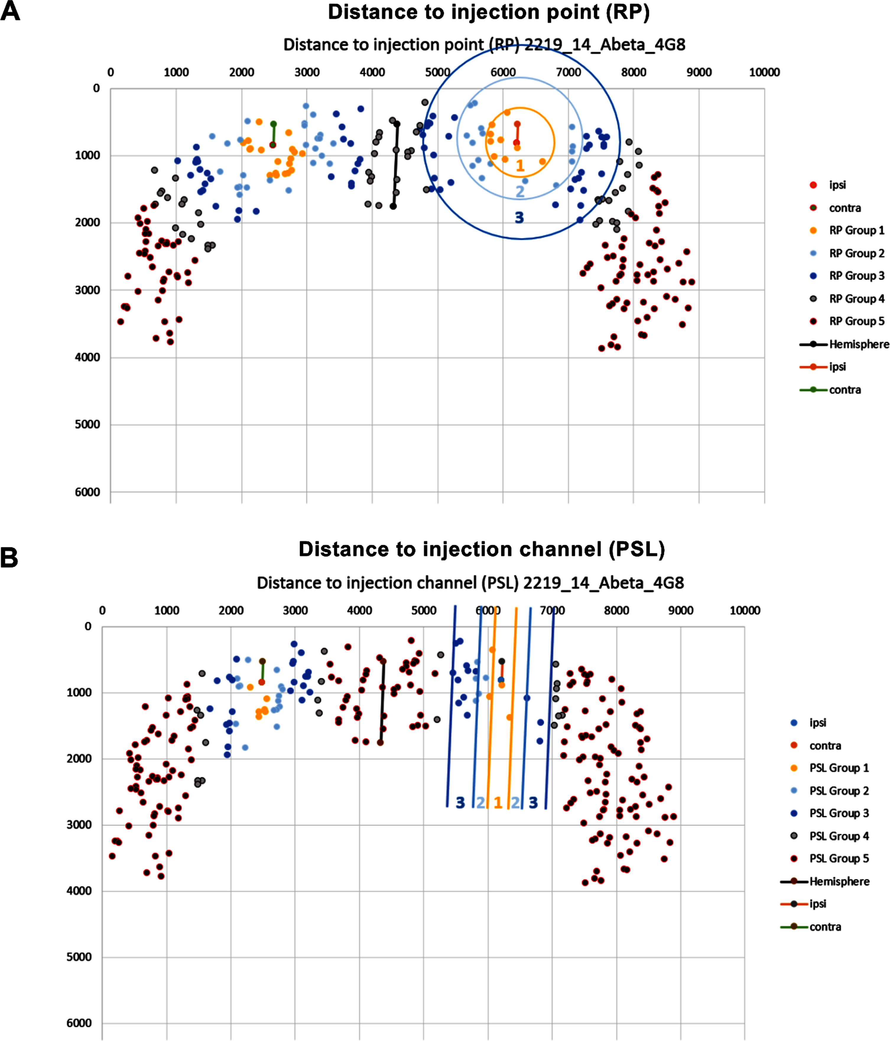
Parallel straight line (PSL). The PSL approach categorizes plaques according to their distance from a reference line. This reference line is calculated as a parallel to the previously defined hemisphere border that goes through the reference point in the respective hemisphere (Fig. 7B). By default, the distance categories are distances smaller than (1) 200μm, (2) 400μm, (3) 800μm, (4) 1000μm, and (5) more than 1000μm.
Visualization of detected plaques
The raw data obtained in AxioVision contains precise two-dimensional coordinates for each plaque, which are used to calculate their distance (RP or PSL). Moreover, we use these coordinates to generate schematic visualizations for one slide at a time (worksheet “Visualize Slide”).
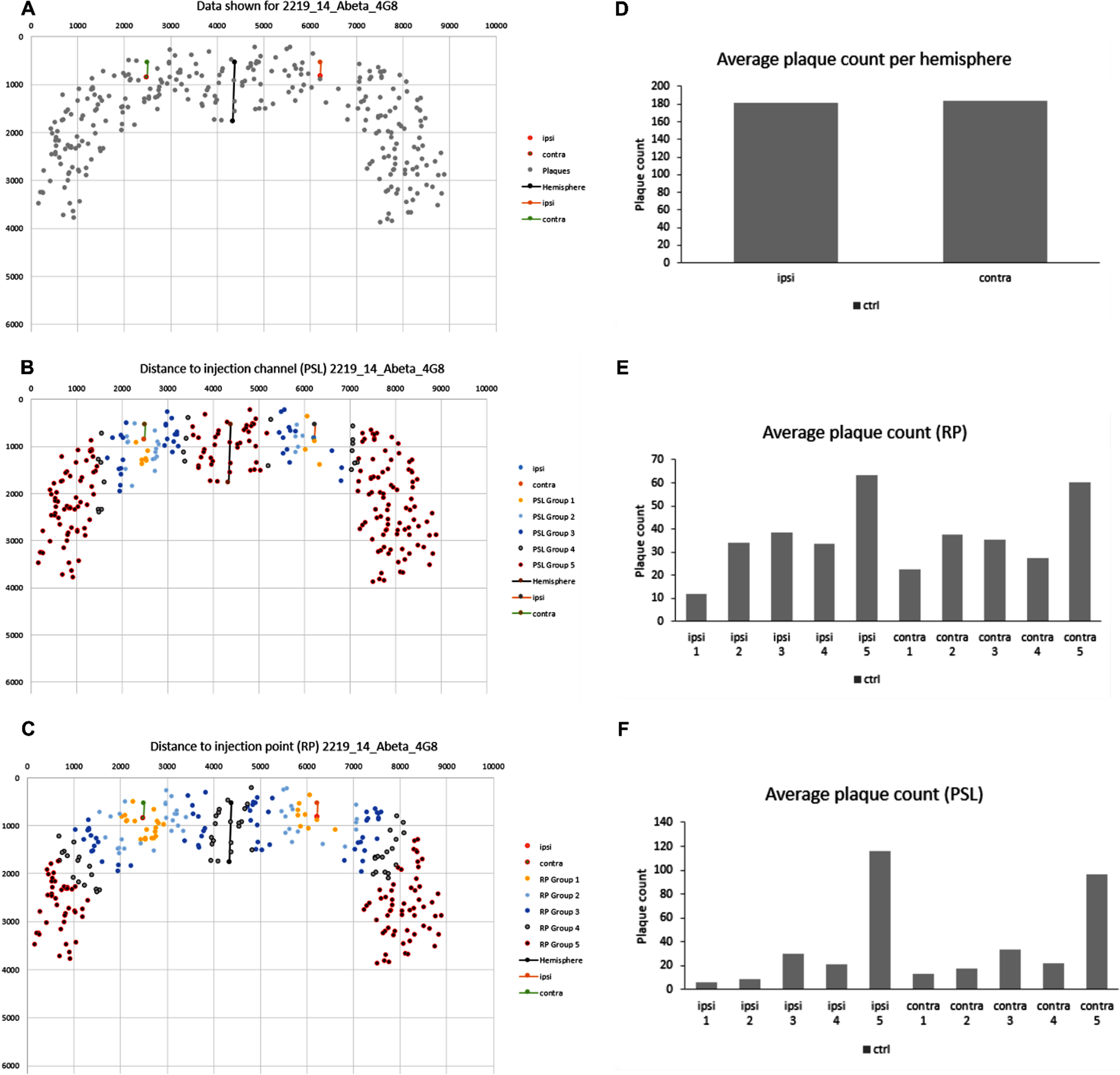
After selecting the slide/animal of interest, the user obtains three different graphs: plaques accumulated across the whole cortex (Fig. 8A), plaques accumulated across the cortex from RP (Fig. 8B) and plaques accumulated across the cortex from PSL (Fig. 8C). Each data point represents one detected plaque, regardless of its size. In Fig. 8A–C, the color of the data points represents their distance to the injection point or channel based on the pre-defined distance groups for RP and PSL.
Fig. 8
Graphical visualization of plaques in the cortex of a mouse in Excel. A) The plaques accumulated across the cortex as detected by AxioVision. B) The plaques accumulated in the cortex categorized by distance group RP. C) The plaques accumulated in the cortex categorized by distance group PSL. D-F) Distance histograms showing the number of plaques. Representative pictures have been obtained from our custom Excel tool.
These graphical representations allow the user to visualize plaque location around the injection point or channel and to detect potential calculation errors, e.g., if quantified plaques do not belong to a particular distance group.
Quantification of detected plaques
Our Excel tool quantifies plaques based on their location alone or in combination of location and size categories (small, medium, large). In the worksheet “Analyze Data”, the user finds several automatically generated charts that display group means of these quantifications. For biological relevance, group means are calculated by first calculating values per slide (worksheet “Slides”), subsequently averaging all slides of one block (i.e., animal, worksheet “Block Calculations”), and finally calculating the mean counts of all animals in the respective group (worksheet “Group calculations”). By default, all groups are selected, but users can deselect groups to display fewer groups in the charts. To exclude individual slides from subsequent calculations, users can remove the group label of the respective slide in the worksheet “Slides”.
Obtained charts include the number of plaques (Fig. 8D), and distance histograms based on the pre-defined distance categories for RP (Fig. 8E) and PSL (Fig. 8F).
Sample data set
To demonstrate the functionality of the Excel tool, we have included a sample data set with this publication. We provide raw data (Supplementary Material 4) and specific graphs (Supplementary Material 5). The sample data was obtained from 16 immunohistochemically stained brain sections from eight animals that received intracerebral injections of PBS using mini-osmotic pumps. The detailed methods are described in Supplementary Material 1 together with an extended description of the results and relevant comparisons. We present the quantitative measures (number of plaques, cortex area covered by plaques and size of plaques) obtained from 1-2 IHC stained brain sections per animal (slides, n = 14; animals, n = 8).
Furthermore, we analyzed the sample data statistically, comparing the ipsi- and contralateral hemispheres (Supplementary Material 5). We present four different quantitative measurements: number of plaques, size of plaques, number of plaques by size groups, and cortex area covered by plaques. The Excel template categorizes plaques according to their size: 1) small, ≤400μm2; 2) medium, 401–700μm2; 3) large, > 700μm2, according to Bolmont et al. [20]. Additionally, the Excel template calculates the number of plaques for each size group in the pre-defined distance groups RP and PSL. The in-depth analysis of plaques according to size and location allows us to detect whether a particular plaque category has decreased around the injection site induced by the administered compound.
DISCUSSION
Since Aβ plays a major role in the initiation and progression of AD, several methods have been developed to perform quantitative analysis of Aβ aggregates and to investigate the therapeutic efficacy of treatment in transgenic mouse models [21]. The delivery of proteins and pharmacological compounds into the brain are important strategies for studying mechanisms underlying brain diseases and evaluating candidate molecules for new treatments. However, drug-delivery to the brain is challenging due to the BBB [22]. It is well recognized that the route of administration is a critical determinant of the final pharmacokinetics, pharmacodynamics as well as toxicity of pharmacological agents. Intravenous, subcutaneous, intraperitoneal, and oral routes are the main paths of drug administration in laboratory animals, each offering advantages and disadvantages depending on specific goals of the preclinical studies [23]. However, for long-term experiments with purified drugs, systemic administration by intraperitoneal injection is not considered the preferred choice for targeting the brain, as it induces stress in rodents and requires high doses of drugs [23, 24]. In this context, mini-osmotic pumps represent an ideal system for studying long-term treatments in the brain, at a fixed known delivery rate that eludes the problem of daily injection stress in animals and overcomes the BBB by direct intracerebroventricular administration [17, 18, 25, 26].
Proper formulation of a drug and appropriate route of administration are crucial for preclinical and clinical success at later stages of drug development. Potential routes of administration are usually addressed after proof-of-concept studies where the goal is to evaluate the effects of target engagement [23]. Intracerebroventricular administration of agents using mini-osmotic pumps (e.g., ALZET) is a well-established method. ALZET pumps have been used in thousands of studies on the effects of controlled delivery of a wide range of experimental agents, including peptides, hormones, growth factors, and antibodies [27–29]. Due to the unique mechanism by which ALZET pumps operate, compounds of any molecular conformation can be delivered predictably at controlled rates, independent of their physical and chemical properties [18]. So far, published studies have selected different neuroanatomical sites of interest that are close to the cannula insertion channel (e.g., various hippocampal regions) as regions of interest (cortex and hippocampus) and they are mainly involved in memory-related processes [30, 31]. Most of the studies applying intracerebral injections focus on assessing the hippocampus or even smaller regions of interest. Considering the limited size of these regions, quantification of Aβ plaques and evaluation of a potential treatment are less complex, especially if the target tissue has not been traumatized [32–35]. Other quantitative methods require homogenized brain tissue, e.g., ELISA or western blot, or the separation of both hemispheres of the brain to perform immunohistochemistry or biochemical studies [36–38]. However, these methods can provide a complete visual comparison of the distribution of plaques between the control and the injected hemisphere, further determining the possible distribution of treatment. There is very limited data available regarding how the quantification of Aβ plaques should be performed in relation to intracerebral injection channels. Therefore, we developed a suitable analytical tool, which performs histopathological quantification, e.g., in the entire cortex area and compares the results of both hemispheres after continuous long-term intracerebral injection using mini-osmotic pumps.
Our tool analyzes and evaluates Aβ plaques in specific brain areas based on their location relative to the point of injection or the injection channel. The analysis tool enables reporting of additional data based on the ROI, number, and sizes of the selected Aβ plaques. We also developed worksheets for quality control and visualization of data obtained in AxioVision. Additionally, using PBS-treated experimental animals as proof of concept, we obtained results about Aβ plaque distribution in our model. It is important to find out whether a potential treatment could reduce the number of a specific plaque size based on the ROI. The core functionality of our tool is the classification of Aβ plaques in pre-defined distance groups by two different approaches (reference point, RP, and parallel straight line, PSL) and different plaque sizes (small, medium, large), that allows us to gain a better understanding of potential treatment effectiveness. Essentially, this functionality could serve as a basis for more specific and accurate determination of the distribution and efficacy of the newly tested substances.
The developed tool serves as an alternative approach to deliver a more accurate technique to analyze histological images and quantify Aβ plaques therein, especially after long-term intracerebral injection by using mini-osmotic pumps. Different other methods exist that have been used to quantify Aβ plaques, but in general, these processing and analyzing tools (e.g., AxioVision, ImageJ) do not provide strategies for specific situations with lost tissue and injection trajectories. The presented toolbox enables the user to share information faster, more accurate and more detailed, especially when tissue has been damaged and the location effect relative to the drug distribution is needed.
The tool presented here can be applied to many types of injections such as stereotactic microinjections, intracortical injections and ventricular injections [17, 18, 25, 26, 39]. While our analysis is focused on plaque analysis, our method can be used to determine various other immunohistochemical markers, e.g., intracellular neurofibrillary tangles composed of highly phosphorylated forms of the protein tau, or markers related to neuroinflammation, including the astrocyte marker glial fibrillary acidic protein (GFAP), and the microglia marker ionized calcium-binding adaptor molecule–1 (IBA1). The tool might also be useful to analyze in vivo approaches with side differences where potentially a part of the tissue is lost. Trauma or stroke models could be tested to be analyzed with the toolbox; after induction of a head injury, the size of the traumatized tissue region is reduced as compared to the non-traumatized brain hemisphere [40, 41].
However, we would also like to point out some limitations of our method. One limitation of the AxioVision tool is the need of user involvement to segregate manually double plaques by drawing a line between the single plaques that have not been separated automatically. In addition, the user needs to carefully check the automatic recognition and deselect/select the affected objects and decide whether the recognized object is a real plaque or not. As both mentioned aspects are involved in the analysis of the Aβ plaques, there is a possibility that the user intervention to identify errors and to separate plaques may lead to additional errors in the results (user error). Automatic image analysis can help to increase objectivity and reduce time, e.g., machine learning-supported analyses (DeePathology™ STUDIO) can reduce the effort needed for analysis showing comparable quantitative results to the traditional approach [42, 47]. Equally important is that although the Excel tool provides a graphical visualization of the Aβ plaques and their categorization into different distance groups, an important addition would be to recognize the plaque sizes (based on size groups small, medium, large) in distance groups [43–46].
From a technical standpoint, our method could be optimized for better comparison between experimental groups by calculating automatically the RP on the contralateral side (mirrored along the hemisphere border). Another improvement would be to make the number of distance categories customizable.
In conclusion, our study has demonstrated that this analytic tool improves performance of evaluation process for potential treatments after continuous long-term intracerebral injection in vivo studies. However, further studies are necessary to generate representative results obtained with our new method that would increase its current usage and potential impact.
ACKNOWLEDGMENTS
This work was supported by the Latvian Council of Science Fund, project (ShortAbeta), project No. lzp-2018/1-0275.
The work of J.P. was also supported by the following grants: Deutsche Forschungsgemeinschaft/ Germany (DFG 263024513); Ministerium für Wirtschaft und Wissenschaft und Digitalisierung Sachsen-Anhalt/ Germany (ZS/2016/05/78617); Nasjonalforeningen (16154), HelseSØ/ Norway (2019054, 2019055); Barnekreftforeningen (19008); EEA grant/Norges grants (TAČR TARIMAD TO100078); Norges forskningsrådet/ Norway (260786 PROP-AD, 295910 NAPI, 327571 PETABC); European Commission (643417).
PROP-AD and PETABC are EU Joint Programme –Neurodegenerative Disease Research (JPND) projects.
PROP-AD is supported through the following funding organizations under the aegis of JPND – http://www.jpnd.eu (AKA #301228 –Finland, BMBF #01ED1605 –Germany, CSO-MOH #30000-12631 –Israel, NFR #260786 –Norway, SRC #2015-06795 –Sweden).
PETABC is supported through the following funding organizations under the aegis of JPND –https://www.jpnd.eu (NFR #327571 –Norway, FFR #882717 –Austria, BMBF #01ED2106 –Germany, MSMT #8F21002–Czech Republic, VIAA #ES RTD/2020/26 –Latvia, ANR #20-JPW2-0002-04 –France, SRC #2020-02905 –Sweden). The projects receive funding from the European Union’s Horizon 2020 research and innovation programme under grant agreement #643417 (JPco-fuND).
Authors’ disclosures available online (https://www.j-alz.com/manuscript-disclosures/21-5180r1).
SUPPLEMENTARY MATERIAL
[1] The supplementary material is available in the electronic version of this article: https://dx.doi.org/10.3233/JAD-215180.
REFERENCES
[1] | Cummings J ((2021) ) New approaches to symptomatic treatments for Alzheimer’s disease. Mol Neurodegener 16: , 2. |
[2] | Scheltens P , De Strooper B , Kivipelto M , Holstege H , Chetelat G , Teunissen CE , Cummings J , van der Flier WM ((2021) ) Alzheimer’s disease. Lancet 397: , 1577–1590. |
[3] | Boese AC , Hamblin MH , Lee JP ((2020) ) Neural stem cell therapy for neurovascular injury in Alzheimer’s disease. Exp Neurol 324: , 113112. |
[4] | Weidling IW , Swerdlow RH ((2020) ) Mitochondria in Alzheimer’s disease and their potential role in Alzheimer’s proteostasis. Exp Neurol 330: , 113321. |
[5] | John A , Reddy PH ((2021) ) Synaptic basis of Alzheimer’s disease: Focus on synaptic amyloid beta, P-tau and mitochondria. Ageing Res Rev 65: , 101208. |
[6] | Cosacak MI , Bhattarai P , Kizil C ((2020) ) Alzheimer’s disease, neural stem cells and neurogenesis: Cellular phase at single-cell level. Neural Regen Res 15: , 824–827. |
[7] | Rao CV , Asch AS , Carr DJJ , Yamada HY ((2020) ) “Amyloid-beta accumulation cycle” as a prevention and/or therapy target for Alzheimer’s disease. Aging Cell 19: , e13109. |
[8] | Harris JR ((2005) ) The contribution of microscopy to the study of Alzheimer’s disease, amyloid plaques and Abeta fibrillogenesis. Subcell Biochem 38: , 1–44. |
[9] | Antzutkin ON ((2004) ) Amyloidosis of Alzheimer’s Abeta peptides: Solid-state nuclear magnetic resonance, electron paramagnetic resonance, transmission electron microscopy, scanning transmission electron microscopy and atomic force microscopy studies. Magn Reson Chem 42: , 231–246. |
[10] | Kreplak L ((2016) ) Introduction to atomic force microscopy (AFM) in biology. Curr Protoc Protein Sci 85: , 17.7.1–17.7.21. |
[11] | Ha C , Park CB ((2006) ) Ex situ atomic force microscopy analysis of beta-amyloid self-assembly and deposition on a synthetic template. Langmuir 22: , 6977–6985. |
[12] | Hung LW , Ciccotosto GD , Giannakis E , Tew DJ , Perez K , Masters CL , Cappai R , Wade JD , Barnham KJ ((2008) ) Amyloid-beta peptide (Abeta) neurotoxicity is modulated by the rate of peptide aggregation: Abeta dimers and trimers correlate with neurotoxicity. J Neurosci 28: , 11950–11958. |
[13] | Bruggink KA , Muller M , Kuiperij HB , Verbeek MM ((2012) ) Methods for analysis of amyloid-beta aggregates. J Alzheimers Dis 28: , 735–758. |
[14] | Laloux C , Gouel F , Lachaud C , Timmerman K , Do Van B , Jonneaux A , Petrault M , Garcon G , Rouaix N , Moreau C , Bordet R , Duce JA , Devedjian JC , Devos D ((2017) ) Continuous cerebroventricular administration of dopamine: A new treatment for severe dyskinesia in Parkinson’s disease? Neurobiol Dis 103: , 24–31. |
[15] | Choi JY , Yeo IJ , Kim KC , Choi WR , Jung JK , Han SB , Hong JT ((2018) ) K284-6111 prevents the amyloid beta-induced neuroinflammation and impairment of recognition memory through inhibition of NF-kappaB-mediated CHI3L1 expression. J Neuroinflammation 15: , 224. |
[16] | Gunther EC , Smith LM , Kostylev MA , Cox TO , Kaufman AC , Lee S , Folta-Stogniew E , Maynard GD , Um JW , Stagi M , Heiss JK , Stoner A , Noble GP , Takahashi H , Haas LT , Schneekloth JS , Merkel J , Teran C , Naderi ZK , Supattapone S , Strittmatter SM ((2019) ) Rescue of transgenic Alzheimer’s pathophysiology by polymeric cellular prion protein antagonists. Cell Rep 26: , 145–158.e8. |
[17] | Dong X ((2018) ) Current strategies for brain drug delivery. Theranostics 8: , 1481–1493. |
[18] | Gullapalli R , Wong A , Brigham E , Kwong G , Wadsworth A , Willits C , Quinn K , Goldbach E , Samant B ((2012) ) Development of ALZET(R) osmotic pump compatible solvent compositions to solubilize poorly soluble compounds for preclinical studies. Drug Deliv 19: , 239–246. |
[19] | Sike A , Wengenroth J , Upite J , Bruning T , Eiriz I , Santha P , Biverstal H , Jansone B , Haugen HJ , Krohn M , Pahnke J ((2017) ) Improved method for cannula fixation for long-term intracerebral brain infusion. J Neurosci Methods 290: , 145–150. |
[20] | Bolmont T , Haiss F , Eicke D , Radde R , Mathis CA , Klunk WE , Kohsaka S , Jucker M , Calhoun ME ((2008) ) Dynamics of the microglial/amyloid interaction indicate a role in plaque maintenance. J Neurosci 28: , 4283–4292. |
[21] | Ayton S , Bush AI ((2021) ) beta-amyloid: The known unknowns. Ageing Res Rev 65: , 101212. |
[22] | Zhou X , Smith QR , Liu X ((2021) ) Brain penetrating peptides and peptide-drug conjugates to overcome the blood-brain barrier and target CNS diseases. Wiley Interdiscip Rev Nanomed Nanobiotechnol 13: , e1695. |
[23] | Al Shoyaib A , Archie SR , Karamyan VT ((2019) ) Intraperitoneal route of drug administration: Should it be used in experimental animal studies? Pharm Res 37: , 12. |
[24] | Matzneller P , Kussmann M , Eberl S , Maier-Salamon A , Jager W , Bauer M , Langer O , Zeitlinger M , Poeppl W ((2018) ) Pharmacokinetics of the P-gp inhibitor tariquidar in rats after intravenous, oral, and intraperitoneal administration. Eur J Drug Metab Pharmacokinet 43: , 599–606. |
[25] | Sanchez-Mendoza EH , Carballo J , Longart M , Hermann DM , Doeppner TR (2016) Implantation of miniosmotic pumps and delivery of tract tracers to study brain reorganization in pathophysiological conditions. J Vis Exp, e52932. |
[26] | Glascock JJ , Osman EY , Coady TH , Rose FF , Shababi M , Lorson CL (2011) Delivery of therapeutic agents through intracerebroventricular (ICV) and intravenous (IV) injection in mice. J Vis Exp, 2968. |
[27] | Zweckberger K , Ahuja CS , Liu Y , Wang J , Fehlings MG ((2016) ) Self-assembling peptides optimize the post-traumatic milieu and synergistically enhance the effects of neural stem cell therapy after cervical spinal cord injury. Acta Biomater 42: , 77–89. |
[28] | Schneider MP , Sartori AM , Ineichen BV , Moors S , Engmann AK , Hofer AS , Weinmann O , Kessler TM , Schwab ME ((2019) ) Anti-Nogo-A antibodies as a potential causal therapy for lower urinary tract dysfunction after spinal cord injury. J Neurosci 39: , 4066–4076. |
[29] | Yan T , Xiong W , Huang F , Zheng F , Ying H , Chen JF , Qu J , Zhou X ((2015) ) Daily injection but not continuous infusion of apomorphine inhibits form-deprivation myopia in mice. Invest Ophthalmol Vis Sci 56: , 2475–2485. |
[30] | Preston AR , Eichenbaum H ((2013) ) Interplay of hippocampus and prefrontal cortex in memory. Curr Biol 23: , R764–773. |
[31] | Chen Y , Guo Z , Mao YF , Zheng T , Zhang B ((2018) ) Intranasal insulin ameliorates cerebral hypometabolism, neuronal loss, and astrogliosis in streptozotocin-induced Alzheimer’s rat model. Neurotox Res 33: , 716–724. |
[32] | Sepulveda MR , Dresselaers T , Vangheluwe P , Everaerts W , Himmelreich U , Mata AM , Wuytack F ((2012) ) Evaluation of manganese uptake and toxicity in mouse brain during continuous MnCl2 administration using osmotic pumps. Contrast Media Mol Imaging 7: , 426–434. |
[33] | Pasetto L , Pozzi S , Castelnovo M , Basso M , Estevez AG , Fumagalli S , De Simoni MG , Castellaneta V , Bigini P , Restelli E , Chiesa R , Trojsi F , Monsurro MR , Callea L , Malesevic M , Fischer G , Freschi M , Tortarolo M , Bendotti C , Bonetto V ((2017) ) Targeting extracellular cyclophilin A reduces neuroinflammation and extends survival in a mouse model of amyotrophic lateral sclerosis. J Neurosci 37: , 1413–1427. |
[34] | Tang C , Guo W ((2021) ) Implantation of a mini-osmotic pump plus stereotactical injection of retrovirus to study newborn neuron development in adult mouse hippocampus. STAR Protoc 2: , 100374. |
[35] | Diaz-Aparicio I , Paris I , Sierra-Torre V , Plaza-Zabala A , Rodriguez-Iglesias N , Marquez-Ropero M , Beccari S , Huguet P , Abiega O , Alberdi E , Matute C , Bernales I , Schulz A , Otrokocsi L , Sperlagh B , Happonen KE , Lemke G , Maletic-Savatic M , Valero J , Sierra A ((2020) ) Microglia actively remodel adult hippocampal neurogenesis through the phagocytosis secretome. J Neurosci 40: , 1453–1482. |
[36] | Wen TC , Lall S , Pagnotta C , Markward J , Gupta D , Ratnadurai-Giridharan S , Bucci J , Greenwald L , Klugman M , Hill NJ , Carmel JB ((2018) ) Plasticity in one hemisphere, control from two: Adaptation in descending motor pathways after unilateral corticospinal injury in neonatal rats. Front Neural Circuits 12: , 28. |
[37] | Zhou L , Li Q (2019) Isolation of region-specific microglia from one adult mouse brain hemisphere for deep single-cell RNA sequencing. J Vis Exp, doi: 10.3791/60347. |
[38] | Krohn M , Bracke A , Avchalumov Y , Schumacher T , Hofrichter J , Paarmann K , Frohlich C , Lange C , Bruning T , von Bohlen Und Halbach O , Pahnke J ((2015) ) Accumulation of murine amyloid-beta mimics early Alzheimer’s disease. Brain 138: , 2370–2382. |
[39] | McSweeney C , Mao Y ((2015) ) Applying stereotactic injection technique to study genetic effects on animal behaviors. J Vis Exp e52653. |
[40] | Xie BS , Wang YQ , Lin Y , Mao Q , Feng JF , Gao GY , Jiang JY ((2019) ) Inhibition of ferroptosis attenuates tissue damage and improves long-term outcomes after traumatic brain injury in mice. CNS Neurosci Ther 25: , 465–475. |
[41] | Willis EF , MacDonald KPA , Nguyen QH , Garrido AL , Gillespie ER , Harley SBR , Bartlett PF , Schroder WA , Yates AG , Anthony DC , Rose-John S , Ruitenberg MJ , Vukovic J ((2020) ) Repopulating microglia promote brain repair in an IL-6-dependent manner. Cell 180: , 833–846.e816. |
[42] | Bascunana P , Brackhan M , Pahnke J ((2021) ) Machine learning-supported analyses improve quantitative histological assessments of amyloid-beta deposits and activated microglia. J Alzheimers Dis 79: , 597–605. |
[43] | Kepe V , Huang SC , Small GW , Satyamurthy N , Barrio JR ((2006) ) Visualizing pathology deposits in the living brain of patients with Alzheimer’s disease. Methods Enzymol 412: , 144–160. |
[44] | Barrio JR , Kepe V , Satyamurthy N , Huang SC , Small G ((2008) ) Amyloid and tau imaging, neuronal losses and function in mild cognitive impairment. J Nutr Health Aging 12: , 61S–65S. |
[45] | Stolte C , Sabir KS , Heinrich J , Hammang CJ , Schafferhans A , O’Donoghue SI ((2015) ) Integrated visual analysis of protein structures, sequences, and feature data. BMC Bioinformatics 16 Suppl 11: , S7. |
[46] | Lee SP , Falangola MF , Nixon RA , Duff K , Helpern JA ((2004) ) Visualization of beta-amyloid plaques in a transgenic mouse model of Alzheimer’s disease using MR microscopy without contrast reagents. Magn Reson Med 52: , 538–544. |
[47] | MöhleL , BascuñanaP, BrackhanM, PahnkeJ ((2021) ) Development of deep learning models for microglia analyses in brain tissue using DeePathology™ STUDIO. J Neurosci Methods. Dec 1;364: :109371. doi: 10.1016/j.jneumeth.2021.109371. PMID: 34592173 |


