
Near-Infrared Optical Spectroscopy In Vivo Distinguishes Subjects with Alzheimer’s Disease from Age-Matched Controls
Abstract
Background:
Medical imaging methods such as PET and MRI aid clinical assessment of Alzheimer’s disease (AD). Less expensive, less technically demanding, and more widely deployable technologies are needed to expand objective screening for diagnosis, treatment, and research. We previously reported brain tissue near-infrared optical spectroscopy (NIR) in vitro indicating the potential to meet this need.
Objective:
To determine whether completely non-invasive, clinical, NIR in vivo can distinguish AD patients from age-matched controls and to show the potential of NIR as a clinical screen and monitor of therapeutic efficacy.
Methods:
NIR spectra were acquired in vivo. Three groups were studied: autopsy-confirmed AD, control and mild cognitive impairment (MCI). A feature selection approach using the first derivative of the intensity normalized spectra was used to discover spectral regions that best distinguished “AD-alone” (i.e., without other significant neuropathology) from controls. The approach was then applied to other autopsy-confirmed AD cases and to clinically diagnosed MCI cases.
Results:
Two regions about 860 and 895 nm completely separate AD patients from controls and differentiate MCI subjects according to the degree of impairment. The 895 nm feature is more important in separating MCI subjects from controls (ratio-of-weights: 1.3); the 860 nm feature is more important for distinguishing MCI from AD (ratio-of-weights: 8.2).
Conclusion:
These results form a proof of the concept that near-infrared spectroscopy can detect and classify diseased and normal human brain in vivo. A clinical trial is needed to determine whether the two features can track disease progression and monitor potential therapeutic interventions.
INTRODUCTION
Although research has increased our understanding of the cellular pathology of Alzheimer’s disease (AD), little progress has been made towards therapy [1] because the insidious onset of symptoms masks the ongoing, irreversible damage until a diagnosis can be established. Clinical assessment of dementia relies upon neurological, neuropsychological, and imaging data for diagnoses of probable AD or senile dementia of the Alzheimer type. Such cases can be provided with a definitive diagnosis of AD only by postmortem neuropathological examination of brain tissue. Positron emission tomography (PET) and magnetic resonance imaging (MRI) have significantly advanced AD research and medical diagnosis [2]. Contrast provided by exogenous radionuclide markers (PET) or the hydrogen atoms of endogenous water molecules (MRI) enable high resolution images to be constructed, which accurately represent neuropathological features of AD: neurofibrillary tangles and amyloid plaques in the case of PET, or cortical atrophy characteristic of the progressive neurodegeneration of AD in the case of MRI. Dynamic processes altered in AD such as glucose utilization and regional hemoglobin oxygenation may be monitored by FDG-PET and BOLD-MRI, respectively [2].
The inherent physical and chemical properties of AD pathology also alter the optical spectroscopic features of the tissue in diseased brain compared to non-diseased brain. For example, consider a figurative comparison between the hallmark histopathological features of AD, plaques and tangles in the neuropil, and water droplets in the atmosphere. These dense protein aggregates of tau (tangles) and amyloid-β (plaques) are uncharacteristic of the surrounding neuropil with respect to both size and relative refractive index. Similarly, water droplets in the atmosphere, when compared to the surrounding air, are also large dense aggregates with a different refractive index. In both cases, light scattering and refraction contribute to a wavelength dependent angular redistribution of the light, i.e., a spectrum. The observed spectrum is dependent on whether the water droplets are present—for example a rainbow—or not, and likewise on whether AD is present or not—for example the diffuse scattering spectra we report here. To be clear, this is not a claim that we are reporting detection of plaques and tangles but rather an illustration of how diffuse scattering of near-infrared light by brain tissue may be altered in AD. Of particular note is that since this effect is due to inherent physical chemical properties, exogenous markers are not required.
A non-invasive method that screens for changes in the structure and composition of brain tissue might allow for early detection and also assess the effects of early interventions, which could greatly accelerate the development of treatments and prevention. Optical spectroscopy can capture chemical and structural information non-invasively and near-infrared spectroscopy in particular can usefully probe deeper layers of tissue. Near-infrared light propagates several centimeters in tissue to reach the brain from the surface of the scalp, because these wavelengths are only weakly absorbed and largely forward scattered [3]. Although most applications of near-infrared spectroscopy to the head involve oximetry [4–7] or blood flow [8–10], more recent advances have included imaging [11–14] and co-registration studies [15–17]; hemoglobin spectroscopy is central to most of these techniques. In contrast, our laboratory has been studying spectroscopy as a method to detect the chemical and structural changes of AD [18, 19], with an eye toward classification or taxonomy. In short, for the purposes of the familiar near-infrared methods listed above, hemoglobin’s spectral characteristics are signal; for our taxonomic purposes, they are noise [20, 21]. Supplementary Table 1 lists known scatters and absorbers of brain tissue.
In collaboration with Boston University’s Alzheimer’s Disease Center, we first demonstrated that near-infrared diffuse reflectance spectroscopy distinguishes autopsy samples of brains with AD from those without [20]. We extended this approach to living subjects by utilizing the relative transparency of biological tissue to light in the 650–1050 nm range[22, 23], a region known as the near-infrared window. A brief overview of how this was done will facilitate the presentation of issues that affected the experimental design. For the acquisition of data, two fiber optic probes are positioned at the same temple, one delivering light from the source and one collecting diffusely reflected light and delivering it to the detector. With a separation of 25 mm between the delivering and collecting probes, the light signal that is detected and analyzed has interrogated a portion of the temporal lobe as well as overlying tissues [3, 24, 25]. We acquired spectra from dementia subjects while they were alive and used only those for whom postmortem examination confirmed the diagnosis of AD. Control and MCI subjects had volunteered for the Boston University Alzheimer’s Disease Center’s HOPE [26] protocol, which evaluates the cognitive function of its subjects annually. Although acquiring the spectra is straightforward, analyzing them encounters two major difficulties: the similarity of the spectra from different groups and the presence of multiple neuropathological co-morbidities in individual subjects.
To appreciate the first issue requires understanding a general principle [27], often left unstated, that motivates applications of optical spectroscopy to medical diagnosis: if the same light source illuminates two distinct materials, the resultant spectra are a priori distinct.
Therefore, it is expected that the spectra from AD and normal brains will differ. In practice, however, the scattering of light from biological tissues often renders it extremely difficult to discover those spectral features that mark the difference [5, 27–29]. To mitigate this first problem, we eventually adopted algorithms from the field of feature selection (also called pattern recognition) [30–32] to search for those regions of the spectra that best distinguished two groups, that is, those regions of taxonomic signal.
The second issue of multiple neuropathological co-morbidities in the brains of the elderly [33] was confirmed by the autopsy reports. To mitigate this problem, we identified subjects who had AD (NIA-Reagan [34]: high likelihood; Braak neurofibrillary stage [35]: VI) but no other significant pathology, the closest to “pure AD” in practice, whose spectra became our standard. We shall refer to these as “AD-alone,” that is, AD without significant additional neuropathology. Feature selection on spectra of AD-alone versus control subjects suggested two features that were adequate for classification of all participants, even those with additional pathology such as infarcts and Lewy bodies. Therefore, the results reported here constitute a proof of the concept that NIR spectroscopy can usefully classify AD in vivo. The utility of this concept in practice must be determined by a clinical trial that monitors subjects longitudinally.
METHODS
Spectroscopy
Diffuse scattering spectra from 650–1050 nm were acquired using the clinical spectrometer system we are developing. Two fiber optic probes designed in-house and using optical fiber elements and manufacturing from both Fiberguide Industries, Caldwell, ID, USA (AFS200/220T) and PolyMicro Technologies, Phoenix, AZ, USA (FBP200220240, FBP600660710) are positioned at the subject’s temple area, using a spacing template constructed for that purpose and held in place by an elastic headband. The source probe (single fiber, low-OH, 600μm core, NA = 0.22) delivers near-infrared light from a continuous-wave tungsten halogen source (HL2000, 20W, Ocean Optics, Dunedin, FL, USA), and the detector probe (multiple fibers, low-OH, 200μm cores, NA = 0.22) collects the diffusely scattered light at various source-detector separations (10–30 mm in 5 mm increments) and conducts it to an imaging spectrograph (HS-F/1.8-NIR, Kaiser Optical Systems, Ann Arbor, MI, USA) coupled to a CCD detector cooled to –50°C (DU-420-OE, Andor Technologies, South Windsor, CT, USA). In this paper we will focus on spectra acquired with the 25 mm source-detector separation because they contain the most taxonomic signal.
For comparison, analysis of data from the 30 mm measurements is presented in the Supplementary Material.
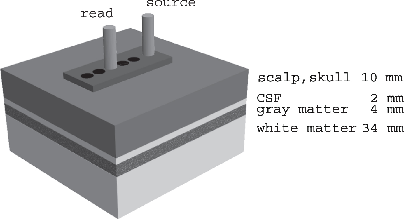
The clinical spectra reported here were acquired in two sessions, with approximately two years between them. A different detector probe was used in each session. Spectra were acquired in the patient’s room or a nearby clinical area, darkened to minimize ambient light interference. Spectra were acquired at each source-detector separation on each temple (Fig. 1). The temple is chosen for two reasons: 1) the greatest loss of neurons in AD occurs in the frontal and temporal lobes [36]; and 2) the temporal bone is thin. Each spectrum was corrected for background and acquisition time; correction for lamp output and detector response was achieved by a reference spectrum obtained by reflection from barium sulphate (first session) or from a Spectralon (SRT-02-050, Labsphere, North Sutton, NH) low reflectance standard (second session). A detailed description of the treatment of raw data is given in the Supplementary Material, Section 2.
Fig. 1
Schematic diagram of method for acquiring spectra. At each temple, spectra are obtained at a range of source-detector separations determined by the plastic template (10–30 mm). The 20 mm source-detector configuration is illustrated; the 25 mm spectra are analyzed in this report. The greater the source-detector separation the greater the depth of the mean photon path. The tissues probed and their nominal thicknesses are labelled. For the 25 mm source-detector separation, the mean photon path includes a portion of the gray matter, in this case part of the temporal lobe.
Participants
Subjects were recruited as part of an ongoing project to monitor the progression of neurodegenerative diseases, especially AD. All subjects were recruited through a process approved by the Institutional Review Boards; informed consent was obtained in all cases. Subjects clinically diagnosed with senile dementia of the Alzheimer’s type were recruited from the inpatient dementia unit of the VA Bedford Healthcare System. All autopsies were performed by one of us (A.C.M.). Routine methods for pathologic processing of tissue and neuropathologic evaluation have been described elsewhere[37]. Briefly, the following stains were used: Luxol fast blue, hematoxylin and eosin, and Bielschowsky’s silver stain.
Immunohistochemical methods for hyperphosphorylated tau (p-tau) (AT8), alpha synuclein, amyloid-β (Aβ), and phosphorylated TDP-43 were performed using previously published methods [38–40]. NIA-Reagan criteria [34] and Braak neurofibrillary staging [35] were tabulated. The average delay between spectroscopy measurement and autopsy was 11 months.
Control subjects and those with mild cognitive impairment had volunteered for the Health Outreach Program for the Elderly (HOPE) of the Boston University Alzheimer’s Disease Center. Participants in the HOPE protocol are to undergo cognitive assessment yearly; the results are reviewed and an expert panel assigns a consensus diagnosis. The control subjects were younger (mean age 76.4 years) than the AD subjects (mean age 82.3 years) but we do not believe this to be clinically significant for these data and therefore view them as age-matched groups.
MCI subjects (mean age 80.6 years) were subclassified into more and less severe. Those with consensus ratings of “probable MCI” or “possible MCI” with a Clinical Dementia Rating = 0.5 were grouped as less severe. Those with a consensus rating of possible AD were grouped as more severe. Of the 12 MCI participants, 7 were less severe and 5 were more severe.
Exclusion criteria
Twenty-five dementia subjects came to autopsy. Five were excluded from analysis here. Two had Lewy bodies present in the temporal isocortex, which is included in the light field interrogated by our method. This adds a confounding factor to the optical signal with too few subjects to assess it. All subjects with Lewy bodies outside the temporal isocortex were included. Three excluded subjects had frontotemporal lobar degeneration with different degrees of AD pathology and highly varied additional pathology. These were excluded because each had unique features that prevented ready grouping with others for feature selection.
Therefore, 20 subjects with autopsy-confirmed AD were studied: AD-alone, (7 subjects); AD with infarcts (6 subjects), AD with Lewy bodies (7 subjects). There were 13 control and 12 MCI subjects, none of whom was excluded.
Feature selection
In general, feature selection consists of four stages: 1) the data set is randomly divided into two subsets: one for exploratory analysis, the other for testing hypotheses generated by the exploration; 2) when successful, exploratory analysis suggests features that may be useful; 3) the candidate features are usually optimized in the first subset by constructing weighted combinations of them to achieve the desired outcome; 4) this optimized model is then applied to the second subset and tested. In commonly used terminology, the exploratory and weighting stages are combined, and the first subset is called the “training set.” Feature selection by fraction product (below) applied to distinguish AD-alone and control subjects results in discriminants that do not need any weighting. The commonly used terminology will lead to confusion because there is no “training” to optimize the features found by exploratory analysis. Therefore, we will refer to the first subset as the “discovery set.” The common term used for the second subset, “test set,” remains appropriate and will be used here.
Fraction-product approach
For exploratory analysis, the general principle for classification is to select those features that maximally separate the groups of interest, but there is no uniform method for achieving this [30]. A common approach is to maximize the Mahalanobis distance among the groups [32], and for the univariate case with two groups this reduces to the t-statistic calculated on the two means and variances [41]. However, because of the small numbers of subjects in each group, many high t-values were due to outliers and the associated feature was not useful in separating the two groups. To solve this problem, we devised a median-based approach in which the two group medians were determined and an estimated cut-off calculated by their average. The fraction of each group correctly classified was determined and their product taken as the measure of separation, leading to the name “fraction-product” for this statistic. This approach gave the same results as the t-statistics but with much more efficiency because outliers had less effect. We have recently learned of a paper by Mucciardi and Gose [31] in which they use a median-based method called the “probability of error”, which is similar to our algorithm. A detailed description of the methods of feature selection is given in the Supplementary Material, Section 3.
Feature selection was performed on the first derivative of the area-normalized intensity spectrum; the value of the first derivative at each wavelength will be referred to as the slope variate. The use of the first derivative helps to bring out small changes in a spectrum against a broad background [42, 43], as is the case with tissue spectra. To calculate the first derivative, the spectrum was smoothed by boxcar averaging and the slope computed as a least-squares fit of a straight line through a region of 11 pixels; the slope variate thus calculated was assigned to the center pixel of the 11 pixel region. This method is the Savitzky–Golay algorithm [44] with a first-order polynomial. The slope variates calculated for the spectra of both temples were averaged pointwise (i.e., pixel by pixel). Eleven subjects were measured in both sessions and the values from each session were averaged pointwise before analysis. Because optical phenomena have linewidth, we also required that features show significant efficacy over several contiguous pixels. This additional criterion is unique to optical data and is not a general technique of feature selection.
The following steps comprised the protocol for feature selection. The group of 7 AD-alone subjects was divided into a discovery set (5 subjects) and a test set (2 subjects). Similarly, the 13 controls were divided into discovery (5 subjects) and test (8 subjects) sets. The measure of separation (mean-based or median-based) was determined at each pixel (wavelength) for the two discovery sets. Features of interest were those in which a large t-statistic or fraction-product occurred over at least three contiguous pixels. Further details concerning feature selection are given in the Supplementary Material, Section 4.
Statistical analysis
All statistical calculations used R [45] statistical software. Programs in the “MASS” library were used for linear discriminant analysis (lda) and principle component analysis (prcomp with scale = T). Linear discriminant analysis was not used to calculate scores but only to determine the relative weight of each variate in distinguishing the two groups. The “Hotelling” package was used for the Hotelling T2 test. Welch’s t-test was performed through the R built-in function t.test.
RESULTS
NIR diffuse reflectance spectra
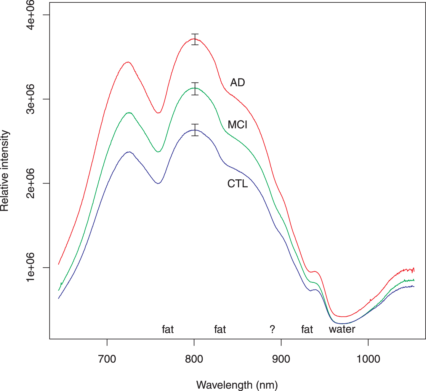
Because first derivative spectra are not familiar to many scientists, the usual intensity spectra (corrected for background, integration time and lamp spectrum) are shown in Fig. 2 as a group average spectrum for each group: autopsy-confirmed AD, MCI, and control. Common spectral features attributed to absorption by fat and water are marked. There is a feature at 895 nm that we have been unable to associate with any biochemical substance. Though the average intensities differ for the three groups, intensities of the individual spectra, which comprise the averages, were found to be less useful for classifying subjects. It is for this reason that we pursued feature selection on the first derivative spectra.
Fig. 2
Average of intensity spectra for all subjects in each group. These intensity spectra have been corrected for background, lamp spectrum, and integration time. The AD spectra include all participants who had autopsy-confirmed AD. The MCI spectra similarly include all subjects regardless of severity. Several features of the spectra may be attributed to well-known absorption by fat or water as marked. There is a shoulder around 895 nm (marked by ?); we have not been able to associate this feature with any biochemical substance. The features used elsewhere in this report come from normalizing the individual spectra to unit area and taking the first derivative. Although the relative intensity of a spectrum could be incorporated as a feature to classify subjects, it is not as efficient as the slope variates. The error bars represent standard error of the mean.
Analysis of selected slope variate features: autopsy-confirmed AD and control
To find the best spectral features for classification, we applied two feature selection algorithms—one using the mean, the other the median—to the AD-alone and control discovery sets, and both gave similar results. Two candidate regions emerged: one centered around 895 nm (spanning 3 pixels), the other around 860 nm (spanning 4 pixels). Linear discriminant analysis [46] determined that the slope variates at 895.68 and 860.64 nm contributed the most to distinguishing AD-alone from control. An unweighted scatter plot of these two variates is shown in Fig. 3. The two features are uncorrelated (Pearson’s product-moment correlation: 0.13 AD-alone; –0.15 controls). For both the discovery and test sets, the AD-alone and control points fall within two well-separated regions of the diagram, which confirms the utility of the chosen slope variates for classification.
Fig. 3
Scatter plot of selected AD and control subjects. To minimize confounding factors, we performed feature selection to distinguish subjects with AD-alone from controls. Following the usual approach of feature selection, the subjects were divided into two sets: one used to identify the classifiers (here called discovery) and the other to confirm (test). Both discovery and test sets behave similarly and will not be distinguished in subsequent figures. Parenthetical number is the number of subjects in that group.
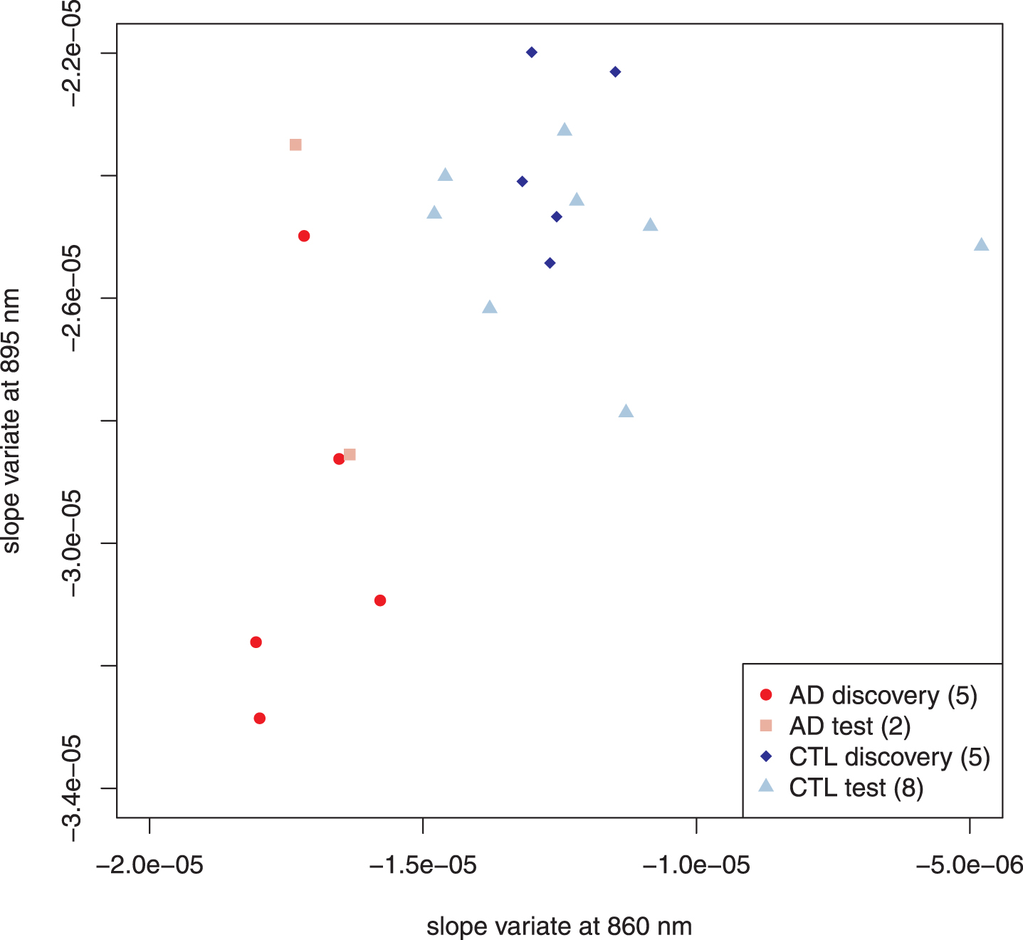
Figure 4 illustrates the addition of autopsy confirmed subjects that had a high likelihood of AD by the NIA-Reagan criteria but also had significant other pathology: infarcts (6 subjects) or Lewy bodies (7 subjects). Dispersion of the data points increases, as expected, but they remain within the same two regions of the plot that distinguished AD-alone from controls. Comparison of all cases that had no role in feature selection showed statistically significant separation between AD and control (15 autopsy confirmed AD cases; 8 control cases; p < 0.0003, Hotelling’s T2-test; see Table 1 for all compared sets).
Fig. 4
Scatter plot adding AD subjects with additional pathology. The addition of the subjects with other pathology increases the dispersion in the AD group but the points remain within the same regions as the previous diagram. Points distinguished as “test” in Fig. 3 have been combined with the discovery set. Parenthetical number is the number of subjects in that group.
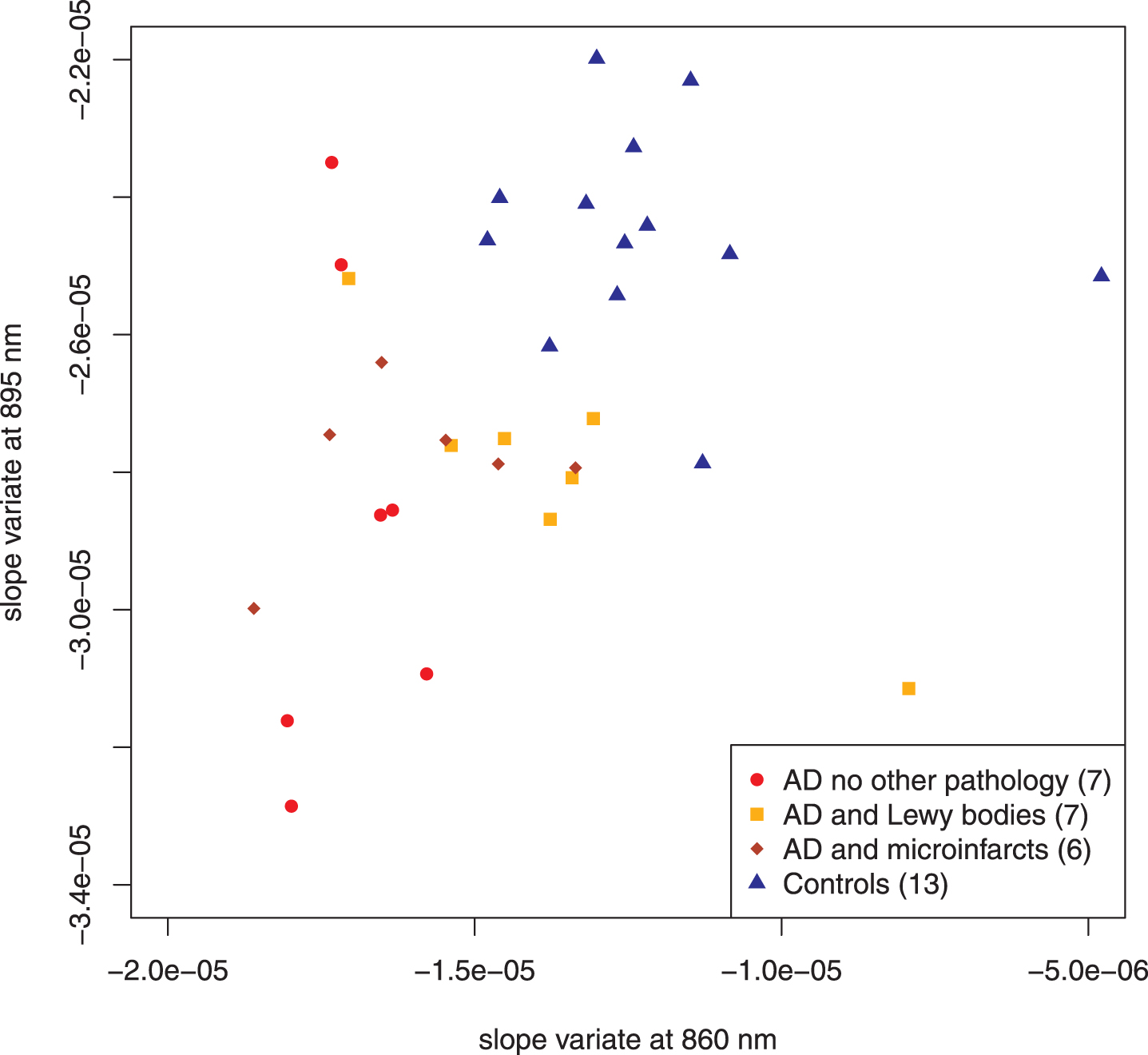
Table 1
Number of Subjects in Discovery Sets and Test Sets together with Statistical Comparison
| Discovery Sets | Test Sets | |||||
| Control | AD alone | Control | AD alone | AD + infarcts | AD + LBs | |
| 5 | 5 | 8 | 2 | 6 | 7 | |
| Control | All Test AD | p-value | ||||
| Hotelling T2 test | 8 | 15 | <0.0003 | |||
AD, Alzheimer’s disease; LBs, Lewy bodies.
Analysis of selected slope variate features: MCI subjects
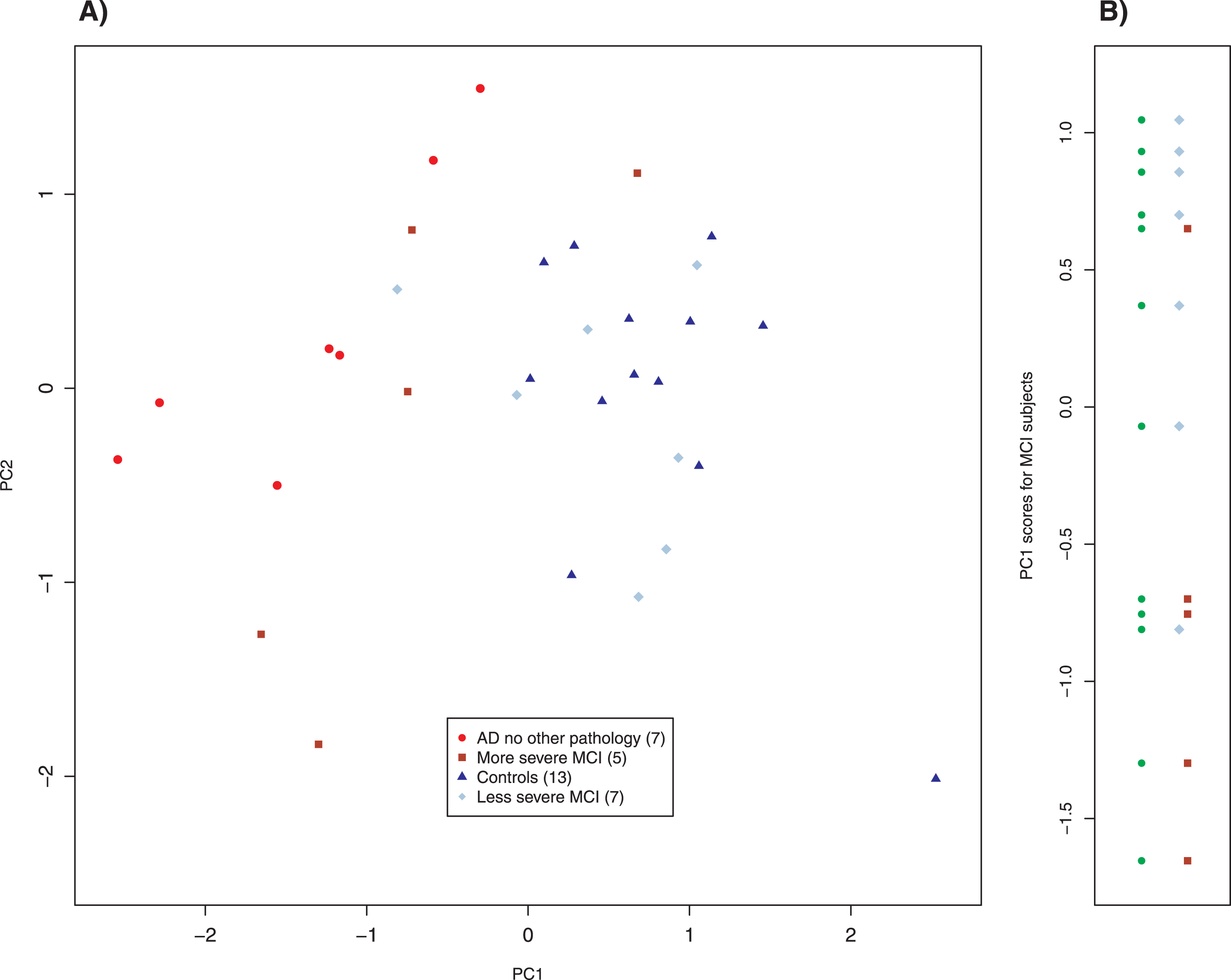
We also studied 12 subjects with mild cognitive impairment (MCI) whom we clinically subclassified as more severe (5 subjects) and less severe (7 subjects). Their results are plotted in Fig. 5. The more and less severe MCI subjects appear to cluster similarly to the AD and control scatter plots but were shifted slightly down and to the left; note that the axes in Figs. 3–5 are identical. Application of linear discriminant analysis to MCI and control groups suggested that 895 nm was the better discriminant (ratio of weights: 1.3), whereas MCI and AD-alone returned 860 nm as the better discriminant (ratio of weights: 8.2). To determine whether proper weighting of the two slope variates might clarify the relationship among MCI, control and AD-alone, we performed principal component analysis (PCA) on those three groups. PCA is a standard method of data analysis that in this setting may be viewed as fitting a straight line to the data by the method of least squares [47]. This line and that normal to it become a new set of axes for displaying the data (Fig. 6A). The new axes are called the first and second principal components (PC1 and PC2), and the new co-ordinates of the points are often called “scores.” The new axes are mean-centered (the mean being for all three groups) and are a linear combination of the previous axes, that is, two differently weighted combinations of the two slope variates (Fig. 6A). For our data, what is most important is that the classification of a point (AD, MCI, control) plays absolutely no role in determining either the principal components or the scores. Although the new variates are weighted combinations of the old, the weights are not selected to optimize a particular outcome; therefore, this is not training. Examining the MCI scores displayed in Panel B of Fig. 6 simply as points (filled circles) leads to the conclusion that they tend to cluster into two groups; by contrary hypotheses, they would have clustered about their mean value in the new coordinates or have been uniformly distributed along the axis. When our clinical assessments are factored in, it is clear that the clusters correspond to those that are more and less impaired, with two exceptional points (Fig. 6B). When the PC1 scores are used to characterize the MCI subjects that we have clinically subclassified, the separation of the more and the less impaired is statistically significant (Welch’s t-test, p < 0.041), even though two subjects are misclassified.
Fig. 5
Scatter plot of MCI subjects. The regional clustering is similar to that of AD and control but is shifted slightly. The axes of Figs. 3, 4, and 5 are identical. Parenthetical number is the number of subjects in that group.
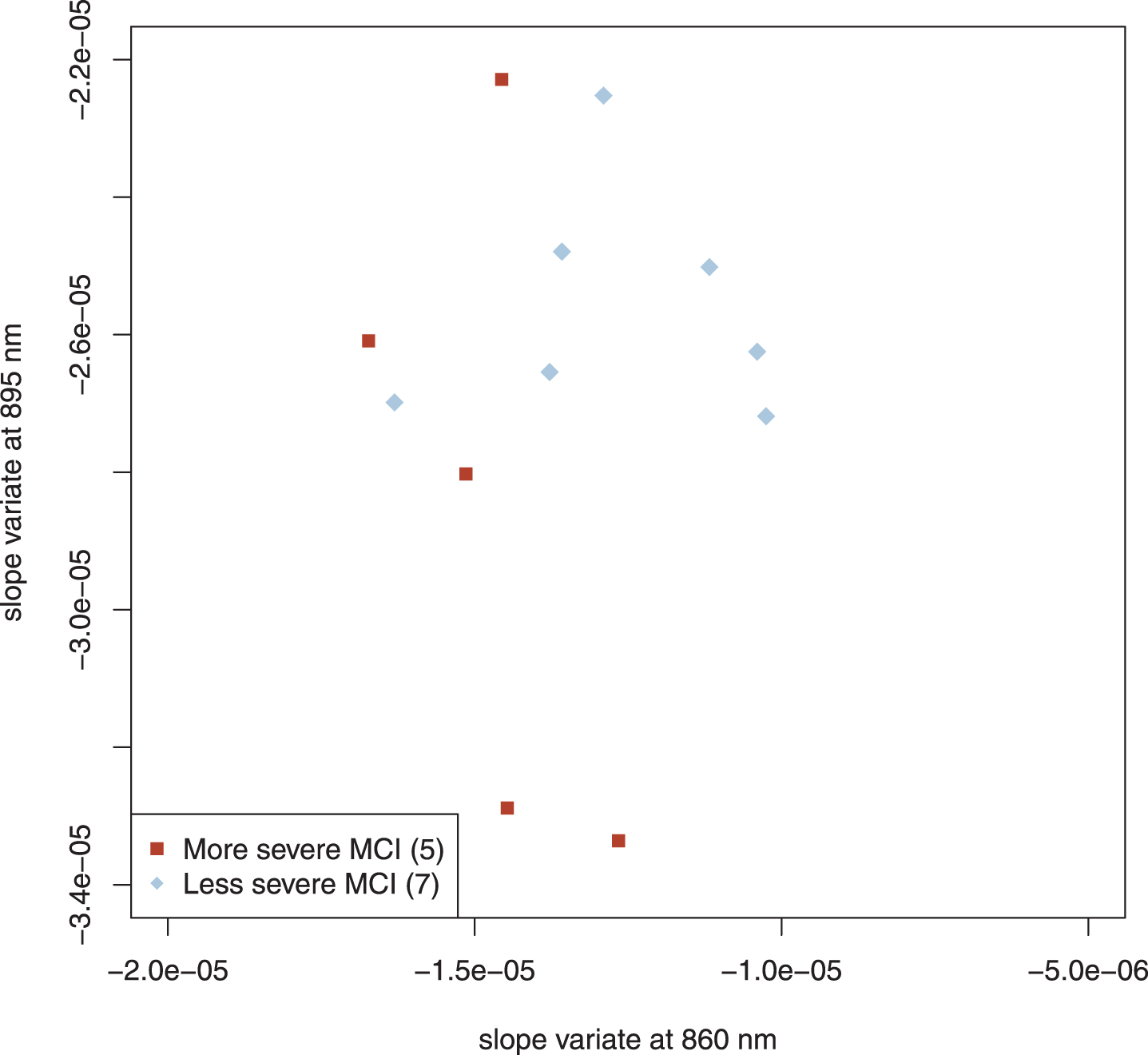
Fig. 6
Principal component analysis of MCI, control, and AD without other pathology subjects. The left panel is a biplot of the principal component analysis. The right panel shows the distribution of MCI subjects using the scores of PC1 as a parameter. The left column of points (filled circles) shows that there is a tendency for the MCI subjects to separate into two groups, which correspond to the clinical classification of severity (right column). Two pairs of overlapping points have been slightly displaced for clarity. Parenthetical number is the number of subjects in that group.
Analysis of excluded subjects
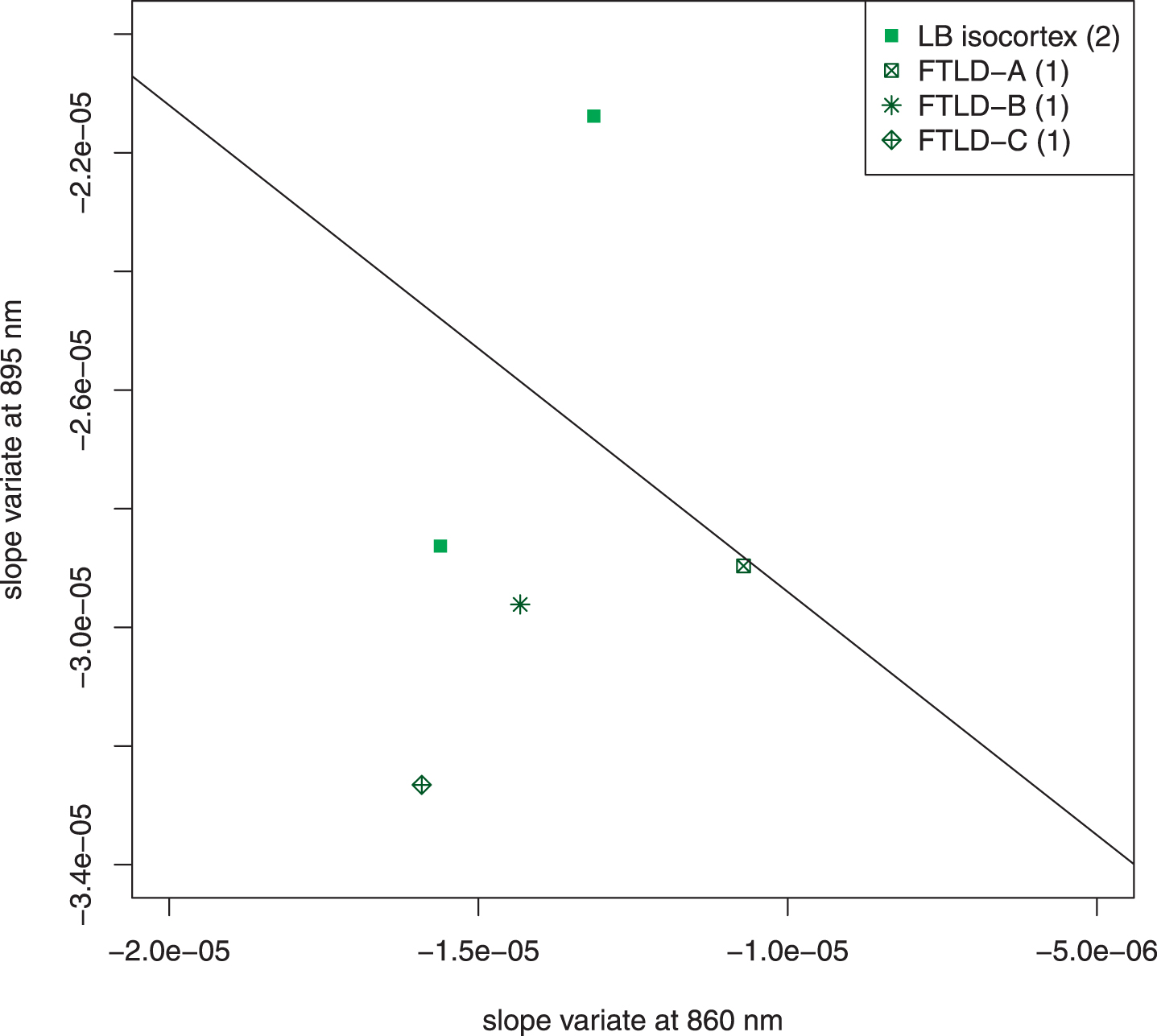
Figure 7 is an unweighted scatter plot of the subjects that were excluded because of confounding structures in the light field (Lewy bodies in the temporal isocortex) or highly heterogenous pathology with frontotemporal lobar degeneration. The scatter plot shows that the overall conclusions of the previous analysis are not affected but that the presence of Lewy bodies in the temporal isocortex can contribute to the misclassification of a subject with autopsy-confirmed AD.
Fig. 7
Scatter plot of excluded subjects. Five subjects who came to autopsy were excluded because of unique features of their pathology. Two had Lewy bodies in the temporal isocortex; both of these were NIA-Reagan high likelihood, Braak VI. Three had frontotemporal lobar degeneration (FTLD) with other pathology. FTLD-A, NIA-Reagan intermediate likelihood, Braak IV; FTLD-B, tau-type, NIA Reagan high likelihood, Braak stage VI, Lewy bodies; FTLD-C, TDP 43 positive inclusions (including temporal cortex), Lewy bodies, 1 + neuritic plaques. The line drawn separates the AD subjects from the control subjects in Fig. 4. The exclusion of these subjects did not affect the overall interpretation of the data. It is noteworthy that the two most extreme cases (LB isocortex on control side of line and FTLD-C) both had pathologic structures in temporal cortex, which adds a confounding factor to the optical signal.
Similarity of results from 30 mm source-detector spectra
The primary purpose of this paper is to present the 25 mm spectra as a proof of concept. However, the light detected at the 30 mm source-detector separation also probes a portion of the temporal lobe. To illustrate the variation with source-detector separation, we applied the analysis used on the 25 mm data (same discovery set, test set, excluded subjects) to the 30 mm spectra. The data are given in the Supplementary Material; only the significant results are presented here.
Feature selection using AD-alone and control groups led to the selection of the same two slope variates at 895.68 and 860.64 nm; the scatter plot of the unweighted variates also completely separated the two groups (Supplementary Figure 1). Addition of AD subjects with additional pathology increases the dispersion, and in contrast to the 25 mm plot, there is now some overlap between control and AD subjects (Supplementary Figure 2).
Nonetheless, the separation of the test groups of AD and control remains statistically significant (p < 0.003; Hotelling T2 test). PCA of AD-alone, control and MCI subjects leads to scores that usefully classify MCI subjects (Supplementary Figure 3B). Again, there are two subjects misclassified, but the separation between the two groups is statistically significant (p < 0.03; Welch t-test). LDA again demonstrates that signal at 895 nm plays a more important role in distinguishing MCI from control subjects (ratio of weights 2.5) whereas the slope variate at 860 better separates MCI from pure AD (ratio of weights 1.5).
DISCUSSION
Starting with 5 AD-alone subjects and 5 controls, we discovered two spectral features that distinguish AD from control. The 10 test set subjects (2 AD-alone; 8 control) plotted in Fig. 3 and the 13 dementia subjects subsequently plotted in Fig. 4 played no role in the determination of the features. Nonetheless, these 23 subjects followed the same regional clustering as the 10 members of the discovery set. This marks the first successful classification of a neurodegenerative condition in vivo by near-infrared optical spectroscopy. In a strict sense, the 10 subjects in the discovery set whose spectra were examined by feature selection generated the empirical hypothesis that slope variates at 895.68 and 860.64 nm could usefully separate AD from control; the subsequent analysis of 23 subjects that played no role in feature selection confirms this hypothesis. We prefer the term “discovery set” to the more commonly used “training set” because typically candidate features must be weighted to optimally classify the individuals; the process of determining those optimal weights is a large portion of “training.” For these data, no weighting was required to classify the subjects –no training per se; there was only discovery of features. Moreover, we imposed the additional requirement that the feature be effective over several contiguous pixels in order to increase the likelihood that it would correspond to a true spectroscopic feature with linewidth. Our results are consistent with the discovery of two spectral features that are traceable to chemical and structural differences between the brains of those with AD and controls. Of course, in a clinical sense, it was clear who did and who did not suffer from dementia without the spectroscopic information. However, Fig. 4 does demonstrate that, when viewed from the proper mathematical perspective, you can “see” AD pathology through the near-infrared window.
Excluding AD subjects with additional pathology from the search for useful features was essential because the additional pathology led to confounding spectral features that may also distinguish the dementia subject from controls but that obscured those features that are more specific for AD. Figure 7 shows that those subjects completely excluded from this analysis would not have altered the overall conclusions. The ultimate solution of confounding signals is to obtain enough autopsy results so that most subjects may be classified by NIR spectroscopy; for example, features will be found to determine whether there are abnormal structures in the temporal isocortex and to account for them.
Figure 2 shows at a glance that the three groups (AD, MCI, CTL) are differentiated by the average intensity of diffusely reflected light. This is to be expected because the transparent layer of cerebrospinal fluid (Fig. 1) acts as a light pipe [25, 48, 49] and should increase in thickness as cortical atrophy progresses. The larger the light pipe, the greater the intensity of light at remote distances from the source. However, the intensities of the individual spectra were not useful for classifying cases. Furthermore, the shapes of the three spectra in Fig. 2 appear to be so similar as to be indistinguishable. In order to search for features that are as instrument-independent as possible, we chose the first derivative of the area-normalized intensity spectra, which we refer to as the slope variate. The use of the slope variate strips away as much of the intensity information as possible, leaving what is mathematically close to “pure shape” and hopefully instrument independent. The achievement of instrument- independence is supported by the fact that these measurements were made in two sessions with slightly different experimental conditions: different reference materials for lamp correction and different detector fibers. Of course, the intensity information can be added back if need be, but the success of the slope variates is adequate for classification of these data.
Several facts lead to optimism that these findings may extend to a larger population. First, the significance of the Hotelling T2 test performed on the test subjects (p < 0.0003) factors in the small number of subjects. Second, the MCI participants are also test subjects, and their separation by PCA supports the hypothesis that the selected features correspond to tissue structure and chemistry. Finally, the selection of the same two features in the analysis of the 30 mm data with results consistent with those obtained at 25 mm further strengthens the arguments that the slope variates at 860 and 895 nm answer to biochemical entities; in particular, the Hotelling T2 test performed on the 30 mm test subjects is also statistically significant (p < 0.003).
The fact that PCA shows two clusters of the MCI values that correspond to AD and control groups is important in potential applications. In a physical sense, it means that some MCI patients have brains that are similar to AD brains whereas others have brains similar to controls. These mathematical results are independent of, but consistent with, our clinical assessments. Although Fig. 5 gives a hint of this finding, PCA makes it quantitative. It is most intriguing that the slope variate at 895 nm plays a more important role in distinguishing MCI from control subjects, whereas the slope variate at 860 nm better separates MCI from those with AD. Together with the fact that the two slope variates are uncorrelated, this behavior suggests that the method probes two distinct processes with that at 895 nm being more significant earlier and that at 860 nm playing a more important role later in the progression of AD. We have not been able to identify the tissue structures or biochemistry that underlie the signals at 895 and 860 nm and we decline to speculate. Although this is frustrating, it also opens the possibility of discovering a new factor in the pathophysiology of AD. One way to search would be to enlarge the range of detected wavelengths to include the mid-infrared, where protein structural features may appear. There is a discernible feature in the spectra shown in Fig. 2 that answers to the slope variate at 895 nm and this fact will facilitate identification of the underlying physical origin of that feature. Finally, the fact that the MCI subjects also played no role in feature selection further strengthens the inference that the features correspond to biochemical entities that play an important role in AD.
The data presented here contain no temporal information. Therefore, larger clinical studies on MCI patients are needed to determine whether the spectral changes track progression of the disease in a useful manner. If so, this approach could become a safe, non-invasive method for assessing response to treatments in real time.
The best-case scenario would be if the signal at 895 nm responds to an intervention that prevents the progression of the 860 nm signal. In this best-case scenario, treatments to prevent AD might be developed and their effects documented before the onset of symptoms and before those symptoms become irreversible.
ACKNOWLEDGMENTS
This work was supported by Merit Review Award I01 CX000827 from the U.S. Department of Veterans Affairs, Clinical Sciences Research and Development Service; by Center Core Grant P30 AG013846 from the U.S. Department of Health and Human Services, National Institutes of Health, National Institute on Aging; and by an unrestricted grant from Headwall Photonics, Inc.
The authors thank Jan-Christian Hütter, of the Broad Institute, for critical discussions on feature selection, and the Boston University Alzheimer’s Disease Center for assistance with patient data management and patient recruitment.
Opinions, interpretations, conclusions, and recommendations are those of the authors and are not necessarily endorsed by the Department of Veterans Affairs.
Authors’ disclosures available online (https://www.j-alz.com/manuscript-disclosures/20-1021r3).
SUPPLEMENTARY MATERIAL
[1] The supplementary material is available in the electronic version of this article: https://dx.doi.org/10.3233/JAD-201021.
REFERENCES
[1] | Huang LK , Chao SP , Hu CJ ((2020) ) Clinical trials of new drugs for Alzheimer disease. J Biomed Sci 27: , 18. |
[2] | Young PNE , Estarellas M , Coomans E , Srikrishna M , Beaumont H , Maass A , Venkataraman AV , Lissaman R , Jiménez D , Betts MJ , McGlinchey E , Berron D , O’Connor A , Fox NC , Pereira JB , Jagust W , Carter SF , Paterson RW , Schöll M ((2020) ) Imaging biomarkers in neurodegeneration: Current and future practices. Alzheimers Res Ther 12: , 49. |
[3] | Pifferi A , Contini D , Mora AD , Farina A , Spinelli L , Torricelli A ((2016) ) New frontiers in time- domain diffuse optics, a review. J Biomed Opt 21: , 091310. |
[4] | Jobsis FF ((1977) ) Noninvasive, infrared monitoring of cerebral and myocardial oxygen sufficiency and circulatory parameters. Science 198: , 1264–1267. |
[5] | Young AE , Germon TJ , Barnett NJ , Manara AR , Nelson RJ ((2000) ) Behaviour of near-infrared light in the adult human head: Implications for clinical near-infrared spectroscopy. Br J Anaesth 84: , 38–42. |
[6] | Strangman G , Franceschini MA , Boas DA ((2003) ) Factors affecting the accuracy of near-infrared spectroscopy concentration calculations for focal changes in oxygenation parameters. Neuroimage 18: , 865–879. |
[7] | Firbank M , Elwell CE , Cooper CE , Delpy DT ((1998) ) Experimental and theoretical comparison of NIR spectroscopy measurements of cerebral hemoglobin changes. J Appl Physiol (1985) 85: , 1915–1921. |
[8] | Owen-Reece H , Smith M , Elwell CE , Goldstone JC , Delpy DT ((1996) ) Near-infrared spectroscopy and cerebral hemodynamics.1424; author reply. Crit Care Med 24: , 1424–1425. |
[9] | Selb J , Boas DA , Chan ST , Evans KC , Buckley EM , Carp SA ((2014) ) Sensitivity of near-infrared spectroscopy and diffuse correlation spectroscopy to brain hemodynamics: Simulations and experimental findings during hypercapnia. Neurophotonics 1: , 015005. |
[10] | Shang Y , Li T , Yu G ((2017) ) Clinical applications of near-infrared diffuse correlation spectroscopy and tomography for tissue blood flow monitoring and imaging.. Physiol Meas 38: , R1–R26. |
[11] | Franceschini MA , Joseph DK , Huppert TJ , Diamond SG , Boas DA ((2006) ) Diffuse optical imaging of the whole head. J Biomed Opt 11: , 054007. |
[12] | Arridge SR ((2011) ) Methods in diffuse optical imaging. Philos Trans A Math Phys Eng Sci 369: , 4558–4576. |
[13] | Ancora D , Qiu L , Zacharakis G , Spinelli L , Torricelli A , Pifferi A ((2018) ) Noninvasive optical estimation of CSF thickness for brain-atrophy monitoring. Biomed Opt Express 9: , 4094–4112. |
[14] | Wilson RH , Nadeau KP , Jaworski FB , Tromberg BJ , Durkin AJ ((2015) ) Review of short-wave infrared spectroscopy and imaging methods for biological tissue characterization. J Biomed Opt 20: , 030901. |
[15] | Fazli S , Mehnert J , Steinbrink J , Curio G , Villringer A , Müller KR , Blankertz B ((2012) ) Enhanced performance by a hybrid NIRS-EEG brain computer interface. Neuroimage 59: , 519–529. |
[16] | Huppert TJ , Allen MS , Diamond SG , Boas DA ((2009) ) Estimating cerebral oxygen metabolism from fMRI with a dynamic multicompartment Windkessel model. Hum Brain Mapp 30: , 1548–1567. |
[17] | Huppert TJ , Hoge RD , Diamond SG , Franceschini MA , Boas DA ((2006) ) A temporal comparison of BOLD, ASL, and NIRS hemodynamic responses to motor stimuli in adult humans. Neuroimage 29: , 368–382. |
[18] | Hanlon EB , Itzkan I , Dasari RR , Feld MS , Ferrante RJ , McKee AC , Lathi D , Kowall NW ((1999) ) Near- infrared fluorescence spectroscopy detects Alzheimer’s disease in vitro. Photochem Photobiol 70: , 236–242. |
[19] | Hanlon EB , Manoharan R , Koo TW , Shafer KE , Motz JT , Fitzmaurice M , Kramer JR , Itzkan I , Dasari RR , Feld MS ((2000) ) Prospects for in vivo Raman spectroscopy. Phys Med Biol 45: , R1–59. |
[20] | Hanlon EB , Perelman LT , Vitkin EI , Greco FA , McKee AC , Kowall NW ((2008) ) Scattering differentiates Alzheimer disease in vitro. Opt Lett 33: , 624–626. |
[21] | Hock C , Villringer K , Müller-Spahn F , Wenzel R , Heekeren H , Schuh-Hofer S , Hofmann M , Minoshima S , Schwaiger M , Dirnagl U , Villringer A ((1997) ) Decrease in parietal cerebral hemoglobin oxygenation during performance of a verbal fluency task in patients with Alzheimer’s disease monitored by means of near-infrared spectroscopy (NIRS)–correlation with simultaneous rCBF-PET measurements. Brain Res 755: , 293–303. |
[22] | Rolfe P ((2000) ) In vivo near-infrared spectroscopy. Annu Rev Biomed Eng 2: , 715–754. |
[23] | Delpy DT , Cope M ((1997) ) Quantification in tissue near–infrared spectroscopy. Phil Trans R Soc Lond B 352: , 649–659. |
[24] | Farrell TJ , Patterson MS , Wilson B ((1992) ) A diffusion theory model of spatially resolved, steady- state diffuse reflectance for the noninvasive determination of tissue optical properties In vivo. Med Phys 19: , 879–888. |
[25] | Okada E , Firbank M , Schweiger M , Arridge SR , Cope M , Delpy DT ((1997) ) Theoretical and experimental investigation of near-infrared light propagation in a model of the adult head. Appl Opt 36: , 21–31. |
[26] | Siwek D ((1999) ) The Health Outreach Program for the Elderly (HOPE) database. Alzheimer Dis Assoc Disord 13: (Suppl 1), S101–105. |
[27] | Richards-Kortum R , Sevick-Muraca E ((1996) ) Quantitative optical spectroscopy for tissue diagnosis. Annu Rev Phys Chem 47: , 555–606. |
[28] | Tuchin VV ((2016) ) Polarized light interaction with tissues. J Biomed Opt 21: , 71114. |
[29] | Pifferi A , Torricelli A , Bassi A , Taroni P , Cubeddu R , Wabnitz H , Grosenick D , Moller M , Macdonald R , Swartling J , Svensson T , Andersson-Engels S , van Veen RL , Sterenborg HJ , Tualle JM , Nghiem HL , Avrillier S , Whelan M , Stamm H ((2005) ) Performance assessment of photon migration instruments: The MEDPHOT protocol. Appl Opt 44: , 2104–2114. |
[30] | Fu KS ((1968) ) Sequential Methods in Pattern Recognition and Machine Learning, Academic Press, Inc, New York. |
[31] | Mucciardi AN , Gose EE ((1971) ) A comparison of seven techniques for choosing subsets of pattern recognition properties. IEEE Trans Comp 20: , 1023–1031. |
[32] | Inza I , Larrañaga P , Saeys Y ((2007) ) A review of feature selection techniques in bioinformatics. Bioinformatics 23: , 2507–2517. |
[33] | Attems J , Jellinger K ((2013) ) Neuropathological correlates of cerebral multimorbidity. Curr Alzheimer Res 10: , 569–577. |
[34] | Hyman BT , Phelps CH , Beach TG , Bigio EH , Cairns NJ , Carrillo MC , Dickson DW , Duyckaerts C , Frosch MP , Masliah E , Mirra SS , Nelson PT , Schneider JA , Thal DR , Thies B , Trojanowski JQ , Vinters HV , Montine TJ ((2012) ) National Institute on Aging-Alzheimer’s Association guidelines for the neuropathologic assessment of Alzheimer’s disease. Alzheimers Dement 8: , 1–13. |
[35] | Braak H , Braak E ((1997) ) Diagnostic criteria for neuropathologic assessment of Alzheimer’s disease. Neurobiol Aging 18: , S85–88. |
[36] | Tomlinson BE ((1992) ) Ageing and the dementias. In Green-field’s Neuropathology, Adams JH, Duchen LW, ed. Oxford University Press, New York, pp. 1284–1410. |
[37] | Vonsattel JP , Aizawa H , Ge P , DiFiglia M , McKee AC , MacDonald M , Gusella JF , Landwehrmeyer GB , Bird ED , Richardson EP Jr. , et al. ((1995) ) An improved approach to prepare human brains for research. J Neuropathol Exp Neurol 54: , 42–56. |
[38] | McKee AC , Cairns NJ , Dickson DW , Folkerth RD , Dirk Keene C , Litvan I , Perl DP , Stein TD , Vonsattel J-P , Stewart W , Tripodis Y , Crary JF , Bieniek KF , Dams-O’Connor K , Alvarez VE , Gordon WA , TBI/CTE group ((2016) ) The first NINDS/NIBIB consensus meeting to define neuropathological criteria for the diagnosis of chronic traumatic encephalopathy. Acta Neuropathol 131: , 75–86. |
[39] | McKee AC , Cantu RC , Nowinski CJ , Hedley-Whyte ET , Gavett BE , Budson AE , Santini VE , Lee H-S , Kubilus CA , Stern RA ((2009) ) Chronic traumatic encephalopathy in athletes: Progressive tauopathy after repetitive head injury. J Neuropathol Exp Neurol 68: , 709–735. |
[40] | McKee AC , Stein TD , Nowinski CJ , Stern RA , Daneshvar DH , Alvarez VE , Lee H-S , Hall G , Wojtowicz SM , Baugh CM , Riley DO , Kubilus CA , Cormier KA , Jacobs MA , Martin BR , Abraham CR , Ikezu T , Reichard RR , Wolozin BL , Budson AE , Goldstein LE , Kowall NW , Cantu RC ((2012) ) The spectrum of disease in chronic traumatic encephalopathy. Brain 136: , 43–64. |
[41] | Das P , Roychowdhury A , Das S , Roychoudhury S , Tripathy S ((2020) ) sigFeature: Novel significant feature selection method for classification of gene expression data using support vector machine and t statistic. Front Genet 11: , 247. |
[42] | Rojas FS , Ojeda CB , Pavon JMC ((1988) ) Derivative ultraviolet—visible region absorption spectrophotometry and its analytical applications. Talanta 35: , 753–761. |
[43] | Bosch Ojeda C , Sanchez Rojas F ((2013) ) Recent applications in derivative ultraviolet/visible absorption spectrophotometry: 2009–2011: A review. Microchem J 106: , 1–16. |
[44] | Savitzky A , Golay MJE ((1964) ) Smoothing and differentiation of data by simplified least squares procedures. Anal Chem 36: , 1627–1639. |
[45] | R Development Core Team (2019) R foundation for Statistical Computing, Vienna, Austria. |
[46] | Fisher RA ((1936) ) The use of multiple measurements in taxonomic problems. Ann Eugen 7: , 179–188. |
[47] | Pearson K ((1901) ) On lines and planes of closest fit to systems of points in space. Philos Mag 2: , 559–572. |
[48] | Okada E , Delpy DT ((2003) ) Near-infrared light propagation in an adult head model. I. Modeling of low-level scattering in the cerebrospinal fluid layer. Appl Opt 42: , 2906–2914. |
[49] | Okada E , Delpy DT ((2003) ) Near-infrared light propagation in an adult head model. II. Effect of superficial tissue thickness on the sensitivity of the near-infrared spectroscopy signal. Appl Opt 42: , 2915–2922. |

