
Detection and Prediction of Mild Cognitive Impairment in Alzheimer’s Disease Mice
Abstract
Background:
The recent failure of clinical trials to treat Alzheimer’s disease (AD) indicates that the current approach of modifying disease is either wrong or is too late to be efficient. Mild cognitive impairment (MCI) denotes the phase between the preclinical phase and clinical overt dementia. AD mouse models that overexpress human amyloid-β (Aβ) are used to study disease pathogenesis and to conduct drug development/testing. However, there is no direct correlation between the Aβ deposition, the age of onset, and the severity of cognitive dysfunction.
Objective:
To detect and predict MCI when Aβ plaques start to appear in the hippocampus of an AD mouse.
Methods:
We trained wild-type and AD mice in a Morris water maze (WM) task with different inter-trial intervals (ITI) at 3 months of age and assessed their WM performance. Additionally, we used a classification algorithm to predict the genotype (APPtg versus wild-type) of an individual mouse from their respective WM data.
Results:
MCI can be empirically detected using a short-ITI protocol. We show that the ITI modulates the spatial learning of AD mice without affecting the formation of spatial memory. Finally, a simple classification algorithm such as logistic regression on WM data can give an accurate prediction of the cognitive dysfunction of a specific mouse.
Conclusion:
MCI can be detected as well as predicted simultaneously with the onset of Aβ deposition in the hippocampus in AD mouse model. The mild cognitive impairment prediction can be used for assessing the efficacy of a treatment.
INTRODUCTION
The National Institute on Aging and Alzheimer’s Association (NIA-AA) task force classifies Alzheimer’s disease (AD) into three phases: preclinical phase, mild cognitive impairment (MCI), and dementia due to AD [1]. MCI is defined as the transitional phase between cognitive changes of normal aging and AD [2, 3]. The main clinical criterion for diagnosing MCI is the observable cognitive loss without being demented [4]. However, the identification and distinction of MCI from the preclinical phase of AD remain challenging [5] and impedes the investigation of early pathology. Transgenic animal models that overexpress amyloid-β (Aβ) and presenilin 1 (PS1) are used to study the pathogenesis of AD. In this model, the severity of damage induced by Aβ, the age of onset, and the severity of memory impairment are key criteria to discriminate MCI from AD [5]. However, we have a limited understanding of MCI in AD mouse models.
The APPPS1-21 model [6] carries human transgenes for both amyloid precursor protein (APP) and presenilin 1 (PS1) that cause AD-like amyloidosis in mice [6–9]. In this specific AD mouse model, Aβ deposits, the first visible pathological insult, appear in the neocortex at approximately 45 days of age [10] and in the dentate gyrus of the hippocampus by 3 months of age [6]. Historically, focal lesions have been used to study particular functions of brain regions [11–13]. However, the cognitive loss in this animal model was reported to be detectable only from 6.5 months of age in the water maze task [14], months after the first Aβ deposition in the hippocampus. Recently, we reported that early cognitive training rescues remote spatial memory but reduces cognitive flexibility in this model [15].
In the present study, we aim to assess the cognitive change at the same time as the pathological insult starts to appear in the hippocampus. The Morris water maze (WM) task is a popular test for assessing spatial learning and memory, which is affected by hippocampal function [11, 16, 17]. Any insult in the hippocampus may produce cognitive artifacts. Here, we also show that MCI can be detected using a WM task in this specific mouse model when Aβ plaques first start to appear in the hippocampus. Moreover, we show that the genotype of an individual mouse can be reliably predicted from WM data using a simple logistic regression algorithm.
METHODS AND MATERIALS
Animals
We used 3-month-old, non-transgenic (APPtg–/–, referred to as APPwt) and hemizygous transgenic APPPS1-21 littermate mice (APPtg+/–, referred to as APPtg) [6]. APP mice were maintained on a C57BL/6J background. They co-express human KM670/671NL-mutated amyloid precursor protein (APPK670N,M671L) alongside with L166P-mutated presenilin 1 (PS1L166P) under the control of the Thy1 minigene promoter. Mice were group-housed at 21–22°C and 12 h/12 h light/dark cycle and were provided food (RM3P- Product code: 801/700; Scanbur AS Norway) and water ad libitum. Further, all experiments were approved and conducted according to the EU (Directive 2010/63/EU) and local guidelines. Only female animals were used for experiments and were gavaged for at least three weeks before the WM task to habituate them to human handling.
Water maze task
A WM task was performed to assess spatial learning and spatial memory. It consisted of several days of training trials, probe trials, and visual cue trials, respectively. During a training trial, a mouse was given a maximum time of 90 seconds (s) to find the hidden plexiglass platform. In an unsuccessful trial, it would be guided to the platform using a guiding tool and would be rescued from the platform after additional 10 s. Probe trials were conducted for 30 s in the absence of the plexiglass platform. Probe trials were always conducted as first trial on the specific experimental day. On the last day of a WM task, four consecutive visual cue trials were performed. During a visual cue trial, all distal spatial cues were removed, and instead a proximal cue was introduced on top of the hidden platform. The platform was relocated after each visual cue trial and the locations were different from those during the training trials.
Each mouse was allowed to swim for four training trials per day with either long intertrial interval (ITI) (spaced trials/15–40 min) or short ITI (massed trials/1 min) for eight consecutive days. Three independent probe trials (30 s each) were inserted before normal training trials on day 4, day 6, and day 9. On day 9, four visual cue trials were performed 1 h after the final probe trial session to assess any visual or motor defects.
The WM task was conducted inside a WM area that was carefully designed (Supplementary Figure 1) and the detailed sequence of trials of a WM task can be found in Supplementary Table 1.
Experimental design
The number of animals in each group are summarized in Table 1. Importantly, nine APPwt and ten APPtg mcie were also included in the data analysis of 1 min ITI groups from Set-up I experiment of [15].
Table 1
Summary table showing the number of animals used in the different groups for final data analysis of the WM experiments. 2D cues consisted of geometrical shapes printed on A3 size paper. ITI is inter-trial interval. The average age of animals when they entered the WM task was 3 months (94±5 days)
| Group | Genotype | Age (mo) | ITI | Trials per day | No. of mice |
| 15 min-ITI-APPwt | APPwt | 3 | Long | 4 | 20 |
| 15 min-ITI-APPtg | APPtg | 3 | Long | 4 | 15 |
| 1 min-ITI-APPwt | APPwt | 3 | Short | 4 | 23 |
| 1 min-ITI-APPtg | APPtg | 3 | Short | 4 | 26 |
Exclusion of non-performers
A mouse was excluded from further data analysis only if all three criteria are met: 1) If more than 50% of trials were unsuccessful 2) if more than 50% of trials had a wall factor (% time spent in closer wall zone) of more than 60, and 3) if latency was more than 30 s in at least three trials of the visual cue trial experiment.
Video analysis and search classification
WM read-out was collected using the Viewer software (Version 3.0, Biobserve GmbH, Germany). Multiple variables (latency, proximity, track length, Wishaw’s error, heading-angle error, wall factor, swim-speed, and % target quadrant occupancy) were defined and assessed. Latency is defined as the time (s) to reach, climb, and sit on the platform. Proximity is defined as the average distance (cm) between a mouse’s position and the platform. Track-length is defined as the distance (cm) a mouse swims before it sits on the platform. Heading-angle error is defined as the misalignment (degree) between a centerline (mouse starting position and the platform position) and the mouse’s orientation when it leaves the starting position. Wall factor is defined as the percentage of time spent (% s) in the wall area (10 cm from the pool wall). Swim-speed is defined as the quotient of track length and latency. Finally, % target quadrant occupancy is defined as the percentage of time (% s) in a given target quadrant of the pool. For more details of video analysis, see Supplementary Figure 2.
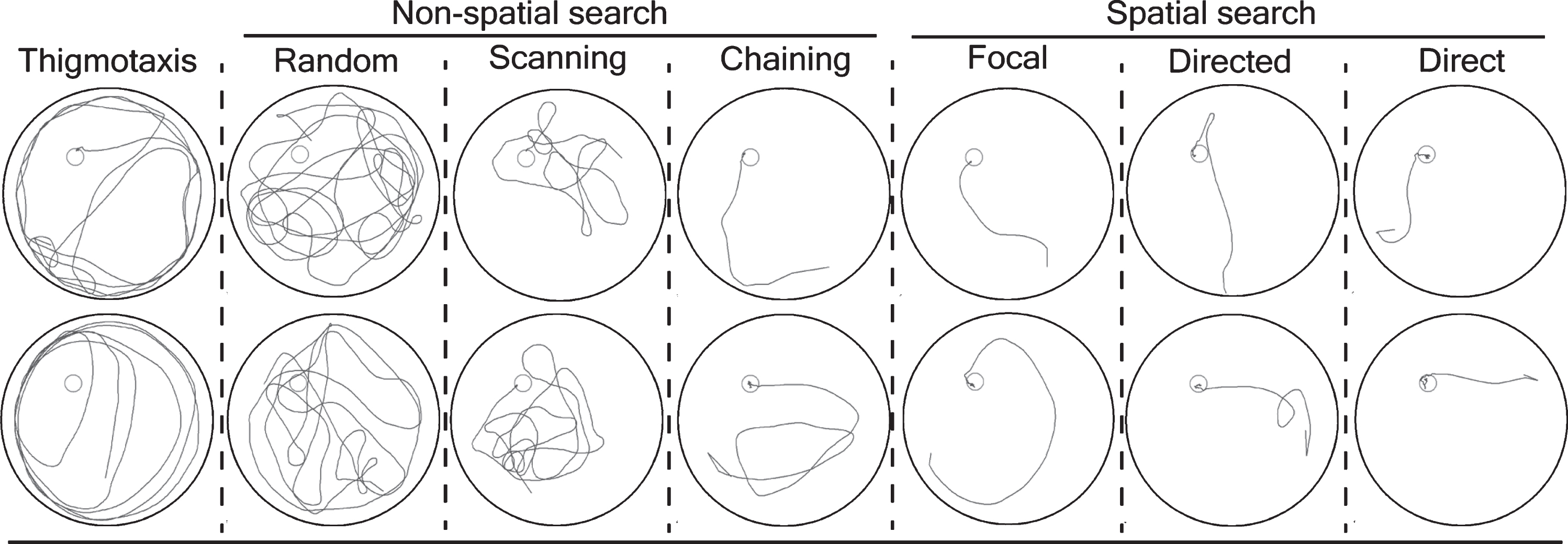
The software automatically classifies each trial into one of the pre-defined search strategies (Fig. 1).
Fig.1
Classification of a mouse trajectory into search strategies. The software algorithm defines the following nine search strategies: thigmotaxis: >35% of time (90 s) within closer wall zone (10 cm from the pool wall) and <65% time in wider wall zone (16 cm from the pool wall); random search: >70% surface coverage; scanning: <70% surface coverage, >15% surface coverage, and <0.7 standardized mean distance to the pool center; chaining: >65% of time within the annulus zone; perseverance: <0.45 standardized error body angle, <0.40 standardized mean distance to the previous goal; directed search: >80% of time in the goal corridor; focal search: <0.35 standardized error body angle, <0.25 standardized mean distance to the present goal; and direct swim: 100% in the goal corridor; unclassified: the algorithm could not classify into above mentioned categories. We further grouped the search strategies into thigmotaxis, non-spatial search strategies (random, scanning, and chaining) and spatial search strategies (focal, directed, and direct). Each column in the figure is a discrete search strategy that consists of two representative mice trajectories (blue lines) from training trials for visualization. The platform is represented by a red circle. Note: The details of key words described can be found in BIOBSERVER water maze manual.
Data analysis and data visualization
The average WM performance was assessed for each mouse per day. The statistical evaluation was performed using a linear mixed model for repeated measures longitudinal data [15, 18] in which proximity is a function of day and group. A day was considered a categorical variable and an animal’s variation was considered a random effect. The statistics were performed using the nlme package in R (v 3.6.1). Similarly, post hoc Tukey’s comparison was performed using the emmeans package in R.
mixed model< - lme (data = WM_training, proximity ∼ group ∗ day, random =∼1|animal)
For probe trials, we also performed a one-way ANOVA analysis using the lm function. Here, a group denotes the group, based on a probe trial.
probe_trial < -1m (data = WM_probe, proximity ∼ group)
All figures were created using either GraphPad Prism software 8.0.1 or ggplot2 package and ggpol [20] in R.
Learning score determination
A learning score system, an extension of the Gallagher learning index [21, 22], was also developed and has been explained in detail before [15]. In brief, the mouse was considered to have learned a task if its average position from the platform (proximity) was 30 cm or less in each of the four-training trials of a given day. When a mouse passed this criterion, a TTC (trials-to-criterion) value was given. For instance, if a mouse passed the criterion for the first time on day 5, it would be awarded a TTC value of 17 as trial no. 17 was the first trial of that day. Then M (multiplier) was determined as a quotient between initialization value (an arbitrary value and in our setup, we have a total of 32 training trials hence we used 33 as initialization value) and TTC. Finally, the learning score of each mouse is the sum product of M and proximity value of a probe trial.
Creation of a spatial intensity map from trail trajectories of the mice
The spatial intensity map of mice trajectories was created from a point pattern map of mice trajectories. A spatial intensity is a function of the spatial location [23]. The point pattern map of mice trajectories was previously applied in similar experiments and details can be found elsewhere [15, 23].
In brief, the mouse trajectory during a WM probe trial was saved as bitmap (bmp) image file (768×629 points) by the Viewer software (Version 3.0, Biobserve GmbH, Bonn, Germany). Next, all images of a specific group were merged at an offset value (0,0) using the pillow library in Python (v3.7.4). The pixel coordinates (x,y) of mice trajectories were later extracted to a csv file using the NumPy library in Python. The point pattern analyses were then conducted using the spatstat package in R (v3.6.1) [24].
A circular frame of observation (radius = 330 units, and center = 330, 315 units) was used to create a window area of 301,982 square units. Now 48,000 pixel coordinates were randomly selected from a csv file and were dumped into a window of observationcovering 78.5% of frame area with an average intensity of 0.14 per square unit. Next, a spatial map was generated using “density” function from randomly selected pixel points using the spatstat package in R [24] that reveals the spatial features. The default Gaussian kernel smoothing was used as an algorithm along with edge correction [23]. The hotspot was visualized with a chosen smoothing sigma parameter (σ= 8).
Principal component analysis (PCA) of WM data-set
PCA is a statistical method that reduces the dimensionality of complex data by geometrically projecting into lower dimensions called principal components (PCs) while maintaining trends and patterns [25]. Here, we also performed PCA on our WM data to reveal the summary of features of cognitive performance. Features, both memory-related and non-memory-related, were carefully selected in a way that all possible features that may affect cognitive performance were covered. Memory-related features included latency, proximity, track-length, Wishaw’s error, heading-angle error, and % target quadrant occupancy. Similarly, non-memory-related features included wall factor and swim-speed. PCA was performed in R (version 3.5.1) and the package FactoMineR [26, 27].
Prediction of the genotype from a phenotype
We used a logistic regression analysis to predict the genotype of a mouse from its phenotype. The phenotypic values were obtained from WM performance features. Features such as latency and proximity were chosen empirically for creating a statistical prediction model. A rule-based approach was used to convert longitudinal data into a single numeric value. First, both proximity and latency data from training trials were used. Next, a rule/criteria was defined which assumes that a mouse learns the task if the proximity value for each trial in a given training day is 30 cm or less or if the latency value is less than 25 s for each trial in a given day. For each mouse, a TTC value was given for both proximity and latency.
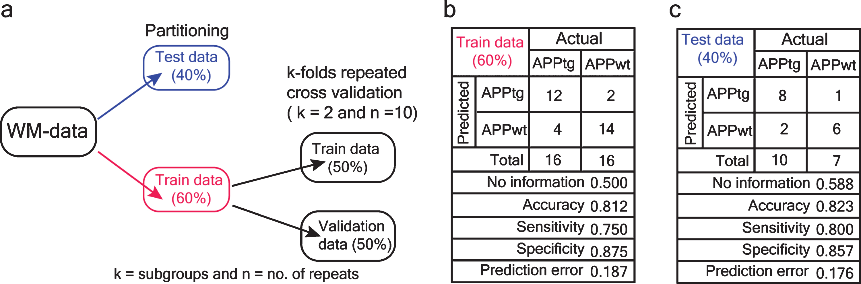
Next, a binomial logistic regression model was applied for 2-category classification as APPtg or APPwt. The numeric data were partitioned into train data and test data (60:40) on a defined random state. To tune the model, the train data were further divided into two subsets (k = 2) in which a model was trained on k-1 of the dataset and then tested on the k-2 dataset. The iteration was repeated ten times. During each iteration, the metrics of the model performance such as sensitivity and specificity were computed. The final average of k-performances’ estimates was assessed. This method of assessing the performance of the model is called k-folds repeated cross-validation [28]. Finally, the model was tested on previously untrained data (test data) for its general applicability. A confusion matrix was computed to assess the prediction generated by the model. Logistic regression, k-folds repeated cross-validation, and confusion matrix were all conducted using the package caret [29] in R.
RESULTS
Inter-trial-interval (ITI) variation affects the spatial learning of APPtg mice
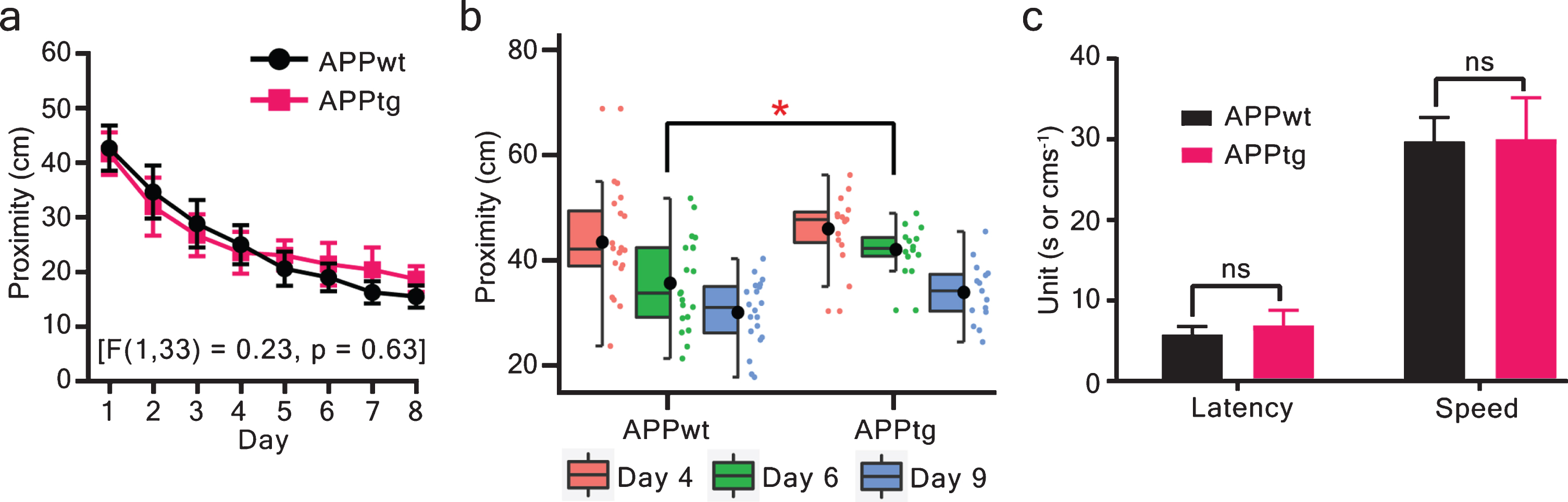
To detect if hippocampal Aβ plaques induced any MCI, we performed the WM task for several days employing protocols with different ITI. First, we completed the WM task for nine consecutive days using long ITI (spaced trials) protocol. Here, APPwt and APPtg mice showed a statistically significant group difference during the probe trial on day 6 (Fig. 2b and Supplementary Figure 3d). However, there was no statistical group difference during training trials or probe trials on day 4 and day 9 (Fig. 2a and Supplementary Figure 3a–c).
Fig.2
MCI was not detected using the long ITI (spaced trials) protocol. Learning and memory were assessed via proximity during training trials and probe trials. a) ANOVA on a mixed model repeated measures did not show any statistically significant group effect. b) Probe trials were conducted on day 4, day 6, and day 9 to assess memory. The proximity values were evaluated and showed that both groups decreased their proximity values as a function of probe trial-day. However, APPwt performed statistically better than APPtg on day 6 (two-tailed unpaired t-test - proximity: p = 0.01. The figure is a half-boxplot with jitter points. A horizontal line is a median, a black circle indicates a mean, a box shows interquartile range (IQR), and the whiskers are 1.5 X IQR. Additionally, individual points are shown as jitter points in a separate vertical column alongside boxplot. c) at the end of the WM task, visual cue trials were conducted to assess visual acuity and motor performance (two-tailed unpaired t-test - latency: p = 0.24; speed: p = 0.94). Values are shown as mean±95% CI (confidence interval). ∗p < 0.05; ns: non-significant; APPwt N = 20 and APPtg N = 15 animals.
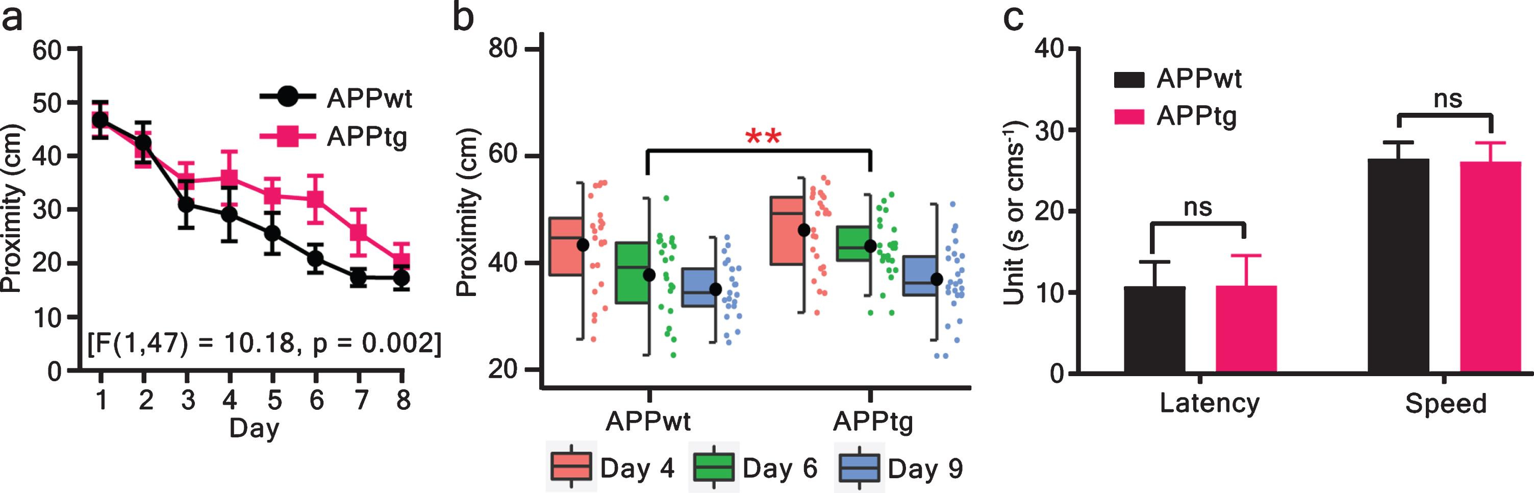
The long-ITI protocol was described to enhance learning in WM task [30]. With the agreement, the long-ITI protocol also did not reveal differences between the groups during training trials (Fig. 2), we shortened the ITI to 1 min (short ITI/massed trials) and trained another cohort of mice for nine consecutive days. Using this protocol, APPwt mice performed significantly better than APPtg mice as revealed by the statistical differences during the probe trial on day 6 (Fig. 3b and Supplementary Figure 4d) as well as during training trials (Fig. 3a and Supplementary Figure 4a–c).
Fig.3
MCI detection of mice using the short-ITI protocol. MCI was assessed via proximity in training trials and probe trials. a) ANOVA of a mixed model repeated measure analysis showed a significant group effect. b) The memory of the platform location was assessed during probe trials. The proximity value decreased gradually from day 4 to day 9 for both groups and showed statistically significant group differences on day 6 (two-tailed unpaired t-test: p = 0.005). Here, a horizontal line is a median, a black circle is a mean, a box is an interquartile range (IQR), and the whiskers are 1.5x IQR. Additionally, individual points are shown as jitter points in a separate vertical column alongside boxplot. c) At the end of the WM task, visual cue trials were conducted to assess visual acuity and motor performance (two-tailed unpaired t-test - latency: p = 0.94; speed: p = 0.76). Values are shown as mean±95% CI (confidence interval). ∗∗p < 0.01; ns: non-significant; APPwt N = 23 and APPtg N = 26 animals.
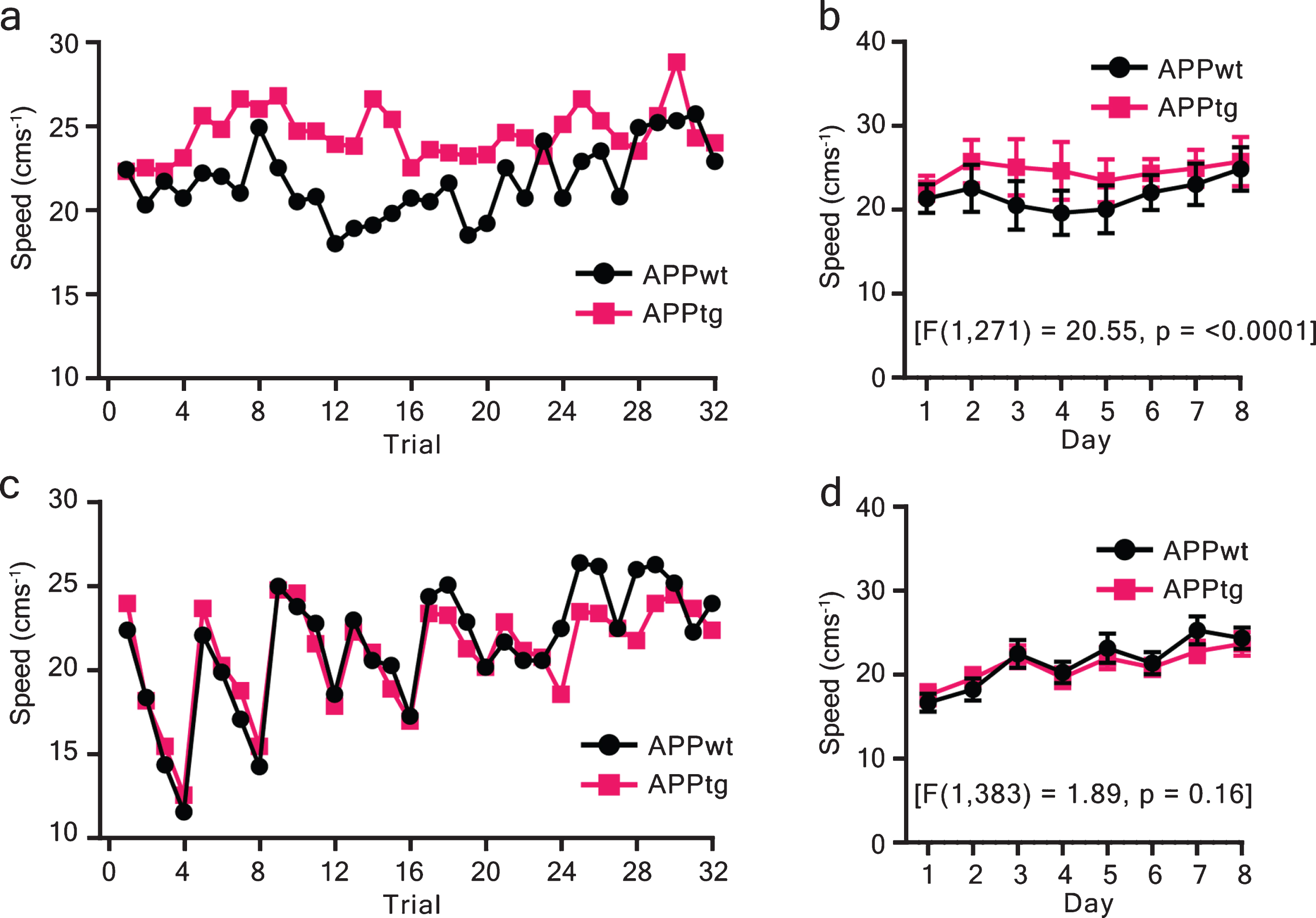
Non-cognitive factors, especially swim-speed, can introduce errors in the cognitive assessment using the WM task. Hence, we investigated swim-speed for both ITI protocols as a function of training trials/days. We found that ITI shortening induced a typical “seesaw” pattern of swim-speed when assessed across training trials (Fig. 4c). Similarly, swim-speed showed a positive trend when assessed across training days (Fig. 4d). Two-way repeated ANOVA between groups did not show any significant difference for short ITI (Fig. 4d), whereas a group difference was detected with long ITI (Fig. 4b).
Fig.4
Swim-speed as a function of training trials/ days. a, b) Speed was assessed across training trials or days for the long-ITI protocol (spaced ITI). c, d) similarly, speed versus training trials (days) were plotted for short-ITI protocol (massed trials). Two-way repeated ANOVA was performed using the lm function in R. The degree of freedom, residual, F-value, and p-value are reported. Values are shown as mean±95% CI (confidence interval).
Next, we performed statistical analysis between all groups during training trials to observe the effect of ITI on the cognitive performance of various groups. We found that shortening the ITI mainly worsened the performance of APPtg mice (Table 2) whereas we did not see any worsening effect on the performance of APPwt mice (Table 2).
Table 2
Summary table showing linear mixed model followed by post hoc Tukey’s comparison on repeated measures data. Proximity was used as a measure of WM performance andvalues were taken from training trials of 3-month-old mice
| Main effect on training trials: [F(3,80) = 14.94, p < 0.0001] | ||||
| Group | estimate | t-ratio | p | |
| 1 | 1-min-ITI APPtg versus 1-min-ITI APPwt | 4.84 | 3.58 | 0.003 |
| 2 | 1-min-ITI APPtg versus 15-min-ITI APPwt | 8.43 | 6.00 | <0.0001 |
| 3 | 1-min-ITI APPtg versus 15-min-ITI APPtg | 7.82 | 5.10 | <0.0001 |
| 4 | 1-min-ITI APPwt versus 15-min-ITI APPwt | 3.59 | 2.48 | 0.06 |
| 5 | 1-min-ITI APPwt versus 15-min-ITI APPtg | 2.97 | 1.89 | 0.23 |
| 6 | 15-min-ITI APPtg versus 15-min-ITI APPwt | 0.61 | 0.38 | 0.98 |
ITI variation does not affect the timeline of the formation of spatial memory
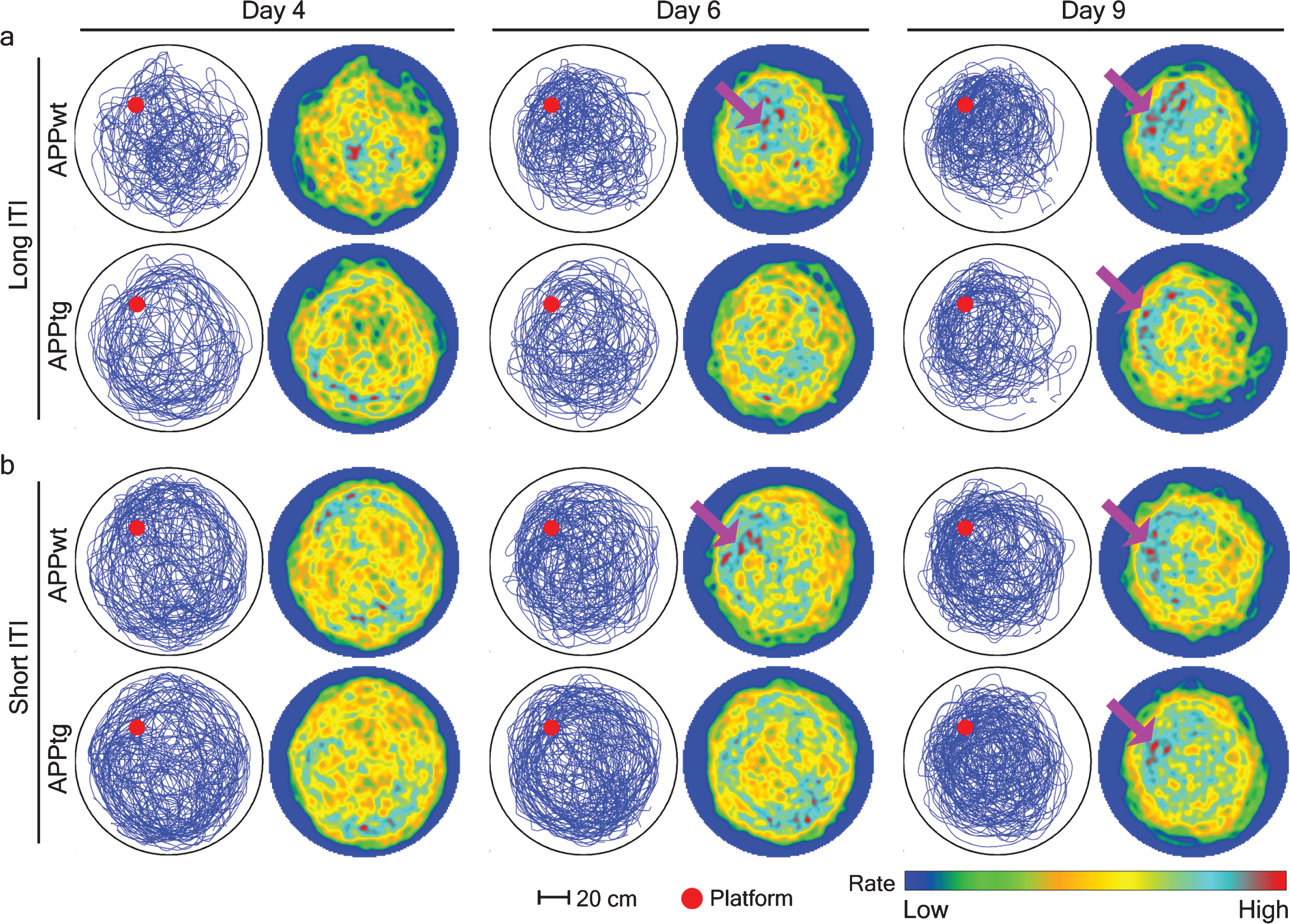
We have demonstrated that increasing ITI promoted spatial learning of APPtg mice (Table 2, row 6) and vice versa (Table 2, row 1). Next, we investigated the role of ITI on the timeline of spatial memory formation. Our protocol included three independent probe trials before normal training trials on different training days. Performing a point pattern analysis of mice trajectories on each probe trial allows us to observe the evolution of spatial memory formation during the WM task. Here, we found that spatial memory formation in both APPwt and APPtg mice was not affected by ITI modulation (Fig. 5). However, we found that spatial memory formation occurred earlier in APPwt (by day 6) as compared with APPtg mice (by day 9) irrespective of ITI (Fig. 5). These results suggest that ITI modulation only affects spatial learning and does not affect the timeline of spatial memory formation inAPPtg.
Fig.5
Spatial intensity estimation of different groups during probe trials in 3-month-old mice. A single probe trial was conducted before normal training trials on day 4, 6, and 9. Mouse trajectories from each group were combined to characterize the location of spatial hotspots. To this aim, the pixel coordinates were extracted from an image and later dropped inside the circular window of observation where Gaussian kernel smoothing was done to create a spatial hotspot. Each row is a group with long or short-ITI protocols. Left, accumulated mice trajectories per group (blue lines) with indicated platform position (red colored circle). Right, color-coded spatial rate map with peak rate (Scale bar). Purple arrows show the location of spatial hotspots.
Learning score as an alternative measure of spatial learning and memory
Since we analyzed spatial learning (training trials) and spatial memory (probe trials) discretely, it is difficult to interpret WM results. Therefore, we amalgamated both training trial and probe trial(s) performance of each mouse into a single numeric value called learning score (LS). Using this approach, we found that the LS of short-ITI APPtg mice was significantly lower than that of other groups (Fig. 6).
Fig.6
Effect of inter-trial-interval in the learning score of 3-month-old mice. The learning score (LS) of each mouse was determined for probe trial 1, probe trials 1 and 2, probe trials 2 and 3, and probe trials 1, 2, and 3, respectively. The LS data were log10 transformed and visualized as violin plot combined with boxplot in which a circular dot (cyan color) represents the mean and the horizontal line inside the boxplot denotes the median. For probe trial(s), a Kruskal-Wallis test was performed on log10 transformed LS data. In case of significant group differences, a post hoc Dunn’s test with Bonferroni correction was performed for multiple pairwise comparisons at alpha level of 0.05. The significant adjusted p-value is denoted alongside the figure. Details: We found a significant group difference for probe trial 1 [χ2(3) = 23.25, p = 0.00003], for probe trials 1 and 2 [χ2(3) = 23.42, p = 0.00003], for probe trials 2 and 3 [χ2(3)=21.96, p = 0.00006], and for probe trials 1,2, and 3 [χ2(3) = 23.41, p = 0.00003]. No. of animals per group: Long-ITI APPwt N = 20, Long-ITI APPtg N = 15 Short-ITI APPwt N = 23, Short-ITI APPtg N = 26. p is adjusted p-value and χ2 is chi-squared. ∗p < 0.05; ∗∗p < 0.01; ∗∗∗p < 0.001; ∗∗∗∗p < 0.0001.
![Effect of inter-trial-interval in the learning score of 3-month-old mice. The learning score (LS) of each mouse was determined for probe trial 1, probe trials 1 and 2, probe trials 2 and 3, and probe trials 1, 2, and 3, respectively. The LS data were log10 transformed and visualized as violin plot combined with boxplot in which a circular dot (cyan color) represents the mean and the horizontal line inside the boxplot denotes the median. For probe trial(s), a Kruskal-Wallis test was performed on log10 transformed LS data. In case of significant group differences, a post hoc Dunn’s test with Bonferroni correction was performed for multiple pairwise comparisons at alpha level of 0.05. The significant adjusted p-value is denoted alongside the figure. Details: We found a significant group difference for probe trial 1 [χ2(3) = 23.25, p = 0.00003], for probe trials 1 and 2 [χ2(3) = 23.42, p = 0.00003], for probe trials 2 and 3 [χ2(3)=21.96, p = 0.00006], and for probe trials 1,2, and 3 [χ2(3) = 23.41, p = 0.00003]. No. of animals per group: Long-ITI APPwt N = 20, Long-ITI APPtg N = 15 Short-ITI APPwt N = 23, Short-ITI APPtg N = 26. p is adjusted p-value and χ2 is chi-squared. ∗p < 0.05; ∗∗p < 0.01; ∗∗∗p < 0.001; ∗∗∗∗p < 0.0001.](https://content.iospress.com:443/media/jad/2020/77-3/jad-77-3-jad200675/jad-77-jad200675-g006.jpg)
Thigmotaxis is inversely associated with ITI duration
To find out how MCI in APPtg mice could only be detected in the short-ITI protocol, we analyzed the evolution of search strategies as a function of training days in the different ITI protocols. We found that non-spatial search (chaining, scanning, and random) dominated in both short ITI as well as in long ITI (Fig. 7). Interestingly, thigmotaxis was more pronounced for both APPwt and APPtg mice upon shortening of ITI(Fig. 8).
Fig.7
Search strategies of mice in different protocols in the WM task. Search strategies were qualitatively classified into thigmotaxis, non-spatial search, and spatial search. Non-spatial search strategies included unclassified, random, scanning, and chaining. Spatial strategies included direct, directed and focal search. Search strategy for each trial was determined as described above (refer to “Methods section: Video analysis and search classification”).
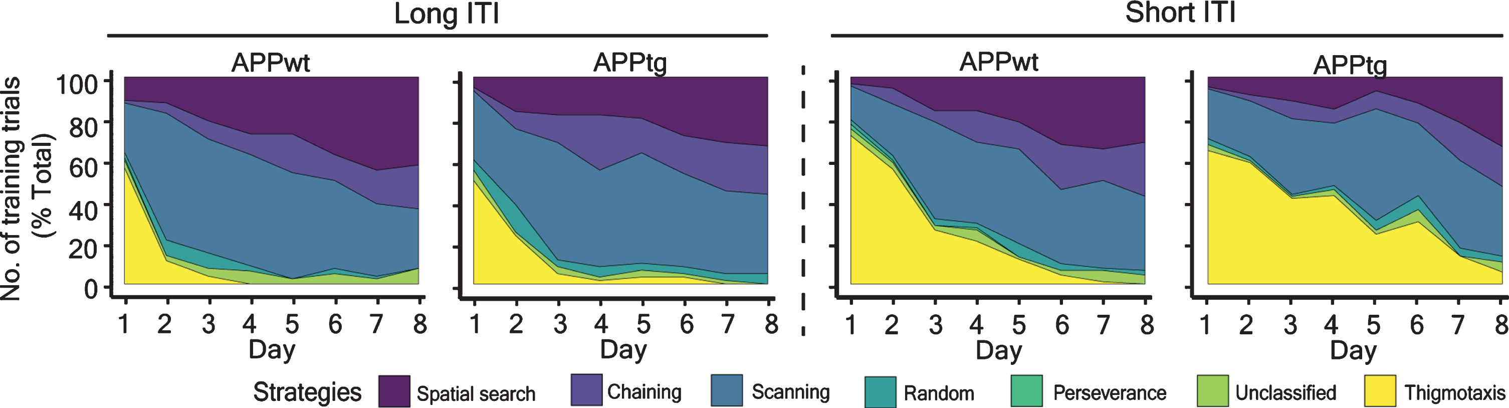
Fig.8
Logistic regression of WM data. a) The WM data were randomly divided into training (60%) and test dataset (40%) The training dataset was further divided into training and validation dataset as two subsets. Next, k-folds repeated cross-validation was performed. b) Average values of various metrics of model evaluation on train data set. c) Model evaluation on previously untrained dataset (test data).
Consequently, we aimed to investigate the contribution of thigmotaxis in the short-ITI protocol. Selected features were extracted from the WM-dataset and principal component analysis (PCA) was performed. First, the combined contribution of principal component 1 (PC1) and principal component 2 (PC2) accounted for more than 80% of the variance for both the combined and separate group analyses (Table 3). Second, neither the wall factor nor the swim-speed was dominant in PC1 (Table 3). Third, our data indicates that WM performance in the WM task was a combined effect of multiple variables such as latency, proximity, track length, wall factor (thigmotaxis), etc.
Table 3
Principal component analysis (PCA) of various features in the short-ITI protocol. From a combined dataset of 1,566 trials (APPwt and APPtg animals), about 72% of the behavioral variability was contributed by PC1. Similar results were obtained for APPwt and APPtg mice. PC1 is principalcomponent 1 and PC2 is principal component 2
| APPwt and APPtg | APPwt | APPtg | ||||
| (1566 trials) | (736 trials) | (830 trials) | ||||
| Features | PC1 | PC2 | PC1 | PC2 | PC1 | PC2 |
| Latency | 16.18 | 1.39 | 15.97 | 1.10 | 16.41 | 1.26 |
| Proximity | 16.71 | 0.005 | 16.58 | 0.03 | 16.87 | 0.0005 |
| Track length | 14.01 | 2.68 | 13.91 | 0.54 | 14.13 | 4.86 |
| Wall factor | 13.45 | 0.14 | 13.15 | 0.002 | 13.65 | 0.17 |
| Wishaw’s error | 16.08 | 0.93 | 15.88 | 1.05 | 16.29 | 0.95 |
| % target quadrant occupancy | 15.40 | 0.01 | 15.29 | 0.09 | 15.48 | 0.006 |
| Swim-speed | 5.90 | 1.11 | 6.51 | 1.28 | 5.37 | 7.25 |
| Heading-angle error | 2.22 | 93.70 | 2.67 | 95.88 | 1.77 | 85.47 |
| Variance | 5.75 | 0.90 | 5.81 | 0.87 | 5.69 | 0.94 |
| % Variance | 71.97 | 11.29 | 72.63 | 10.94 | 71.18 | 11.77 |
Genotype can be reliably predicted
The PCA analysis suggested that WM performance might be affected by a combination of multiple features. To test this hypothesis, we chose popular learning variables, latency and proximity, and created a simple statistical model based on the logistic regression algorithm to predict the binary classification of mice as either APPtg or APPwt. Here, we randomly trained our model on the WM-data set. Additionally, k-folds repeated cross-validation was performed on a training dataset (Fig. 8b). Finally, we evaluated the model on a previously untrained dataset (test data) and showed that the genotype of a mouse can be predicted with 82.3 % accuracy and 80% sensitivity (Fig. 8c).
DISCUSSION
Cognitive decline is a defining symptom of AD and mouse models have been generated to recapitulate different aspects of cognitive changes observed in AD patients. However, an enormous heterogeneity has been observed between the time course and the progression of cognitive change across different AD mouse models [31]. Foley and colleagues performed a systematic review of different AD mouse models and found no statistically significant correlation between quantified Aβ levels and the early cognitive decline/mild cognitive impairment [32]. They surmise that the quantified Aβ levels were not “high” enough to detect the cognitive change [32]. The present study aimed to identify early cognitive changes in an AD mouse model, specifically APPPS1-21 mice. To attain this goal, we performed a WM task using different ITI versions of our protocol, compared with wild-type littermates, and showed that MCI can be detected simultaneously when Aβ plaques start to appear in the hippocampus. However, we did not provide the immunohistochemistry of Aβ plagues on the hippocampus in this study. There are two main reasons: First, this mouse model has been thoroughly characterized previously by Radde and colleagues. They assessed the spatiotemporal progression of Aβ production from early age using immunohistochemistry and found out that the Aβ plaques in hippocampus region appear from 3 months of age [6]. And second, our group has also been using this specific mouse model for more than a decade and found consistently that Aβ plaques indeed start to appear in hippocampus from 3 months of age [10].
The detection of MCI is important because the clinical benefit of treatment seems unachievable when the disease is already progressed in the late stage of AD [33, 34]. Several agents have been tested for AD to modify the disease progression without any success [35]. Hence, understanding early stage of AD such as MCI is vital not only for preventing the deterioration of AD pathogenesis but also for finding potential treatment strategies. Since the WM task is a popular test of spatial learning and memory, we investigated different ways of detection and visualization of MCI using this task. Consequently, we provided additional approaches to MCI visualization such as a spatial learning index (Fig. 6) and the spatial intensity map (Fig. 5). This study not only focuses on the detection but also the prediction of MCI with the intention of drug screening. To achieve this goal, one avenue can be the use of classification algorithms such as decision trees, logistic regression, random forest algorithms etc. to predict the genotype of a mouse. To implement classification algorithms, the complex behavior of a mouse should be reduced into a single number system. However, there are two main difficulties: First, the WM-data is a longitudinal time-series data in which the subsequent trial is affected by the performance of the previous trial [18]. Second, multiple variables (latency, track-length, proximity) have been used to describe spatial cognition [11, 30].
The problem of longitudinal data can be solved by converting the WM-data into a single numeric value. Historically, Gallagher et al. [21] developed a learning index/score as a new measure of spatial learning for group comparison. This approach amalgamated the time-series data into a single numeric value. The idea of converting WM-data into single number has been used by others as well [36]. In this study, we also reduced all training trials into a single number so that classification algorithms can be easily applied. Similarly, we performed PCA analysis to solve the second problem. PCA is a statistical procedure to determine the important contributing features in a given dataset. Studies have shown that performance in a WM task can be modulated by multiple factors [17, 30, 37–39]. Here, using PCA, we also determined the most contributing features of training trials (Table 3).
Finally, we used a simple logistic regression algorithm as a tool for predictive analysis of a mouse into APPtg or APPwt. Because of small animal size (total 49 mice), some animals had to be included in this study from a previous study (9 APPwt and 10 APPtg were also included in this data analysis from Set-up I experiment [15]). Again, we used repeated k-folds cross-validation on training datasets to handle small datasets. In this approach, the training data will be randomly partitioned into training and validation datasets and the average performance-matrices such as sensitivity and specificity were assessed from the n-th iteration. The simple binary logistic regression algorithm later predicted APPtg and APPwt with high-performance matrices (Fig. 8c), especially considering the relatively low amount of input data. Such an approach can be further extended to test the pharmacological effect of a putative cognitive enhancer, anti-Alzheimer’s drug, etc., as misclassification of APPtg as APPwt will be increased in case of true positive effects.
Our study provided important new insights into spatial learning and spatial memory. We investigated the MCI detection and visualization using different ITI protocols. To detect MCI, we used two different ITI protocols: 1) Long ITI (spaced trials or 15–40 min ITI) and 2) short ITI (massed trials or 1 min ITI). We expected that mice, irrespective of its transgene, tested in short ITI should perform poorly as compared to long ITI [40]. However, a shortening of ITI only worsened the spatial learning of APPtg but not APPwt mice (Table 2). More interestingly, ITI variation does not alter the formation of spatial memory in APPtg mice and APPwt mice (Fig. 5). Spatial memory forms earlier in APPwt than APPtg mice (Figs. 2, 3, and 5) suggesting that spatial learning can be modulated by ITI, but the spatial memory formation cannot be modulated by the ITI changes in APPtg.
Earlier studies have been performed to reveal the causality of ITI modulation on the cognitive difference between groups. Prolonging ITI promotes learning whereas shortening ITI decreases spatial learning [40, 41]. Kogan and colleagues performed a WM task in CREBαΔ - mutant mice and found out that increasing ITI from 1 min to 60 min completely removed the spatial memory deficit in these mutant mice [41]. It was initially surmised that stress and/or fatigue could be a causal factor in the learning difference observed in short-ITI protocol [42]. Later, it was shown that cold water (19°C) significantly increased circulating corticosterone level in rats [43]. Additionally, Iivonen and colleagues reported that swimming in water (20°C) for 45 s for five trials with ITI of 30 s significantly dropped rectal body temperature in mice. The hypothermia was then accompanied by decreasing swim-speed. We, therefore, assessed swim-speed in this study and found a similar pattern of slowing of swim-speed as a function of training trials for a day during early training trials (Fig. 4c). However, the “slowing of swim-speed” does not explain the rationality behind the short ITI and the cognitive difference between groups.
One of the least understood aspects in the field of learning and memory is the spacing effect [45] where increasing the ITI between two successive trial is beneficial for memory [46]. This spacing effect has been observed in diverse memory tasks in humans [47] as well as non-humans [45]. However, the key mechanism of underlying superiority of spaced training (long ITI) over massed training (short ITI) has not been understood [45]. Few studies have been performed to unravel the synaptic evidence for the efficacy of spaced training. Kramár and colleagues performed theta bursts stimulation (TBS) experiment on hippocampal slices to study long term potentiation (LTP), a key mechanism in learning and memory [16], and showed that TBS with longer delays produces a greater degree of LTP as compared to shorter delays [48].
There are several limitations to this study. First, we have only used female mice and have not studied gender-specific performances. Female-specific increased risk in AD is related to inherent biological differences such as sex-specific gene-interaction, hormonal changes as a function of aging, and sexual dimorphism in brain structures [49]. Second, mouse models of AD do not completely reflect the full spectrum of human cognitive dysfunction. Moreover, transgenic animal models can produce several artifacts due to artificial transgene overexpression [50]. Despite these limitations, behavioral studies in mice can give important information regarding the cognitive dysfunction and pathogenesis of AD [51].
This study unraveled early cognitive difference in an AD mouse model via multiple approaches such as experimental modulation as well as alternative approaches of analyzing the complex data of WM tasks such as learning score and classification algorithm. Detecting MCI at a young age will open new avenues of potential treatment strategies such as treatment at a younger age and faster drug screening.
ACKNOWLEDGMENTS
This work was supported by: Deutsche Forschungsgemeinschaft/ Germany (DFG PA930/12); Ministerium für Wirtschaft und Wissenschaft Sachsen-Anhalt/ Germany (ZS/2016/05/78617); Leibniz Gemeinschaft/ Germany (SAW-2015-IPB-2); Latvian Council of Science/ Latvia (lzp-2018/1-0275); Nasjonalforeningen for folkehelse (16154), HelseSØ/ Norway (2016062, 2019054, 2019055); Norges forskningsrådet/ Norway (251290, 260786); European Commission (643417).
We would like to thank Ivan Eiriz and Thomas Brüning for technical support.
Authors’ disclosures available online (https://www.j-alz.com/manuscript-disclosures/20-0675r1).
SUPPLEMENTARY MATERIAL
[1] The supplementary material is available in the electronic version of this article: https://dx.doi.org/10.3233/JAD-200675.
REFERENCES
[1] | Geda YE , Schneider LS , Gitlin LN , Miller DS , Smith GS , Bell J , Evans J , Lee M , Porsteinsson A , Lanctot KL , Rosenberg PB , Sultzer DL , Francis PT , Brodaty H , Padala PP , Onyike CU , Ortiz LA , Ancoli-Israel S , Bliwise DL , Martin JL , Vitiello MV , Yaffe K , Zee PC , Herrmann N , Sweet RA , Ballard C , Khin NA , Alfaro C , Murray PS , Schultz S , Lyketsos CG , Neuropsychiatric Syndromes Professional Interest Area of ISTAART ((2013) ) Neuropsychiatric symptoms in Alzheimer’s disease: Past progress and anticipation of the future. Alzheimers Dement 9: , 602–608. |
[2] | Bowen J , Teri L , Kukull W , McCormick W , McCurry SM , Larson EB ((1997) ) Progression to dementia in patients with isolated memory loss. Lancet 349: , 763–765. |
[3] | Petersen RC , Doody R , Kurz A , Mohs RC , Morris JC , Rabins PV , Ritchie K , Rossor M , Thal L , Winblad B ((2001) ) Current concepts in mild cognitive impairment. Arch Neurol 58: , 1985–1992. |
[4] | Albert MS , DeKosky ST , Dickson D , Dubois B , Feldman HH , Fox NC , Gamst A , Holtzman DM , Jagust WJ , Petersen RC , Snyder PJ , Carrillo MC , Thies B , Phelps CH ((2011) ) The diagnosis of mild cognitive impairment due to Alzheimer’s disease: Recommendations from the National Institute on Aging-Alzheimer’s Association workgroups on diagnostic guidelines for Alzheimer’s disease. Alzheimers Dement 7: , 270–279. |
[5] | Pepeu G ((2004) ) Mild cognitive impairment: Animal models. Dialogues Clin Neurosci 6: , 369–377. |
[6] | Radde R , Bolmont T , Kaeser SA , Coomaraswamy J , Lindau D , Stoltze L , Calhoun ME , Jaggi F , Wolburg H , Gengler S , Haass C , Ghetti B , Czech C , Holscher C , Mathews PM , Jucker M ((2006) ) Abeta42-driven cerebral amyloidosis in transgenic mice reveals early and robust pathology. EMBO Rep 7: , 940–946. |
[7] | Scheffler K , Stenzel J , Krohn M , Lange C , Hofrichter J , Schumacher T , Bruning T , Plath AS , Walker L , Pahnke J ((2011) ) Determination of spatial and temporal distribution of microglia by 230nm-high-resolution, high-throughput automated analysis reveals different amyloid plaque populations in an APP/PS1 mouse model of Alzheimer’s disease. Curr Alzheimer Res 8: , 781–788. |
[8] | Krohn M , Lange C , Hofrichter J , Scheffler K , Stenzel J , Steffen J , Schumacher T , Bruning T , Plath AS , Alfen F , Schmidt A , Winter F , Rateitschak K , Wree A , Gsponer J , Walker LC , Pahnke J ((2011) ) Cerebral amyloid-beta proteostasis is regulated by the membrane transport protein ABCC1 in mice. J Clin Invest 121: , 3924–3931. |
[9] | Frohlich C , Paarmann K , Steffen J , Stenzel J , Krohn M , Heinze HJ , Pahnke J ((2013) ) Genomic background-related activation of microglia and reduced beta-amyloidosis in a mouse model of Alzheimer’s disease. Eur J Microbiol Immunol (Bp) 3: , 21–27. |
[10] | Paarmann K , Prakash SR , Krohn M , Mohle L , Brackhan M , Bruning T , Eiriz I , Pahnke J ((2019) ) French maritime pine bark treatment decelerates plaque development and improves spatial memory in Alzheimer’s disease mice. Phytomedicine 57: , 39–48. |
[11] | Morris RG , Garrud P , Rawlins JN , O’Keefe J ((1982) ) Place navigation impaired in rats with hippocampal lesions. Nature 297: , 681–683. |
[12] | Milner B ((1972) ) Disorders of learning and memory after temporal lobe lesions in man. Clin Neurosurg 19: , 421–446. |
[13] | Squire LR ((1992) ) Memory and the hippocampus: A synthesis from findings with rats, monkeys, and humans. Psychol Rev 99: , 195–231. |
[14] | Serneels L , Van Biervliet J , Craessaerts K , Dejaegere T , Horre K , Van Houtvin T , Esselmann H , Paul S , Schafer MK , Berezovska O , Hyman BT , Sprangers B , Sciot R , Moons L , Jucker M , Yang Z , May PC , Karran E , Wiltfang J , D’Hooge R , De Strooper B ((2009) ) gamma-Secretase heterogeneity in the Aph1 subunit: Relevance for Alzheimer’s disease. Science 324: , 639–642. |
[15] | Rai SP , Krohn M , Pahnke J ((2020) ) Early cognitive training rescues remote spatial memory but reduces cognitive flexibility in Alzheimer’s disease mice. J Alzheimers Dis 75: , 1301–1317. |
[16] | Morris RG , Moser EI , Riedel G , Martin SJ , Sandin J , Day M , O’Carroll C ((2003) ) Elements of a neurobiological theory of the hippocampus: The role of activity-dependent synaptic plasticity in memory. Philos Trans R Soc Lond B Biol Sci 358: , 773–786. |
[17] | D’Hooge R , De Deyn PP ((2001) ) Applications of the Morris water maze in the study of learning and memory. Brain Res Brain Res Rev 36: , 60–90. |
[18] | Young ME , Clark MH , Goffus A , Hoane MR ((2009) ) Mixed effects modeling of Morris water maze data: Advantages and cautionary notes. Learn Motiv 40: , 160–177. |
[19] | Wickham H ((2011) ) ggplot2. Wiley Interdiscip Rev Comput Stat 3: , 180–185. |
[20] | Tiedemann F ((2020) ) Visualizing Social Science Data with ‘ggplot2‘. https://github.com/erocoar/ggpol. |
[21] | Gallagher M , Burwell R , Burchinal M ((2015) ) Severity of spatial learning impairment in aging: Development of a learning index for performance in the Morris water maze. Behav Neurosci 129: , 540–548. |
[22] | Tomas Pereira I , Burwell RD ((2015) ) Using the spatial learning index to evaluate performance on the water maze. Behav Neurosci 129: , 533–539. |
[23] | Baddeley A , Rubak E , Turner R ((2015) ) Spatial point patterns: Methodology and applications with R, Chapman and Hall/CRC. |
[24] | Baddeley A , Turner R ((2005) ) spatstat: AnRPackage for analyzing spatial point patterns. J Stat Softw 12: , 10.18637/jss.v012.i06. |
[25] | Lever J , Krzywinski M , Altman N ((2017) ) Points of significance: Principal component analysis. Nature Publishing Group. |
[26] | Catuara-Solarz S , Espinosa-Carrasco J , Erb I , Langohr K , Notredame C , Gonzalez JR , Dierssen M ((2015) ) Principal component analysis of the effects of environmental enrichment and (-)-epigallocatechin-3-gallate on age-associated learning deficits in a mouse model of Down syndrome. Front Behav Neurosci 9: , 330. |
[27] | Lê S , Josse J , Husson F ((2008) ) FactoMineR: AnRPackage for multivariate analysis. J Stat Softw 25: , 1–18. |
[28] | Dasgupta A , Sun YV , Konig IR , Bailey-Wilson JE , Malley JD ((2011) ) Brief review of regression-based and machine learning methods in genetic epidemiology: The Genetic Analysis Workshop 17 experience. Genet Epidemiol 35: (Suppl 1), S5–11. |
[29] | Kuhn M ((2008) ) Building predictive models in R using the caret package. J Stat Softw 28: , 1–26. |
[30] | Vorhees CV , Williams MT ((2006) ) Morris water maze: Procedures for assessing spatial and related forms of learning and memory. Nat Protoc 1: , 848–858. |
[31] | Webster SJ , Bachstetter AD , Nelson PT , Schmitt FA , Van Eldik LJ ((2014) ) Using mice to model Alzheimer’s dementia: An overview of the clinical disease and the preclinical behavioral changes in 10 mouse models. Front Genet 5: , 88. |
[32] | Foley AM , Ammar ZM , Lee RH , Mitchell CS ((2015) ) Systematic review of the relationship between amyloid-β levels and measures of transgenic mouse cognitive deficit in Alzheimer’s disease. J Alzheimers Dis 44: , 787–795. |
[33] | Counts SE , Ikonomovic MD , Mercado N , Vega IE , Mufson EJ ((2017) ) Biomarkers for the early detection and progression of Alzheimer’s disease. Neurotherapeutics 14: , 35–53. |
[34] | Sasaguri H , Nilsson P , Hashimoto S , Nagata K , Saito T , De Strooper B , Hardy J , Vassar R , Winblad B , Saido TC ((2017) ) APP mouse models for Alzheimer’s disease preclinical studies. EMBO J 36: , 2473–2487. |
[35] | Graham WV , Bonito-Oliva A , Sakmar TP ((2017) ) Update on Alzheimer’s disease therapy and prevention strategies. Annu Rev Med 68: , 413–430. |
[36] | Chen G , Chen KS , Knox J , Inglis J , Bernard A , Martin SJ , Justice A , McConlogue L , Games D , Freedman SB , Morris RG ((2000) ) A learning deficit related to age and beta-amyloid plaques in a mouse model of Alzheimer’s disease. Nature 408: , 975–979. |
[37] | Gulinello M , Gertner M , Mendoza G , Schoenfeld BP , Oddo S , LaFerla F , Choi CH , McBride SM , Faber DS ((2009) ) Validation of a 2-day water maze protocol in mice. Behav Brain Res 196: , 220–227. |
[38] | Ruediger S , Spirig D , Donato F , Caroni P ((2012) ) Goal-oriented searching mediated by ventral hippocampus early in trial-and-error learning. Nat Neurosci 15: , 1563–1571. |
[39] | Morris R ((1984) ) Developments of a water-maze procedure for studying spatial learning in the rat. J Neurosci Methods 11: , 47–60. |
[40] | Upchurch M , Wehner JM ((1990) ) Effects of N-methyl-D-aspartate antagonism on spatial learning in mice. Psychopharmacology (Berl) 100: , 209–214. |
[41] | Kogan JH , Frankland PW , Blendy JA , Coblentz J , Marowitz Z , Schütz G , Silva AJ ((1997) ) Spaced training induces normal long-term memory in CREB mutant mice. Curr Biol 7: , 1–11. |
[42] | Rick JT , Murphy MP , Ivy GO , Milgram NW ((1996) ) Short intertrial intervals impair water maze performance in old Fischer 344 rats. J Gerontol A Biol Sci Med Sci 51: , B253–260. |
[43] | Akirav I , Kozenicky M , Tal D , Sandi C , Venero C , Richter-Levin G ((2004) ) A facilitative role for corticosterone in the acquisition of a spatial task under moderate stress. Learn Mem 11: , 188–195. |
[44] | Iivonen H , Nurminen L , Harri M , Tanila H , Puolivali J ((2003) ) Hypothermia in mice tested in Morris water maze. Behav Brain Res 141: , 207–213. |
[45] | Smolen P , Zhang Y , Byrne JH ((2016) ) The right time to learn: Mechanisms and optimization of spaced learning. Nat Rev Neurosci 17: , 77–88. |
[46] | Toppino TC , Gerbier E ((2014) ) About practice: Repetition, spacing, and abstraction. In Psychology of learning and motivation. Elsevier, pp. 113–189. |
[47] | Cepeda NJ , Pashler H , Vul E , Wixted JT , Rohrer D ((2006) ) Distributed practice in verbal recall tasks: A review and quantitative synthesis. Psychol Bull 132: , 354–380. |
[48] | Kramár EA , Babayan AH , Gavin CF , Cox CD , Jafari M , Gall CM , Rumbaugh G , Lynch G ((2012) ) Synaptic evidence for the efficacy of spaced learning. Proc Natl Acad Sci U S A 109: , 5121–5126. |
[49] | Fisher DW , Bennett DA , Dong H ((2018) ) Sexual dimorphism in predisposition to Alzheimer’s disease. Neurobiol Aging 70: , 308–324. |
[50] | Jankowsky JL , Zheng H ((2017) ) Practical considerations for choosing a mouse model of Alzheimer’s disease. Mol Neurodegener 12: , 89. |
[51] | Onos KD , Sukoff Rizzo SJ , Howell GR , Sasner M ((2016) ) Toward more predictive genetic mouse models of Alzheimer’s disease. Brain Res Bull 122: , 1–11. |


