Shape-Attributes of Brain Structures as Biomarkers for Alzheimer’s Disease
Abstract
We describe a fully automatic framework for classification of two types of dementia based on the differences in the shape of brain structures. We consider Alzheimer’s disease (AD), mild cognitive impairment of individuals who converted to AD within 18 months (MCIc), and normal controls (NC). Our approach uses statistical learning and a feature space consisting of projection-based shape descriptors, allowing for canonical representation of brain regions. Our framework automatically identifies the structures most affected by the disease. We evaluate our results by comparing to other methods using a standardized data set of 375 adults available from the Alzheimer’s Disease Neuroimaging Initiative (ADNI). Our framework is sensitive to identifying the onset of Alzheimer’s disease, achieving up to 88.13% accuracy in classifying MCIc versus NC, outperforming previous methods.
INTRODUCTION
Alzheimer’s disease (AD) is a progressive, degenerative brain disease and is the most common form of dementia in adults aged 65 and older. Worldwide prevalence of AD is expected to rise to over 100 million by 2050 [1]. Many studies provide evidence suggesting that AD progresses by selective degeneration of neuronal populations in several brain regions. The hippocampus is one of the earliest structures to be affected [2]. Mild cognitive impairment (MCI) is a prodromal stage of AD with a conversion rate of about 10% [3]. Studying why only certain individuals with MCI develop AD is fundamental to understanding the diseases and developing accurate prognostic indicators.
Magnetic resonance imaging (MRI) of AD patients reveals overall volume loss and shape changes in specific brain structures, such as the hippocampus, amygdala, corpus callosum, and other regions [4]. Fig. 1 shows a comparison of coronal and axial views of T1-weighted MR scans: a healthy 79-year-old female on the left, and a 74-year-old female diagnosed with AD on the right. The left hippocampi and lateral ventricles are shown in detail on the side panels. An overall tissue loss is apparent in the late-stage AD patient. As neurons die, the brain parenchyma shrinks, leading to passive enlargement of the brain ventricles. The purpose of this work is to explore the subtle changes in shape of brain structures most affected by AD. We develop shape descriptors to capture and quantify these changes, and test their efficacy as imaging biomarkers for automatic classification of the following populations: MCI patients who progressed to AD, AD patients, and normal controls (NC). We are using a novel 3D shape descriptor, combining information from an ensemble of brain structures and employing machine learning. We evaluate our framework on a cohort of 375 subjects available through the Alzheimer’s Disease Neuroimaging Initiative (ADNI), compare our results to other methods, and perform an analysis of the significance of the different features we extract.
MATERIALS AND METHODS
Data
Data used in the preparation of this article were obtained from the ADNI database (http://adni.loni.usc.edu) [5]. The ADNI was launched in 2003 as a public-private partnership, led by Principal Investigator Michael W. Weiner, MD. The primary goal of ADNI has been to test whether serial MRI, positron emission tomography (PET), other biological markers, and clinical and neuropsychological assessment can be combined to measure the progression of MCI and early AD). For up-to-date information, see http://www.adni-info.org. For comparison to other methods, we used the same dataset as reported in [6] for three groups of subjects: 162 cognitively normal elderly controls (CN), 137 patients with AD, and 76 patients with MCI who had converted to AD within 18 months (MCIc). Demographic characteristics of the studied population can be found in [6]. Details about data pre-processing can be found in [5].
Processing framework overview
The main contribution of this work is a computational framework that performs automatic classification between different types of dementia, namely MCIc and AD. We achieve top performance in identifying the MCI patients that will convert to Alzheimer’s within 18 months (MCIc). This section is an overview of the processing steps. Details about each step can be found in following subsections.
The inputs to our framework are the T1-weighted MR images preprocessed with the Freesurfer image analysis suite, freely available at http://freesurfer.net [7]. Freesurfer outputs a 3D segmentation of 115 cortical and subcortical brain structures according to the Desikan-Killiany Atlas [8]. A subset of 8 regions of interest (ROIs) (see below) is chosen and processed separately: first, a projection of the ROI on its principal plane is calculated (see Projections for details). 2D shape descriptors are calculated for each ROI, resulting in only 6 values per ROI (see Shape descriptor calculation for details). We then construct a 32-long feature vector for each subject by concatenating the feature values from all ROIs. These steps are repeated for all subjects in the dataset.
Following this processing, the dataset is split in half: 50% used for training the classifier, and the rest is used for test and evaluation. To find the optimal training parameters, we performed 5-fold cross validation on the training set (see SVM Classication for details). Finally, we test our model on the independent testing set, evaluate its performance and compare to other methods (see Comparison to other methods for details). Additionally, in order to understand the importance of each brain structure and its derived features for the classification, we perform feature analysis experiments (see Feature analysis experiments for details).
Data preprocessing and ROI extraction
It is commonly accepted that at progressive stages of AD, degeneration of brain tissue occurs, leading to structural changes in several brain structures (see [4] for a list of supporting research), including the hippocampi and the ventricles [9]. In this work we focus on a subset of these structures and choose the following ROIs:
1. The hippocampi (left and right)
2. Inferior lateral ventricles (left and right)
3. 3rd Ventricle
4. Right lateral ventricle
5. Cerebral white matter (left and right)2
Each ROI is a volumetric shape represented as a set of points
Projections
We use projections to reduce the dimensionality of the data. For each ROI, we first find the principal axes of the 3D shape using the NIPALS algorithm for principal component analysis (PCA) [10]. We project each ROI onto the plane spanned by the first two principal components. Then, to calculate the projection, we first partition the 2D plane into H × W bins, where the values of H and W are of the order of 20 to 40 pixels, unique for each ROI type, but kept the same (normalized) across all subjects for the specific ROI. The value of each pixel f (i, j) on the H × W projection matrix is obtained by counting how many points
(1)
Shape descriptor calculation
We encode the information of the 2D projection image in a compact feature descriptor. In this work we focused on moments [11] and entropy. Moments have been widely used in statistics to describe the shape of a probability density function, in computer vision to describe the shape of objects, e.g., [12] and in classic rigid-body mechanics to describe the distribution of mass in a body. The equation for central moment of order p + q is
(2)
where f (i, j) is the image intensity at location (i, j), and
(3)
Together, these features carry information about the shape center of mass, its orientation, and amount of uncertainty each pixel contributes to the overall shape. In addition to these four features per ROI, we estimate the volumes of the structures listed above by counting the number of voxels in each ROI. Thus, we have a total of five features per ROI: {μ11, μ12, μ22, e, V} for ROIs 1-4 listed above. An additional two features came from estimates of volumes of the cerebral white matter in the left and right hemispheres. Hence we have a total of 5*6 + 2 = 32 features per subject. The features were normalized by the maximal value of each feature type across the entire cohort.
Support Vector Machine (SVM) classification
SVM is a supervised learning algorithm widely used in various scientific disciplines (e.g., [13, 14]). A detailed description can be found in [15]. Given a training set of size K: (xk, yk) k=1…K, where
Many implementations of SVM are available, in this work we used the LibLinear library [16].
Comparison to other methods
The data set was randomly split into two groups of similar size: train and test sets, preserving the age and sex distribution across sets. Two classification experiments were performed: NC versus AD; NC versus MCIc. For each experiment, we computed the number of true positives (TP), true negatives (TN), false positives (FP), and false negatives (FN). We evaluate the performance using the following measures: classification accuracy, sensitivity, specificity, and d’ [17, 18]. Sensitivity is defined as TP/(TP+FN), measuring the proportion of correctly identified patients; Specificity is defined as TN/(TN+FP), measuring the proportion of correctly identified controls; Classification error is defined as (TP+TN) / (TP+TN+FP+FN), measures the proportion of examples that are correctly labeled by the classifier. d’ is a discriminability index widely used in signal detection theory and psychology [19]. Defined as d′ = z (Sensitivity) - z (FalseAlarmRate), where False Alarm Rate is defined as FP / (FP+TN), and function z (p) , p ∈ [0, 1], is the inverse of the cumulative Gaussian distribution; It measures the overlap between the distributions of two classes in standard deviation units. A value of 0 corresponds to fully overlapping distributions, thus classification is pure chance. Values above 1 indicating a good separation between the classes. Value of 4 corresponds to almost no overlap. For a full description of this evaluation measure, we refer the reader to [19].
Feature analysis experiments
As described above, to compare to other methods we used the same partition of the data into train/test set as described in [6]. However, predetermining the train/test set does not allow exploration of classifier performance on variable population. To do this, we repeated the AD versus NC experiments on train/test sets created by randomly partitioning the dataset 100 times. Due to the limited amount of data for this random partitioning, we could not require the gender/age balance to be preserved. Thus these experiments were not used to evaluate the classifier performance, but rather only to understand the weights distribution. Each experiment provided a classifier model with weights assigned to each feature. These provide insight on the diagnosticity of the different brain regions and their shape attributes in classification of AD patients from the normal population. The results from these experiments are reported below.
RESULTS
Brain structure shape changes as a result of AD
The shape of the hippocampi and the ventricles changes as AD progresses [2, 9].
Fig. 2 compares the projection images of the left hippocampi (left panel) and the left inferior lateral ventricle (right panel) in a healthy control subject (NC) and an AD patient. An overall reduction in volume for the hippocampi and an overall increase in volume for the ventricles is observed. Projection images and the features we calculate on them capture these changes as well as more subtle local pathological changes.
Comparison to other methods
We compared our results to a comparative study by Cuingnet et al. [6], evaluating the performance of several approaches using the same dataset of three subject groups (NC, MCIc, and AD). In [6], no single method achieved a good performance across all classification tasks, thus comparison to top-performing method was not possible. Instead, in Fig. 3, we summarize the results of other methods as errorbar plots and present the comparison of our single framework results as a red bold circle. Our method achieves good results on both tasks and outperforms all other methods in NC versus MCIc classification: the highest-performing methods on NC versus MCIc classification task reached specificity above 85% but a sensitivity value between 51% and 73%. Our method achieves specificity of 93.83% and sensitivity of 75.68%. In NC versus AD classification task our method achieved values similar to the highest performing methods: 88.89% specificity and 70.59% sensitivity. Our classification accuracy is 88.13% for NC versus MCIc and 80.54% for NC versus AD. This indicates the applicability of our method for an early diagnosis of AD in MCI patients.
Diagnosticity of brain shape attributes
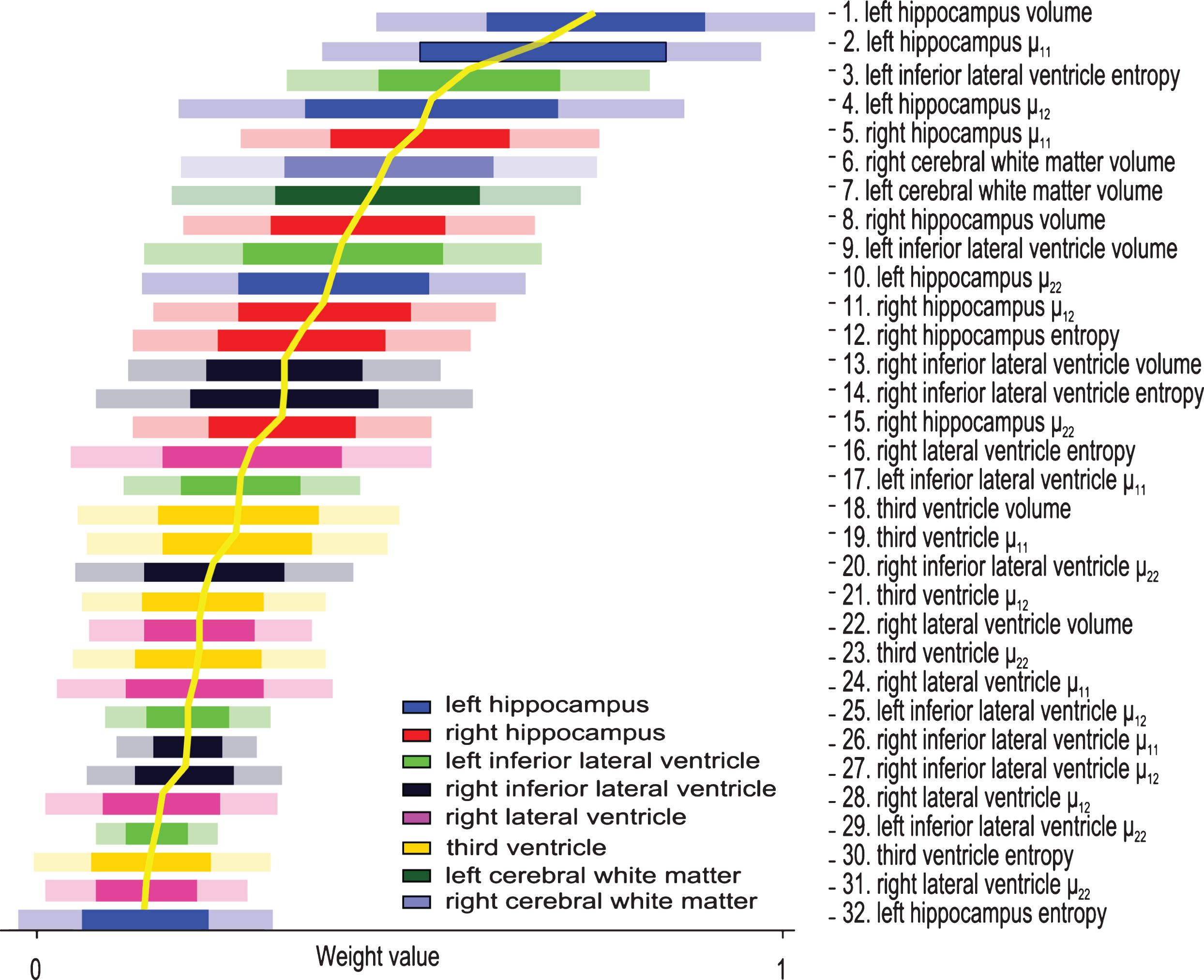
To describe the diagnosticity of different features on various brain structures, we analyze the feature weights learned on the training set. These are automatically determined during the training process and are indicative of the importance of the feature to the classifier [20, 21]. In a sense, our framework automatically prunes the feature space to find the most diagnostic biomarkers, as well as identifies the structures most affected by the disease. Fig. 4 displays the weights of the features ± their standard deviation. To better visualize the importance of the different features, they are sorted in a descending manner, most discriminative on top. All features calculated on the same ROI are displayed in the same color - see Figure legend for quick reference. Left hippocampus automatically emerges as the brain structure most affected by AD since most features calculated on it received high weights. Indeed, MRI derived hippocampal volume strongly correlates with severity of AD pathology as well as memory impairment [22].
DISCUSSION
In the search for robust imaging biomarkers for AD, a range of studies suggest that applying statistical learning techniques on structural MRI data may yield good results in AD classification. A comprehensive review of these studies can be found in [6]. Previous work can be roughly categorized into two groups depending on the types of features extracted from MRI data. Voxel-based techniques use the most basic information of the data - intensity values of the voxels (i.e., the probability of a voxel belonging to one of three tissue types: gray matter, white matter, or cerebrospinal fluid) as the training data for the classifier. Some examples of these works are [23, 24]. Most methods, however, begin with segmentation of the brain into different structures/tissues. Image processing feature extraction techniques are then employed to reduce the dimensionality of the imaging data prior to the classification. These methods differ by the feature extraction methods, the considered ROIs and the classification techniques. In [25] for example, all brain structures are utilized in the classification: voxels are first grouped into regions by registration with a labeled atlas. Intensity histograms of all ROIs are then used as feature vectors, fed into a statistical learning framework.
Recently, most attention has focused on the ROI-based approach which analyzes the volume or shape of a specific brain structure. The hippocampus has received most attention, with classification based on volume or shape-related features. Examples to the latter are [26] and [27], where spherical harmonics (SPHARM) coefficients calculated on the hippocampi are used as a feature vector for the classification. Some recent work has focused on understanding the change in brain ventricles as well [28–30]. These shape-related features are also referred to as shape-descriptors as they describe some attribute of the 3D shape. A comprehensive survey on shape representation can be found in [31]. A comprehensive survey of 3D shape descriptors can be found in [32].
In the context of machine learning, descriptors are referred to as features, and a set of descriptors per shape is referred to as feature vector. The most common and direct way to differentiate between NC, AD, and MCI populations is the volumetric analysis, in which volumes of different brain structures are compared across subjects. These studies differ in the chosen ROIs, the method by which the segmentation of the ROIs is obtained, and the statistical methods used for data analysis. Some examples are [33, 34]. A limitation of the volume-based methods is the inability to capture the more subtle shape changes which happen on a local scale. This limitation is what our work attempts to address.
A recent work [35] has utilized a classical computer vision method [36] and kernel-SVMs for classification of AD subjects and the brain regions most related to the disease. They modified the EigenBrain method first introduced by [37] and proved its effectiveness in AD subject prediction and discriminating affected brain regions on MRI data. In another recent work [38], an average ’displacement field’ is calculated between key-slices in the MRI data between AD subjects and normal controls. These displacement field images are then reduced by principle component analysis and classification is performed by three different SVM variants. This method achieves an impressive classification accuracy on a subset of data from the OASIS dataset (http://www.oasis-brains.org/).
Our work suggests a different approach—our focus is not on the images directly, but rather on the shapes of brain structures affected by AD. The features we derive are shape based and thus capture the subtle changes in tissue degeneration of an ensemble of brain structures.
Identifying MCI subjects that are prone to convert to clinical AD is crucial in developing efficient early prognostic indicators and treatment plans that may delay the onset of cognitive and behavioral symptoms and ultimately improve the quality of life for AD patients and their caregivers. In this paper, we described a fully automatic framework for classification of AD, MCIc, and normal controls. We incorporate shape information from an ensemble of regions of interests in the brain and utilize machine learning approach to build a classifier for each of these populations. The framework is modular, allowing a user-defined choice of ROIs and feature descriptors. In this work we chose to limit the number of structures and focused on the hippocampi and the ventricles. Our framework achieves classification accuracy of 88.13% for NC versus MCIc outperforming other methods. We believe that several factors contribute to this improvement: (1) using an ensemble of ROIs rather than using a single ROI (e.g., hippocampus) or the whole brain data. The ROIs we chose in this study are the structures we believe manifest most shape change in AD; (2) using shape descriptors rather than voxel value data. This allowed us to use a compact descriptor per subject - only 32 numbers. Given the modest amount of data available for training and evaluation, using compact descriptor benefits the classifier learning and avoids overfitting.
The descriptors we used in this work are simple to compute, allow compact representation of the shape, and are effective for classification as they capture the subtle shape changes caused by tissue degeneration. A vast variety of other shape representation exists (see [31] for a comprehensive survey) and may be explored in future work.
In addition to classification, and perhaps more important, is the ability of our framework to automatically identify the structures most affected by the disease. We explored the discriminative power of the different structures and their shape attributes. The hippocampus was automatically found to be the most important structure for the classifier, a notion well supported by the literature. We are encouraged by these results and in future development of this framework we plan to build upon this ability and expand the ROI inputs to identify other potential affected areas. Utilization of this framework in identification of most affected structures in other neurological disorders is also an exciting avenue to explore.
ACKNOWLEDGMENTS
The authors would like to thank Dr. Raif Rustamov and Dr. Adrian Butscher for helpful discussions, Prof. Brian Wandell for providing the computation resources, and Michael Perry for technical support.
T. Glozman is supported by the Stanford Interdisciplinary Graduate Fellowship affiliated with the Stanford Neurosciences Institute; J. Solomon is supported by NSF Mathematical Sciences Postdoctoral Research Fellowship (award number 1502435); F. Pestilli is supported by Indiana University and by Indiana Clinical and Translational Institute (CTSI; NIH UL1TR0011808 A. Shekhar). Data collection and sharing for this project was funded by the Alzheimer’s Disease Neuroimaging Initiative (ADNI) (National Institutes of Health Grant U01 AG024904) and DOD ADNI (Department of Defense award number W81XWH-12-2-0012). ADNI is funded by the National Institute on Aging, the National Institute of Biomedical Imaging and Bioengineering, and through generous contributions from the following: AbbVie, Alzheimer’s Association; Alzheimer’s Drug Discovery Foundation; Araclon Biotech; BioClinica, Inc.; Biogen; Bristol-Myers Squibb Company; CereSpir, Inc.; Cogstate; Eisai Inc.; Elan Pharmaceuticals, Inc.; Eli Lilly and Company; EuroImmun; F. Hoffmann-La Roche Ltd and its affiliated company Genentech, Inc.; Fujirebio; GE Healthcare; IXICO Ltd.; Janssen Alzheimer Immunotherapy Research & Development, LLC.; Johnson & Johnson Pharmaceutical Research & Development LLC.; Lumosity; Lundbeck; Merck & Co., Inc.; Meso Scale Diagnostics, LLC.; NeuroRx Research; Neurotrack Technologies; Novartis Pharmaceuticals Corporation; Pfizer Inc.; Piramal Imaging; Servier; Takeda Pharmaceutical Company; and Transition Therapeutics. The Canadian Institutes of Health Research is providing funds to support ADNI clinical sites in Canada. Private sector contributions are facilitated by the Foundation for the National Institutes of Health (http://www.fnih.org). The grantee organization is the Northern California Institute for Research and Education, and the study is coordinated by the Alzheimer’s Therapeutic Research Institute at the University of Southern California. ADNI data are disseminated by the Laboratory for Neuro Imaging at the University of SouthernCalifornia.
Authors’ disclosures available online (http://j-alz.com/manuscript-disclosures/16-0900r1).
Notes
2 Only the volume of these structures was part of the feature vectors.
REFERENCES
[1] | Brookmeyer R , Johnson E , Ziegler-Graham K , Arrighi HM ((2007) ) Forecasting the global burden of Alzheimer’sdisease. Alzheimers Dement 3: , 186–191. |
[2] | Braak H , Braak E , Bohl J ((1993) ) Staging of Alzheimer-related cortical destruction. Eur Neurol 33: , 403–408. |
[3] | Bruscoli M , Lovestone S ((2004) ) Is MCI really just early dementia? A systematic review of conversion studies. Int Psychogeriatr 16: , 129–140. |
[4] | Fields RD ((2008) ) White matter in learning, cognition and psychiatric disorders. Trends Neurosci 31: , 361–370. |
[5] | Jack CR Jr , Bernstein MA , Fox NC , Thompson P , Alexander G , Harvey D , Borowski B , Britson PJ , L Whitwell J , Ward C , Dale AM , Felmlee JP , Gunter JL , Hill DL , Killiany R , Schuff N , Fox-Bosetti S , Lin C , Studholme C , DeCarli CS , Krueger G , Ward HA , Metzger GJ , Scott KT , Mallozzi R , Blezek D , Levy J , Debbins JP , Fleisher AS , Albert M , Green R , Bartzokis G , Glover G , Mugler J , Weiner MW ((2008) ) The Alzheimer’s Disease Neuroimaging Initiative (ADNI): MRI methods. J Magn Reson Imaging 27: , 685–691. |
[6] | Cuingnet R , Gerardin E , Tessieras J , Auzias G , Lehéricy S , Habert MO , Chupin M , Benali H , Colliot O ((2011) ) Automatic classification of patients with Alzheimer’s disease from structural MRI: A comparison of ten methods using the ADNI database. Neuroimage 56: , 766–781. |
[7] | Dale AM , Fischl B , Sereno MI ((1999) ) Cortical surface-based analysis – segmentation and surface reconstruction. Neuroimage 9: , 179–194. |
[8] | Desikan RS , Ségonne F , Fischl B , Quinn BT , Dickerson BC , Blacker D , Buckner RL , Dale AM , Maguire RP , Hyman BT , Albert MS , Killiany RJ ((2006) ) An automated labeling system for subdividing the human cerebral cortex on MRI scans into gyral based regions of interest. Neuroimage 31: , 968–980. |
[9] | Ferrarini L , Palm WM , Olofsen H , van Buchem MA , Reiber JHC , Admiraal-Behloul F ((2006) ) Shape differences of the brain ventricles in Alzheimer’s disease. Neuroimage 32: , 1060–1069. |
[10] | Wold H ((1966) ) Estimation of principal components and related models by iterative least squares. In Multivariate Analysis, Krishnaiah PR , ed. Academic Press, NY, pp. 391–420. |
[11] | Hu MK ((1962) ) Visual pattern recognition by moment invariants, computer methods in image analysis. IEEE Trans Inf Theory 8: , 179–187. |
[12] | Zhang Y , Yang J , Wang S , Dong Z , Phillips P ((2016) ) Pathological brain detection in MRI scanning via Hu moment invariants and machine learning. J Exp Theor Artif Intell. 1–14. doi: 10.1080/0952813X.2015.1132274 |
[13] | Wang S , Lu S , Dong Z , Yang Z , Yang M , Zhang Y ((2016) ) Dual-tree complex wavelet transform and twin support vector machine for pathological brain detection. Appl Sci 6: , 169. |
[14] | Wang S , Yang X , Zhang Y , Phillips P , Yang J , Yuan TF ((2015) ) Identification of green, oolong and black teas in china via wavelet packet entropy and fuzzy support vector machine. Entropy 17: , 6663–6682. |
[15] | Cortes C , Vapnik V ((1995) ) Support-vector networks. Mach Learn 20: , 273–297. |
[16] | Fan RE , Chang KW , Hsieh CJ , Wang XR , Lin CJ ((2008) ) LIBLINEAR: A library for large linear classification. J Mach Learn Res 9: , 1871–1874. |
[17] | Lalkhen AC , McCluskey A ((2008) ) Clinical tests: Sensitivity and specificity. Contin Educ Anaesth Crit Care Pain 8: , 221–223. |
[18] | Macmillan NA , Creelman CD ((2004) ) Detection theory: A user’s guide. Lawrence Erlbaum Associates, Inc. |
[19] | Heeger D ((1997) ) Signal detection theory, teaching handout.. Department of Psychology, Stanford University, Stanford, CA USA. |
[20] | Guyon I , Weston J , Barnhill S , Vapnik V ((2002) ) Gene selection for cancer classification using support vector machines. Mach Learn 46: , 389–422. |
[21] | Chang YW , Lin CJ ((2008) ) Feature ranking using linear SVM. J Mach Learn Res 3: , 53–64. |
[22] | Jack CR Jr , Dickson DW , Parisi JE , Xu YC , Cha RH , O’Brien PC , Edland SD , Smith GE , Boeve BF , Tangalos EG , Kokmen E , Petersen RC ((2002) ) Antemortem MRI findings correlate with hippocampal neuropathology in typical aging and dementia. Neurology 58: , 750–757. |
[23] | Querbes O , Florent A , Pariente J , Lotterie JA , Demonet JF , Duret V , Puel M , Berry I , Fort JC , Celsis P ((2009) ) Early diagnosis of Alzheimer’s disease using cortical thickness: impact of cognitive reserve. Brain 132: , 2036–2047. |
[24] | Casanova R , Hsu FC , Sink KM , Rapp SR , Williamson JD , Resnick SM , Espeland SM ((2013) ) Alzheimer’s disease risk assessment using large-scale machine learning methods. PLoS One 8: , e77949. |
[25] | Magnin B , Mesrob L , Kinkingnéhun S , Pélégrini-Issac M , Colliot O , Sarazin M , Dubois B , Lehéricy S , Benali H ((2009) ) Support vector machine-based classification of Alzheimer’s disease from whole-brain anatomical MRI. Neuroradiology 51: , 73–83. |
[26] | Colliot O , Chételat G , Chupin M , Desgranges B , Magnin B , Benali H , Dubois B , Garnero L , Eustache F , Lehéricy S ((2008) ) Discrimination between Alzheimer disease, mild cognitive impairment, and normal aging by using automated segmentation of the hippocampus. Radiology 248: , 194–120. |
[27] | Gerardin E , Chételat G , Chupin M , Cuingnet R , Desgranges B , Kim HS , Niethammer M , Dubois B , Lehéricy S , Garnero L , Eustache F , Colliot O ((2009) ) Multidimensional classification of hippocampal shape features discriminates Alzheimer’s disease and mild cognitive impairment from normal aging. Neuroimage 47: , 1476–1486. |
[28] | Ferrarini L , Palm WM , Olofsen H , van Buchem MA , Reiber JH , Admiraal-Behloul F ((2006) ) Shape differences of the brain ventricles in Alzheimer’s disease. Neuroimage 32: , 1060–1069. |
[29] | Nestor SM , Rupsingh R , Borrie M , Smith M , Accomazzi V , Wells JL , Fogarty J , Bartha R ((2008) ) Ventricular enlargement as a possible measure of Alzheimer’s disease progression validated using the Alzheimer’s disease neuroimaging initiative database. Brain 131: , 2443–2454. |
[30] | Shi J , Stonnington CM , Thompson PM , Chen K , Gutman B , Reschke C , Baxter LC , Reiman EM , Caselli RJ , Wang Y ((2015) ) Studying ventricular abnormalities in mild cognitive impairment with hyperbolic ricci flow and tensor-based morphometry. Neuroimage 104: , 1–20. |
[31] | Zhang D , Lu G ((2004) ) Review of shape representation and description techniques. Pattern Recognition 37: , 1–19. |
[32] | Tangelder JW , Veltkamp RC ((2008) ) A survey of content based 3d shape retrieval methods. Multimedia Tools Applications 39: , 441–471. |
[33] | Jiji S , Smitha KA , Gupta AK , Pillai VPM , Jayasree RS ((2013) ) Segmentation and volumetric analysis of the caudate nucleus in Alzheimer’s disease. Eur J Radiol 82: , 1525–1530. |
[34] | Gosche KM , Mortimer JA , Smith CD , Markesbery WR , Snowdon DA ((2002) ) Hippocampal volume as an index of Alzheimer neuropathology. Neurology 58: , 1476–1482. |
[35] | Zhang Y , Wang S , Phillips P , Jiquan Y , Ti-Fei Y ((2016) ) Three-dimensional eigenbrain for the detection of subjects and brain regions related with Alzheimer’s disease. J Alzheimers Dis 50: , 1163–1179. |
[36] | Turk MA , Pentland AP ((1991) ) Face recognition using eigenfaces., pp. IEEE conference on Computer vision and Pattern Recognition 586–591. |
[37] | Alvarez I , Gorriz JM , Ramirez J , Salas-Gonzalez D , Lopez M , Puntonet CG , Segovia F ((2009) ) Alzheimers diagnosis using eigenbrains and support vector machines. Bio-Inspired Syst Comput Ambient Intell 5517: , 973–980. |
[38] | Wang S , Zhang Y , Ge L , Phillips P , Ti-Fei Y ((2016) ) Detection of Alzheimer’s disease by three-dimensional displacement field estimation in structural magnetic resonance imaging. J Alzheimers Dis 50: , 233–248. |
Figures and Tables
Fig.1
Overall tissue loss in the brain in AD patient (right) versus normal control (left) in coronal and axial views. The labeled regions are: (a) lateral ventricles; (b) hippocampi; and (c) cerebral cortex.
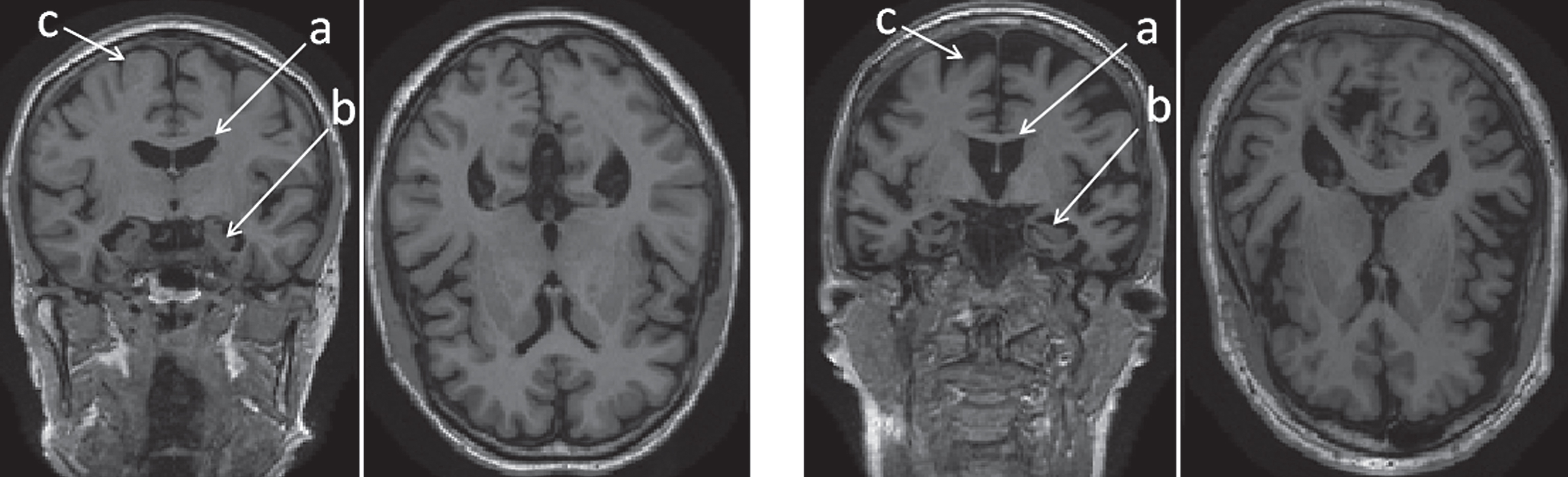
Fig.2
Change in shape of brain structures in AD manifested on projection images. (a) l. hippocampus 3D shape (upper panel) in NC (left) and AD (right). (b) l. inf. lat. ventricle 3D shape (upper panel) in healthy control (left) and AD patient (right). Lower panel shows the corresponding canonical view using our principal projections method.
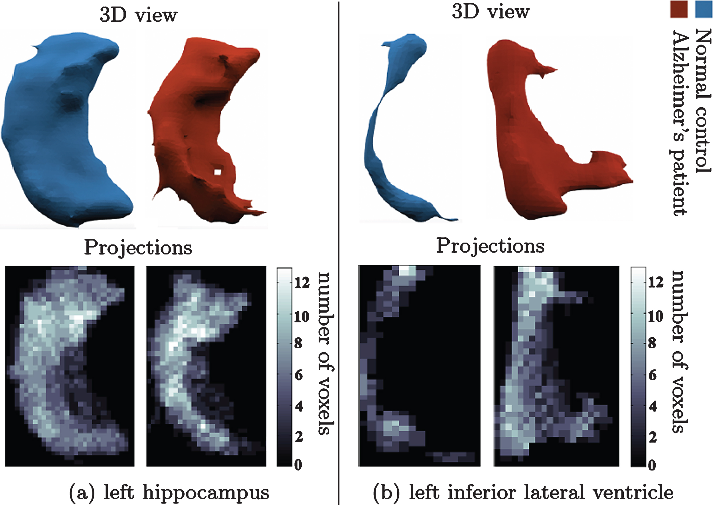
Fig.3
Comparison to other methods. D’, sensitivity, and specificity for NC versus AD and NC versus MCIc classification. Our method (red dot) outperforms previous methods in NC versus MCIc classification, indicating applicability for identifying patients with higher risk of conversion to AD.
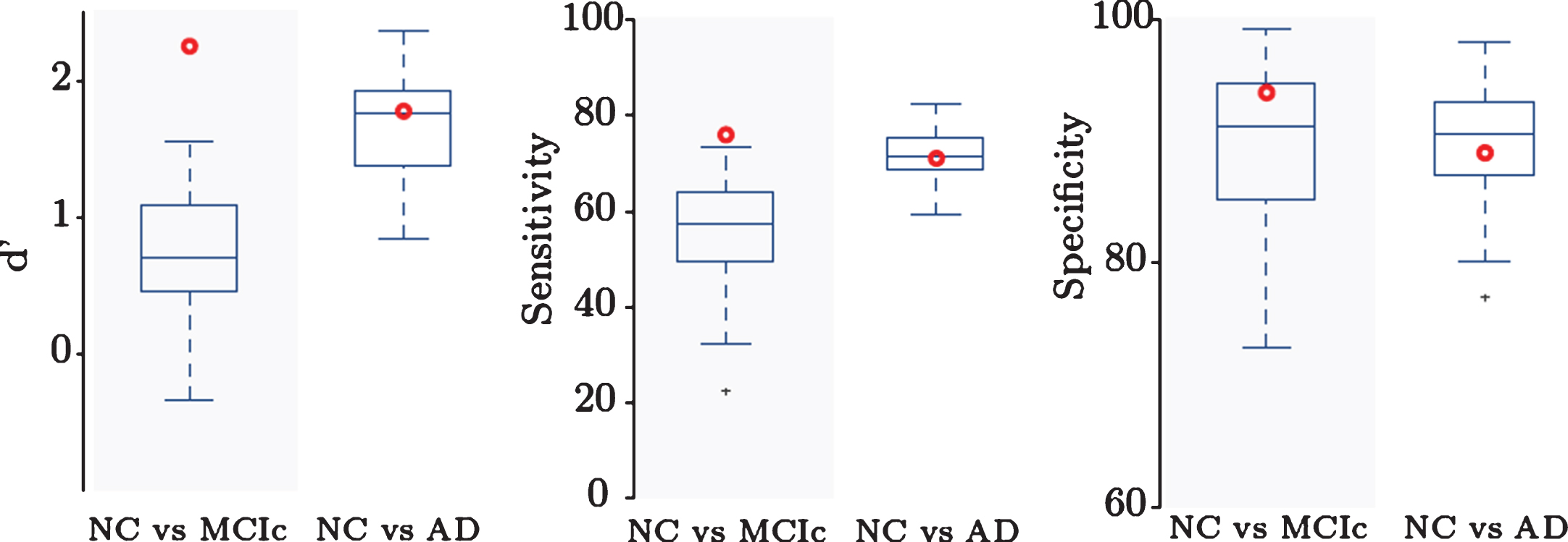
Fig.4
Diagnosticity for different shape attributes of various ROIs. Features sorted and numbered according to their respective descending weights in AD versus NC classification. Feature number represents relative rank-order. Weights values suggest the relative significance of the feature to the classifier, i.e., the diagnostic power of the feature. Colors correspond to different brain structures as outlined in the legend.