An efficient approach to directly compute the exact Hausdorff distance for 3D point sets

Zhang, Dejun; He, Fazhi; Han, Soonhung; Zou, Lu; Wu, Yiqi; Chen, Yilin

doi:10.3233/ICA-170544

An efficient approach to directly compute the exact Hausdorff distance for 3D point sets

Article type: Research Article

Authors: Zhang, Dejun^{a; b} | He, Fazhi^{a; d; *} | Han, Soonhung^c | Zou, Lu^b | Wu, Yiqi^a | Chen, Yilin^a

Affiliations: [a] School of Computer Science, Wuhan University, Wuhan, Hubei, China | [b] College of Information and Engineering, Sichuan Agricultural University, Yaan, Sichuan, China | [c] Division of Ocean Engineering, Korea Advanced Institute of Science and Technology, Daejeon, Korea | [d] State Key Laboratory of Digital Manufacturing Equipment and Technology, Huazhong University of Science and Technology, Wuhan, Hubei, China

Correspondence: [*] Corresponding author: Fazhi He, School of Computer Science, Wuhan University, Wuhan, Hubei, China. E-mail: [email protected].

Keywords: Hausdorff distance, 3D point sets, similarity, octree, branch and bound, runtime analysis

DOI: 10.3233/ICA-170544

Journal: Integrated Computer-Aided Engineering, vol. 24, no. 3, pp. 261-277, 2017

Published: 21 July 2017

Get PDF

Abstract

Hausdorff distance measure is very important in CAD/CAE/CAM related applications. This manuscript presents an efficient framework and two complementary subalgorithms to directly compute the exact Hausdorff distance for general 3D point sets. The first algorithm of Nonoverlap Hausdorff Distance (NOHD) combines branch-and-bound with early breaking to cut down the Octree traversal time in case of spatial nonoverlap. The second algorithm of Overlap Hausdorff Distance (OHD) integrates a point culling strategy and nearest neighbor search to reduce the number of points traversed in case of spatial overlap. The two complementary subalgorithms can achieve a highly efficient and balanced result. Both NOHD and OHD compute the exact Hausdorff distance directly for arbitrary 3D point sets. We conduct a number of experiments on benchmark models and CAD application models, and compare the proposed approach with other state-of-the-art algorithms. The results demonstrate the effectiveness of our method.

1.Introduction

Distance measure is the fundamental step for many applications in science and engineering areas [15, 41, 68]. Hausdorff distance can quantify the similarity between two arbitrary point sets without the necessity to establish the one-to-one correspondence between them. In most engineering applications, the number of point sets obtained by 3D model is not identical, and it is difficult to establish a one-to-one correspondence between them. Therefore, Hausdorff distance is suitable for measuring similarity between 3D models in engineering practice.

Hausdorff distance has drawn particular attention from scholars in many science and engineering fields, such as CAE/CAD/CAM [40, 68], pattern recognition [52, 63], similarity measure [16, 30, 32, 48], shape matching [5, 70], mesh model simplification [26], reconstruction of curved and surfaces [11, 12, 18, 35], and penetration depth [66, 73].

It is a hard task to improve the efficiency of the algorithm while ensuring the accuracy in calculating the Hausdorff distance. Generally speaking, the similarity measure for 3D models based on Hausdorff distance faces at least three problems: (1) Most of the previous algorithms of similarity measure based on Hausdorff distance have a strong disciplinary background, and are short of generalization; (2) Since the Hausdorff distance measure is computationally intensive, it is restricted to applications for large scale data; (3) Furthermore, in some applications, computing exact Hausdorff distance needs additional cost (for example, 3D point sets are pre-processed and rasterized into voxel models), which worsen efficiency of some state-of-the-art algorithms.

To the best of our knowledge, it is difficult to cover above limitations in one single processing algorithm. For an example, the state-of-the-art algorithm of 2015 (EARLYBREAK) [65] can achieve the high efficiency in processing the medical images (considered as voxel data), while it is low efficiency in calculating spatial objects of highly overlapping.

How to find a new approach to cover above problems as much as possible and achieve an efficient and balanced result is becoming a challenge. In this manuscript, based on whether the pair of point sets are nonoverlaped or overlaped, an efficient computation framework is presented with two complementary subalgorithms, Nonoverlap Hausdorff Distance (NOHD) and Overlapped Hausdorff Distance (OHD).

• The NOHD algorithm builds an Octree for input point sets, and uses the principle of branch-and-bound and early breaking to prune the branches of Octree efficiently, which can reduce the number of nodes that have to be traversed.
• However, the efficiency is poor when applying the NOHD algorithm to two point sets of seriously overlapped. Therefore, we propose the OHD algorithm to solve this problem. The OHD algorithm builds adaptive Octree, and also designs point culling strategy which can reduce the traversed points. Both NOHD and OHD compute the exact Hausdorff distance directly for arbitrary 3D point sets. Under the subalgorithms of NOHD and OHD, we present a new Hausdorff distance computing procedure, which can choose the complementary subalgorithms to compute the Hausdorff distance with different spatial relationship of the pair of point sets.

The remainder of this manuscript is organized as follows. In Section 2, we briefly review the related work. Section 3 describes the problem and challenge for computing Hausdorff distance. In Section 4, we present two novel subalgorithms, the NOHD algorithm and the OHD algorithm. In Section 5 we construct an integrated framework of computing the Hausdorff distance. Section 6 conducts experiments with analysis. Finally, the conclusions and future work are discussed in Section 7.

2.Related work

The research of Hausdorff distance originated from computer vision [23, 25, 31, 46, 59, 61, 62] and was quickly extended to many areas of science and engineering [5, 9, 13, 40, 41, 68].

2.1Curves and surfaces

The problem of efficient calculation of the Hausdorff distance has become a hot topic in this field, has influenced the progress in CAD/CAE/CAM.

Alt et al. [7] presented an algorithm for Hausdorff distance computation based on a characterization of the possible points where the distance can be attained. Chen et al. [18] presented an algorithm for computing the Hausdorff distance between two B-Spline curves, which improves the reference [7] by using a pruning technique to reduce computation time.

Bai et al. [11] presented an algorithm for computing an approximate Hausdorff distance between planar free-form curves by approximating the input curves with polylines and then computing the Hausdorff distance between the line segments. Kim et al. [34] presented a compact representation for the Bounding Volume Hierarchy (BVH) of Non-uniform rational Basis spline (NURBS) surfaces using Coons patches, which could be used to construct a BVH-based algorithm for computing the Hausdorff distance between NURBS surfaces.

Kim et al. [36] developed a real-time algorithm for the precise Hausdorff distance between planar freeform curves using hardware depth buffer.

Recently, Krishnamurthy et al. [28, 38, 39] developed a GPU algorithm that computes the Hausdorff distance between NURBS surfaces. Interactive speeds are obtained by performing GPU traversal of a bounding-box hierarchy and selectively culling pairs of bounding boxes that could not contribute to the Hausdorff distance.

2.2Polygonal models

The Hausdorff distance computation for large polygonal meshes has been a very difficult task to implement for real-time application.

Atallah [9] provided an algorithm for computing the Hausdorff distance for a special case of point sets, namely non-intersecting, convex polygons. The algorithm has the complexity of O⁢(n+m) where m and n are the vertex counts. Alt et al. [5] presented a method based on the Voronoi diagram which requires O⁢((n+m)⁢log⁡(n+m)) running time. Barton et al. [39] presented an O⁢(n4⁢log⁡n) deterministic algorithm for computing the precise (up to floating point) Hausdorff distance between polygonal meshes.

Due to the complexity of exactly computing the Hausdorff distance, the approximate algorithms have been proposed as practically solutions [8, 22, 26, 47]. Llanas [47] proposed two approximate algorithms based on random covering for non-convex polytopes. Guthe et al. [26] proposed an approximate algorithm for calculating the Hausdorff distance between mesh surfaces. This algorithm makes use of the specific characteristics of meshes to avoid sampling all points in the compared surfaces. These regions are then further subdivided and regions that cannot attain the Hausdorff distance are purged away.

Tang et al. [66] implemented an approximate algorithm that is based on BVH that is preprocessed in advance (before real-time computation). Their implementation is very fast in practice, running at interactive speed for complicated dynamics scene.

2.3Point sets

Above algorithms are based on the specific characteristics of meshes and thereby lacks generality. Some general methods are proposed. Given two nonempty point-sets with n and m points respectively, a brute-force algorithm to compute the Hausdorff distance requires O⁢(n×m) time.

Alt et al. [5] presented a method based on the Voronoi diagram which requires O⁢((n+m)⁢log⁡(n+m)) running time. For R3, Alt et al. [6] proposed a randomized algorithm with O((n+m+(nm)3/4)log(n+m)) expected time. Papadias et al. [55] proposed an algorithm for finding aggregate nearest neighbors (ANN) in databases.

Nutanong et al. [54] extended the algorithm proposed in [55] to avoid the iteration of all points in A. The aggregate nearest neighbor was executed simultaneously in both directions, where two R-Trees (one for each point set) were used at the same time.

Taha et al. proposed the randomization and the early breaking optimization in reference [65] to achieve efficient, almost linear, calculation. This optimization avoid scanning all voxel pairs by identifying and skipping unnecessary rounds.

The purpose of this study is to explore a general method to compute the exact Hausdorff distance for CAD/CAE/CAM applications and to ensure the efficiency.

3.Problem state

3.1Hausdorff distance

The Hausdorff distance [66] is the maximum deviation between two models, measuring how far two point sets are from each other [26]. Given two nonempty point sets A={x1,x2,…,xn} and B={y1,y2,…,ym}, the Hausdorff distance between A and B is defined as H⁢(A,B).

(1)

H⁢(A,B)=max⁡(h⁢(A,B),h⁢(B,A))

where

(2)

h⁢(A,B)=maxx∈A⁡(miny∈B⁡∥x-y∥)

(3)

h⁢(B,A)=maxy∈B⁡(minx∈A⁡∥y-x∥)

H⁢(A,B) denotes the Hausdorff distance in R3. h(B,A) and h(A,B) are the one-sided value from A to B and from B to A, respectively.

The Hausdorff distance is often used in engineering and science for pattern recognition, shape matching and error controlling. If H⁢(A,B) is a small value, A and B are partially matched; If H⁢(A,B) is equal to zero, then A and B are matched exactly.

3.2NAIVEHDD and one-side BREAK algorithm

The basic computing method of the Hausdorff distance is described as Algorithm 1.

The outer loop of the NAIVEHDD algorithm traverses all points in A, while the inner loop traverses all points in B. The time complexity of NAIVEHDD algorithm is O⁢(m×n).

Algorithm 1. NAIVENDD algorithm

Input: Two finite point sets A, BOutput: Directed Hausdorff distance

1. cmax← 0
2. forx∈Ado
3. cmax←∞
4. fory∈Bdo
5. d←∥x,y∥
6. 𝑐𝑚𝑖𝑛←𝑚𝑖𝑛⁢{cmin, d}
7. end for
8. 𝑐𝑚𝑎𝑥←𝑚𝑎𝑥⁢{cmax, cmin}
9. end for
10. returncmax

Taha et al. [65] pointed out that it is not necessary for inner loop (4 ∼ 7 lines) of the NAIVEHDD algorithm to traverse all points in B, and proposed an early break strategy in Algorithm 2. In the inner loop of Algorithm 2, when a distance is found that is below the current cmax, continuing to traverse the remaining points in B makes no contribution to update cmax. Therefore, the breaking of the inner loop at that time will reduce the cost of traversing B. In the best case when the inner loop meets the breaking condition at the first execution and then break, the ideal time complexity of the EARLYBREAK algorithm is O⁢(m).

The original algorithm published in [65] missed one line and had been corrected in a note.

Algorithm 2. EARLYBREAK algorithm

Input: Two finite point sets A, BOutput: Directed Hausdorff distance

1. cmax← 0
2. Ar← randomize(A)
3. Br← randomize(B)
4. forx∈Ardo
5. cmin←∞
6. fory∈Brdo
7. d←∥x, y∥
8. Ifd < cmaxthen
9. cmin← 0
10. break
11. end if
12. 𝑐𝑚𝑖𝑛←𝑚𝑖𝑛⁢{cmin, d}
13. end for
14. 𝑐𝑚𝑎𝑥←𝑚𝑎𝑥⁢{cmax, cmin}
15. end for
16. returncmax

3.3Challenge and analysis

In Algorithm 2, the event of meeting the condition that d is over cmax is denoted as e, P⁢(e)=q. The event of meeting the condition that d is less than cmax is denoted as e, P⁢(𝑒¯)=p=1-q. the breaking condition for the inner loop (6 ∼12 lines) is that event e occurs.

Assuming that the inner loop has been implemented for R times before the loop terminates, then the probability density function of R can be expressed as:

f(x)=P(d1>𝑐𝑚𝑎𝑥,…,dx-1>𝑐𝑚𝑎𝑥,

dx⩽𝑐𝑚𝑎𝑥)

(4)

=qx-1⁢p

The expectation of R (the number of execution of the inner loop) is equal to the expectation of f⁢(x),

(5)

E⁢(R)=∑x=1∞x⁢f⁢(x)=∑x=1∞x⁢qx-1⁢p=1p

According to Eq. (5), the number of tries in the inner loop is inverse proportion to q. Meanwhile, Taha et al. [65] pointed out that p depends on h⁢(A,B) and the distribution of all the pair of distances between A and B, rather than directly on the number of B.

The larger h⁢(A,B) is, the larger cmax is, and the larger p is. The average probability of the breaking condition can be expressed as:

(6)

p¯=𝑎𝑣𝑒𝑟𝑎𝑔𝑒⁢(∫x=0𝑐𝑚𝑎𝑥g⁢(x)⁢𝑑x)=c⁢∫x=0Hg⁢(x)⁢𝑑x

Where g⁢(x) represents the probability distribution function of all the distances between A and B, and c is a constant representing the relationship between cmax and the final Hausdorff distance.

After substituting Eq. (6) into Eq. (5), the expectation of R can be obtained as:

(7)

E⁢(R)=1P¯=1c⁢∫x=0hg⁢(x)⁢𝑑x

It should be noticed that the smaller h⁢(A,B) is, the larger R is, leading to a decreased efficiency of the EARLYBREAK algorithm. In the worst case, when the h⁢(A,B) between A and B is equal to zero, the inner loop will traverse all the points in B, and the time complexity of the EARLYBREAK algorithm is equal to that of NAIVEHDD algorithm.

In order to overcome the deficiency in overlap situation, Taha and Hanbury [65] proposed a strategy to exclude the intersection point set between A and B. As shown in Fig. 1, for given grid sets AG (brown box in Fig. 1(a)) and BG (blue box in Fig. 1(b)), {AG}∩{BG} (green box in Fig. 1(c)) is first calculated. Then the grid set EG is computed as EG={AG}-{AG}∩{BG}. At last, the EG is used to calculate the Hausdorff distance in EARLYBREAK algorithm as h⁢(EG,BG).

Figure 1.

Excluding intersection in EARLYBREAK. (a) AG; (b) BG; (c) {AG}∩{BG}; (d) EG.

According to the property of Hausdorff distance, h⁢(AG,BG)=h⁢(EG,BG). Obviously, the time complexity of h⁢(EG,BG) is significantly better than that of h⁢(AG,BG). Therefore, the EARLYBREAK algorithm has achieved outstanding results in calculating the Hausdorff distance of medical images.

There are still some problems for EARLYBREAK algorithm [65]. Firstly, the execution number of the inner loop was reduced by early breaking and random initialization, but the execution number of the outer loop was not reduced. Secondly, when the similarity between A and B is high (e.g., the Hausdorff distance is small), the strategy of early breaking fails to reduce the time complexity. Thirdly, the EARLYBREAK algorithm is inherently and naturally suitable for voxel model and medical image, not for general 3D model, such as 3D point cloud in CAD/CAE/CAM. Finally, if we simply apply the EARLYBREAK algorithm for general 3D models, the original 3D model have to be preprocessed and rasterized into voxel model, which is the approximation for the original 3D models. Therefore, the final result will be approximate one, not exact one.

This manuscript tries to address the above problems as much as possible, and present a new approach to directly and efficiently calculate the Hausdorff distance for general 3D model with an exact result.

4.The proposed two subalgorithms

Firstly, due to the fact that the two subalgorithms are based on Octree, a set of definitions related to lower bound and upper bound are provided. In the case of spatial nonoverlap, a subalgorithm named NOHD was proposed. Then, we analyzed the complexity for computing the Hausdorff distance in the case of spatial overlap and proposed the OHD algorithm.

4.1The definition of bound and the description of overlap

The Hausdorff distance between A and B can be actually obtained by calculating the Hausdorff distance between A and OctreeB (constructed from B). The principles of branch-and-bound [24] have be adopted in our NOHD and the OHD algorithms to reduce the number of nodes to be traversed. Therefore, before presenting the NOHD and OHD algorithms, the related definitions are given as follows.

Definition 1. Lower bound of point to node. Given a singleton set {p} and a node C in an Octree, a lower bound of the Hausdorff distance from p to the elements confined by C is defined as Eq. (8),

(8)

l⁢b⁢(p,C)=min⁡{𝐷𝐼𝑆𝑇⁢(p,𝑜𝑏𝑗𝑒𝑐𝑡):𝑜𝑏𝑗𝑒𝑐𝑡∈C}

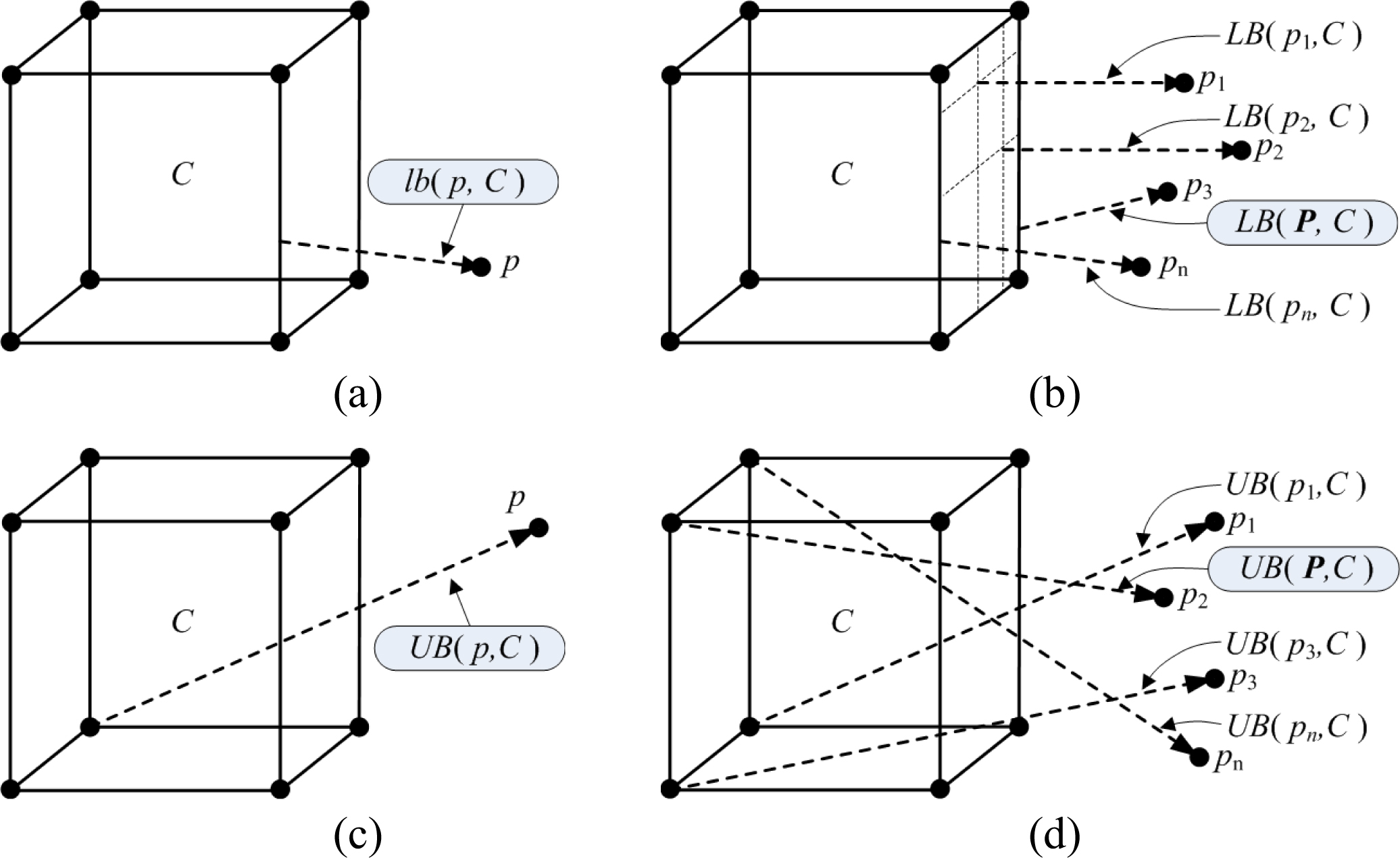
As shown in Fig. 2(a), the lb(p,C) of Hausdorff distance between point p and node C can be obtained by calculating the minimum possible distance between point p and the nearest object (vertexes, edges, surfaces) of node C.

Definition 2. Lower bound of point set to node. Given a point set P and a node C in an Octree, a lower bound of the Hausdorff distance from P to the elements confined by C is defined as Eq. (9),

(9)

𝐿𝐵⁢(P,C)=min⁡{l⁢b⁢(p,C):p∈P}

As shown in Fig. 2(b), the LB(P,C) of Hausdorff distance between the point set P to node C can be obtained by calculating the minimum value of the lower bound between all points in the point set P and node C.

Figure 2.

Lower bound and upper bound of Hausdorff distance: (a) lower bound from point to node; (b) lower bound from points to node; (c) upper bound from point to node; (d) upper bound from points to node.

Definition 3. Upper bound of point to node. Given a singleton set {p} and a node C in an Octree, a upper bound of the Hausdorff distance from p to the elements confined by C is defined as Eq. (10),

(10)

u⁢b⁢(p,C)=max⁡{𝐷𝐼𝑆𝑇⁢(p,𝑣𝑒𝑟𝑡𝑒𝑥):𝑣𝑒𝑟𝑡𝑒𝑥∈C}

As shown in Fig. 2(c), the ub(p,C) of the Hausdorff distance between point p and node C can be obtained by calculating the maximum possible distance between point p and the farthest object (vertex) in node C.

Definition 4. Upper bound of point set to node. Given a point set P and a node C in an Octree, a upper bound of the Hausdorff distance from P to the elements confined by C is defined as Eq. (11),

(11)

𝑈𝐵⁢(P,C)=min⁡{u⁢b⁢(p,C):p∈P}

As shown in Fig. 2(d), the 𝑈𝐵⁢(P,C) of Hausdorff distance from the point set P to node C can be obtained by calculating the minimum value of the upper bound from all points in the point set P to node C.

According to the analysis in Section 3, when the value of Hausdorff distance between A and B is relatively small as two objects overlap, the previous algorithms (including state-of-the-art EARLYBREAK in the reference [65]) cannot efficiently reduce the time complexity. However, the small value of Hausdorff distance occurs in many engineering applications. Therefore, before presenting our algorithms, the overlap is described.

Given an object A in 3D space, the range for bounding box BBA is described as follows:

x∈[xAL,xAU],y∈[yAL,yAU],z∈[zAL,zAU].

Similarly, given an object B in 3D space, the range for bounding box BBB is described as follows:

x∈[xBL,xBU],y∈[yBL,yBU],z∈[zBL,zBU].

In context of this manuscript, the description of overlapping between BBA and BBB can be written as follows.

(12)

Ix={x|xAL⩽x⩽xAU&&xBL⩽x⩽xBU,x∈ℝ}

(13)

Iy={y|yAL⩽y⩽yAU&&yBL⩽y⩽yBU,y∈ℝ}

(14)

Iz={z|zAL⩽z⩽zAU&&zBL⩽z⩽zBU,z∈ℝ}

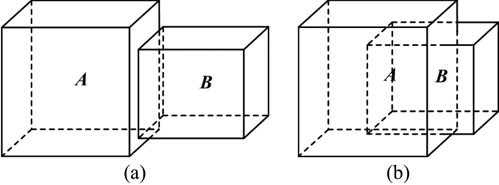
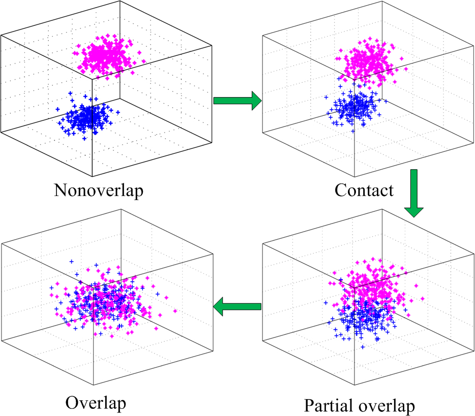
As shown in Fig. 3(a), when Ix=Φ∥Iy=Φ∥Iz=Φ, it is denoted as A∩B=Φ. It means there is nonoverlapping relationship between A and B.

As shown in Fig. 3(b), when Ix≠Φ && Iy≠Φ && Iz≠Φ, it is denoted as A∩B≠Φ. It means there is overlapping relationship between A and B.

Figure 3.

The spatial relations between A and B: (a) nonoverlapping; (b) overlapping.

4.2The first subalgorithm: NOHD

4.2.1The basic idea of NOHD and the definition of priority queue

In order to reduce the outer loop number of traversal of A, the NOHD algorithm is proposed.

Firstly, the calculation of Hausdorff distance from A to B is converted into calculating the Hausdorff distance from OctreeA (constructed from A) to B. The lower bound of the Hausdorff distance from any node N in OctreeA to B is denoted as LB(B,N), and the upper bound of the Hausdorff distance is denoted as UB(B,N). By traversing all the nodes in OctreeA and updating LB(B,N), the final LB(B,N) is the Hausdorff distance between A and B at end of NOHD algorithm.

Secondly, NOHD algorithm defines a new concept of entry of Decreasing Priority Queue (DPQ) to enhanced the principles of branch-and-bound, and therefore to reduce the number of nodes of OctreeA to be traversed. In the context of Hausdorff distance calculation, the definition for entry of DPQ is given as follows.

Definition 5. 𝐸𝑛𝑡𝑟𝑦⁢(𝑁,𝑀𝑖𝑛𝑈𝐵). Attributes of each Entry(N, MinUB) are described as follows: (i) Node N← node in an Octree for A, which could be an object node or a non-object node (index node); (ii) Distance MinUB← the minimum value of the upper bound between all points in the point set B to node N, that is, the UB(B,N).

The DPQ which arranges Entries(N, MinUB) in decreasing order according to the key value of MinUB.

4.2.2NOHD algorithm description

Algorithm 3. NOHD algorithm

Input: Two finite point sets A, BOutput: Directed Hausdorff distance

1. Octree←A Create an Octree for A
2. DPQ← Create a “descending order”
priority queue
3. Insert(((RootOf(OctreeA), ∞), DPQ)
4. MaxLB← 0
5. while (DPQ is not empty) do
6. Entry(N, MinUB) ← Dequeue(DPQ)
7. ifN is a non-object then
8. ifMinUB⩾MaxLBthen
9. for each child node C of Ndo
10. [𝑈𝐵⁢(B,C),𝐿𝐵⁢(B,C),𝐹𝑙𝑎𝑔]←
CubeToPoints (C, B, MaxLB)
11. ifFlag==truethen
12. 𝑀𝑎𝑥𝐿𝐵←max{𝑀𝑎𝑥𝐿𝐵,
𝐿𝐵(B,C)}
13. Insert((C, UB(B,C)), DPQ)
14. end if
15. end for
16. end if
17. Sort DPQ in descending order using
the second element
18. else
19. for each point x of Ndo
20. d← PointToPoints(x; B; MaxLB)
21. 𝑀𝑎𝑥𝐿𝐵←max⁡{MaxLB, d}
22. end for
23. end if
24. end while
25. return MaxLB

The NOHD algorithm is described in Algorithm 3. The initialization involves the following steps: (i) To create an Octree OctreeA for point set A; (ii) To create a priority queue DPQ; (iii) to insert the root of OctreeA with an initial MinUB of ∞ into DPQ. (iv) To initialize MaxLB to 0.

After the initialization, DPQ contains a single entry with the root of OctreeA as the associated node. For each iteration of the while loop (5 ∼ 24 lines), the head Entry(N, MinUB) is removed from DPQ. There are two cases depending on whether N is an object or not.

• In case 1, if N is not a point object, the children of N (8 ∼17 lines) are processed.
• In case 2, if N is a point object (19 ∼22 lines), the minimum distance from point x to point set B is obtained by calling Algorithm 5, and is compared with MaxLB. After comparison, the greater one is the final Hausdorff distance.

In processing of node N, two culling procedures are performed.

The first culling is based on whether MinUB is greater than MaxLB or not, the following steps are processed respectively:

• If MinUB⩾MaxLB, all child nodes in node N should be traversed (9 ∼15 lines);
• If MinUB<MaxLB, node N cannot generate a distance greater than the current MaxLB, and it is pruned away.

In the second culling, CubeToPoints (Algorithm 4) is called, and a breaking flag of child node C is returned.

• If the flag is “false”, the child node C cannot generate a distance that contributes to the final Hausdorff distance, and it is pruned away.
• If the flag is “true”, the child node C may generate a distance that contributes to the final Hausdorff distance, and then it is inserted into DPQ.

The pseudocode of CubeToPoints is described as Algorithm 4, into which three parameters are input: child nodes C, points set B, and the currently greatest lower bound MaxLB.

The Algorithm 4, firstly initializes the flag, the UB(B, C) and LB(B,C), and then computes the upper and lower bounds between all points in B and child node C. For a given point y of B, the upper bound of y to child node C is calculated. If the ub(y, C) is below MaxLB, then the minimum upper bound from all points in B to child node C must be below MaxLB. Thus, child node C cannot generate a distance over MaxLB, and then the Flag is assigned as “false”, and the whole for loop breaks. When the flag of Algorithm 4 is returned as “false”, the node will be pruned away by Algorithm 3.

Algorithm 4. CubeToPoints(C, B, Max LB)

Input: Child Node C, Point set B, MaxLBOutput:UB(B;C), LB(B;C), Flag

1. Flag←true
2. 𝑈𝐵⁢(B,C)←∞,𝐿𝐵⁢(B,C)←∞
3. for each point y of Bdo
4. [𝑢𝑏⁢(y,C),𝑙𝑏⁢(y,C)]←
PointToCube(y,C)
5. if𝑢𝑏⁢(y,C)⩽𝑀𝑎𝑥𝐿𝐵then
6. Flag←false
7. break
8. end if
9. 𝑈𝐵⁢(B;C)←min⁡{𝑈𝐵⁢(B,C),𝑢𝑏⁢(y,C)}
10. 𝐿𝐵⁢(B;C)←min⁡{𝐿𝐵⁢(B,C),𝑙𝑏⁢(y,C)}
11. end for
12. returnUB(B,C), LB(B,C), Flag

The pseudocode of PointToPoints is shown as Algorithm 5, which takes three parameters: point x of node C, points set B, and the greatest lower bound MaxLB.

Algorithm 5 calculates the minimum distance from point x to B. For a given y of B, the distance d of y to x of child node C is calculated. And if d is less than MaxLB, the minimum distance between point x and B must be less than MaxLB. Since it is impossible to generate a distance over the current lower bound MaxLB between point x and B, the whole for loop ends.

The combination of Algorithms 4 and 5 can efficiently reduce the time complexity of calculating the distance from A to B.

Algorithm 5. PointToPoints(x, B, MaxLB)

Input: Point x, Point set B, MaxLBOutput:cmin

1. cmin←∞
2. for each point y of Bdo
3. d←∥x,y∥
4. ifd<MaxLBthen
5. break
6. end if
7. cmin←min⁡{cmin, d}
8. end for
9. returncmin

4.3Difficulties for computing hausdorff distance in overlap situation

In NOHD algorithm, the Hausdorff distance between A and B is calculated with h⁢(𝑂𝑐𝑡𝑟𝑒𝑒A,B), as shown in Fig. 4.

Figure 4.

Hausdorff distance computation between non-overlapping point sets.

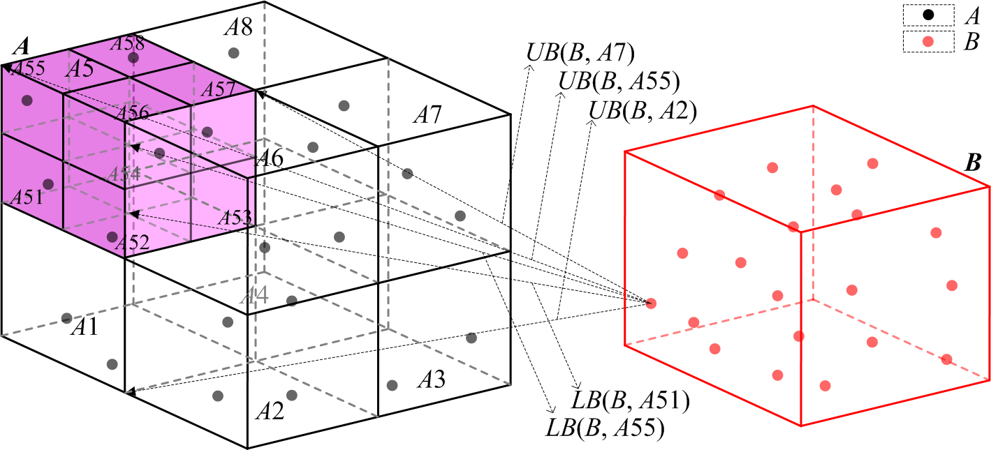
In processing OctreeA, the NOHD algorithm traverse the child node of current node and insert it into DPQ when the UB(B, C) is over MaxLB. Once a UB(B, C) below MaxLB occurs, the traverse on child node of current node will end and the pruning strategy will be executed. For example, if LB(B, A55) is the latest MaxLB, the nodes A2 and A7 are pruned away because UB(B, A2) and UB(B, A7) are less than LB(B, A55). Therefore, MaxLB is constantly updated and the nodes of no-contribution are also pruned away constantly, and finally the Hausdorff distance is obtained.

Figure 5.

Hausdorff distance computation between overlapping point sets.

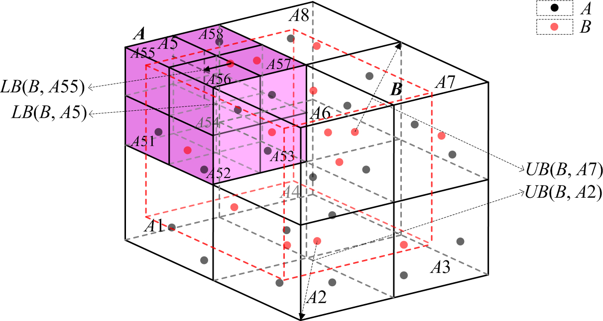
Figure 5 shows a situation, in which A and B are highly overlapping in 3D space. According to analysis in previous Sections, there is no efficient solutions (including the EARLYBREAK algorithm in reference [65] and NOHD algorithm in this manuscript) in this situation for two reasons.

• Firstly, along with the increment of Octree depth, the lower bound from B to most nodes of OctreeA is zero (e.g., LB(B, A5)). Therefore, MaxLB (with zero as the minimum distance) cannot be updated because the upper bound of B to most nodes in OctreeA is over MaxLB, and the pruning strategy cannot be executed in Algorithms 3 and 4.
• Secondly, when A and B are highly similar (e.g., small h(A,B)), the strategy of early breaking in Algorithm 5 will fail in most cases.

Based on the above analysis, both the EARLYBREAK algorithm and NOHD algorithm cannot efficiently reduce the time complexity in overlap situation. Therefore, we proposed the second subalgorithm, the OHD algorithm, to deal with this situation.

4.4The second subalgorithm: OHD

The OHD algorithm computes the Hausdorff distance between A and OctreeB (constructed from B), while NOHD algorithm calculates the Hausdorff distance from OctreeA (constructed from A) to B.

Since the lower bound of the Hausdorff distance between any point ak in A and any node N in OctreeB is 𝑙𝑏⁢(ak,N), the distance between ak and the nearest node in OctreeB is Minlb, where 𝑀𝑖𝑛𝑙𝑏=𝑀𝐼𝑁⁢{𝑙𝑏⁢(ak,N)|N∈𝑂𝑐𝑡𝑟𝑒𝑒B}.

By constantly traveling A and updating Minlb, the maximum Minlb is found (e.g., h⁢(A,B)). In this way, the h(A,B) can be found without traversing all points in A in OHD algorithm, as shown in Algorithm 6.

Algorithm 6. OHD algorithm

Input: Two point set A, BOutput: Directed Hausdorff distance

1. Initialize the AHD
2. Create the OctreeB with the given resolution
(AHD)
3. Maxlb←AHD
4. for each point x of Ado
5. if Point culling ==false then
6. Minlb← NNDist(x, OctreeB)
7. Maxlb←max⁡{𝑀𝑎𝑥𝑙𝑏,𝑀𝑖𝑛𝑙𝑏}
8. end if
9. end for
10. returnMaxLB

The key steps of Algorithm 6 is organized as follows.

• Firstly, the Approximate Hausdorff Distance (AHD) between A and B is Initialized.
• Secondly, an OctreeB for B is built with the given resolution (AHD).
• Thirdly, a strategy of point culling is applied, where any point in A will be culled if it has no contribution to the final Hausdorff distance.
• Finally, the distance between the candidate point and the nearest point in OctreeB is calculated as Minlb, which is used to update current Maxlb if it is greater than the Maxlb. The final Hausdorff distance is the Maxlb at end of the loop.

4.4.1Initialization of Approximate Hausdorff Distance (AHD)

In typical approximate algorithm [65], the initial value of AHD is zero at the time when the outer loop is started. With the gradual execution of outer loop, AHD will monotonically increase and reach the value near to final Hausdorff distance after limited times of the loop.

Therefore, the initialization of AHD can be quickly implemented after limited number of loops, which is set as λ×|A| in OHD algorithm. According our experiment research, this manuscript gives the recommendation as follows: the λ= 1/100.

4.4.2Point culling to reduce number of out iterations for exact algorithm

A strategy of point culling is proposed to reduce number of out iterations, that is, to reduce the point number of A to be traversed in outer loop.

An Octree OctreeB with the given resolution (AHD) is built as shown in Fig. 6, where the cube legends represent leaf nodes of OctreeB, and the red point legends represent A and the black point legends represent B.

Figure 6.

Strategy of point culling.

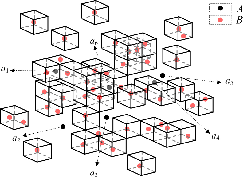
The points of A can be divided into two classes: the leaf-node points and the non-leaf-node points.

• The leaf-node points (such as: a1,a4,a6) are spatially located inside the leaf node of OctreeB, and the temporary Hausdorff distance generated by these points cannot be over AHD and can be safely culled away.
• The non-leaf-node points (such as: a2,⁢a3,⁢a5) are not located in the leaf node of OctreeB, and the temporary Hausdorff distance generated by these points may be over AHD. Therefore, only these points are remained to be further processed by the OHD algorithm.

Therefore, our strategy in OHD algorithm is to cull these leaf-node points.

4.4.3The branch-and-bound and the nearest neighbors distance

The lower bound of the Hausdorff distance between any point ak in A and any node N in OctreeB is 𝑙𝑏⁢(ak,N), so the distance between ak and the nearest node in OctreeB is 𝑀𝑖𝑛𝑙𝑏=𝑀𝐼𝑁⁢{𝑙𝑏⁢(ak,N)|N∈𝑂𝑐𝑡𝑟𝑒𝑒B}. By constantly traveling A and updating of Minlb, the maximum Minlb is found (e.g., h⁢(A,B)).

In order to efficiently reduce number of inner iterations, that is, to avoid traversing all of nodes in OctreeB in inner loop, the OHD algorithm enhances the existing branch-and-bound approach with a new concept of entry of Ascending Priority Queue (APQ). In context of this manuscript, the definition for entry of APQ is given as follows.

Definition 6. Entry(N, Minlb). Attributes of each Entry(N, Minlb) are described as follows: (i) Node N← node in an Octree for B, which could be an object or a non-object(index node); (ii) Distance Minlb← the lower bound of point x of A to node N, that is, lb(x,N).

Where, the APQ arranges Entries(N, Minlb) in ascending order according to the key value Minlb.

The NNDist algorithm is shown as Algorithm 7. The initialization (1 ∼ 3 lines) consists of the following steps: (i) initialize Minlb to ∞; (ii) create a priority queue APQ; (iii) insert the root of OctreeB with an initial Minlb of 0 into APQ.

After the initialization, APQ contains a single entry with the root of OctreeB as the associated node. For each iteration of the while loop (4 ∼ 25 lines), the head Entry(N, lb(ak, N)) is dequeued from APQ. There are two cases depending on whether N is an object or not.

Case 1:

Case 1: If N is not a point object (7 ∼15 lines), two culling procedures are performed.
- – The first culling is based on whether lb(ak, N) from ak to N is less than Minlb or not: if lb(ak, N)⩾Minlb, node N cannot generate a distance less than the current Minlb, and thus should be pruned away; if lb(ak, N)<Minlb, all child nodes in node N should be traversed (8∼13 lines).
- – The second culling is based on whether lb(ak, C) from ak to child node C is over Minlb or not: if lb(ak, C)⩾Minlb, child node C cannot generate a distance less than the current Minlb, and it should be pruned away; if lb(ak, C)<Minlb, child node C may be generate a distance less than the current Minlb, and node C is inserted into APQ.
Case 2: If N is a point object (17 ∼ 23 lines), all points of current node will be processed.
- – First, the distance d from ak to points confined by N is computed.
- – Second, if d is below Maxlb, the ak cannot contribute to the final Hausdorff distance, the APQ is cleared.
- – Third, after comparing d with Minlb, the smaller one is Minlb.

Algorithm 7.NNDist(ak, OctreeB)

Input: Two finite point set A, B;MaxlbOutput:Minlb

1. Minlb←∞
2. APQ← Create an “ascending order”
priority queue
3. Insert(((RootOf(OctreeB), 0), APQ)
4. While (APQ is not empty) do
5. Entry(N, lb(ak, N)← Dequeue(APQ)
6. ifN is non-object then
7. if𝑙𝑏⁢(ak,N)⩽Minlbthen
8. for each child node C of Ndo
9. lb(ak, C)← PointToCube(ak, C)
10. iflb(ak, C)⩽Minlbthen
11. Insert ((C, lb(ak, C), APQ)
12. end if
13. end for
14. end if
15. Sort APQ in ascending order using the
second element
16. else
17. for each point y of Ndo
18. d←∥ak,y∥
19. ifd⩽Maxlbthen
20. APQ←Φ
21. end if
22. Minlb←min⁢{𝑀𝑖𝑛𝑙𝑏,d)
23. end for
24. end if
25. end while

5.An efficient framework based on spatial relationship

Based on spatial relationships of A and B, an efficient framework was proposed, as illustrated in Algorithm 8. Given the degree of overlap between a pair of point sets, the Algorithm 8 choose suitable subalgorithm to compute Hausdorff distance in a way of high efficiency and balance.

As shown in Fig. 7, the Hausdorff distance between A and B is continuously changing from nonoverlapping to fully overlapping.

Algorithm 8. The pseudocode of the proposed framework

Input: Two finite point set A, BOutput: Hausdorff distance

1. Evaluate the space relationship
2. ifA∩B==Φthen
3. Execute the NOHD algorithm
4. else if0⩽α⩽θthen
5. Execute the EARLYBREAK algorithm
6. else
7. Execute the OHD algorithm
8. end if
9. return Hausdorff distance

Figure 7.

The spatial distance between A and B is changing continuously from nonoverlapping to overlapping.

When A∩B=Φ, the NOHD algorithm can efficiently reduce the Octree traversal cost by the strategies of branch-and-bound and early breaking, so the efficiency of the NOHD algorithm is higher than the EARLYBREAK algorithm. Therefore, in our algorithm framework, the NOHD algorithm was employed to compute the Hausdorff distance in this situation.

When A∩B≠Φ (A and B is overlapping as described in Section 4), two algorithms will be called respectively based on the degree of overlap in our algorithm framework. We describe the degree of overlap with α, where 0 ⩽α⩽ 1:

• α is 0 when A and B are just contact;
• α is 1 when A and B are fully overlapping.

We also introduce a threshold θ, which is recommended as 0.33 based on experiments in this manuscript. There are two cases based on the value of threshold θ in our algorithm framework.

• When θ⩽α⩽ 1, the OHD algorithm excludes a large number of points in A that have made no contribution to the final Hausdorff distance. So the efficiency of the OHD algorithm is higher than the EARLYBREAK algorithm. Therefore, the OHD algorithm was employed to compute the Hausdorff distance in this situation.
• When 0 ⩽α⩽θ, only a few points can be excluded by the OHD algorithm, so the efficiency of the OHD algorithm is lower than the EARLYBREAK algorithm. Therefore, the EARLYBREAK algorithm was employed to compute the Hausdorff distance in this situation.

Besides the adaptively and balance, the proposed algorithm can calculate the Hausdorff distance efficiently for general 3D model with an exact result. Under the background, any new and efficient algorithm in future can be easy integrated into the framework, just as the EARLYBREAK algorithm.

6.Experimental results

A number of experiments are conducted to verify the efficiency and effectiveness of the proposed algorithm, which is implemented using on Windows 7/Inter(R) core(TM) i7-4470 (3.4 GHz)/8.00 GB of memory with C+⁣+.

We used the code from the PCL-1.6.0 (http://www. pointclouds.org/) [60] for building Octree. To evaluate the performance of the proposed algorithm, it was tested with three different types of data, namely random 3D Gaussians, point cloud models and CAD/CAE models generated from CAD software.

• In the first experiment (Section 6.1), 3D point sets were generated based on random Gaussians and were used to test the effectiveness of the early breaking strategy for Octree in the NOHD algorithm.
• In the second experiment (Section 6.2), 3D point sets were generated based on random Gaussians and were used to test the effectiveness of the point culling strategy in the OHD algorithm.
• In the third experiment (Section 6.3), 3D point sets were used to test the effect of depth on the efficiency of the NOHD algorithm and the effect of coefficient λ on the efficiency of OHD algorithm.
• In the fourth experiment (Section 6.4), 3D models generated from CAD software were used to compare the proposed algorithm with the EARLYBREAK algorithm under Motion.
• In the last experiment (Section 6.5), several examples from typical fields (such as point cloud models and CAD/CAE models) are tested among the NAIVEHDD algorithm, the INC algorithm, the EARLYBREAK algorithm and the proposed algorithm.

6.1Test for early breaking in the NOHD algorithm

In order to verify the idea of NOHD early breaking strategy in general, random Gaussians data were used for testing. 300 pairs of nonoverlapping random Gaussian point clouds were generated. The number of points in each pair varies from 3 thousands to 0.3 million. The effectiveness of our early breaking strategy in the NOHD algorithm was tested with different number of points in A and B.

In order to verify the effectiveness of NOHD early breaking strategy, we denoted the algorithm that had removed the early breaking strategy from the NOHD algorithm as the NOHD algorithm.

As shown in Table 1, the fourth column and fifth column report the average of 10 computation results for the NOHD algorithm and the NOHD algorithm, individually. The average time cost increased along with the increase in the number of A and B. However, compared with the NOHD algorithm, the NOHD algorithm can efficiently reduce the average time cost by the early breaking strategy.

Table 1

Contribution of early breaking: Comparison between the efficiency of the NOHD algorithm when using early breaking or not

Pairs	Set size		Execution time (sec)
	\|A\|	\|B\|	NOHD	NOHD
(1)	3 K	3 K	0.03589	0.02247
(2)	15 K	10 K	0.14427	0.09993
(3)	23 K	27 K	0.33513	0.23967
(4)	43 K	41 K	0.45207	0.3058
(5)	49 K	64 K	0.65733	0.3232
(6)	64 K	78 K	0.96393	0.48947
(7)	77 K	51 K	0.58567	0.42353
(8)	86 K	35 K	0.65933	0.58753
(9)	105 K	113 K	1.07733	0.74767
(10)	123 K	31 K	1.14933	0.74567
(11)	131 K	93 K	1.1878	0.70933
(12)	145 K	110 K	1.2986	0.8624
(13)	169 K	160 K	1.5378	0.99287
(14)	210 K	220 K	2.07807	1.34207
(15)	231 K	239 K	2.2312	1.38447

6.2Test for point culling in OHD algorithm

In order to verify the validity of the point culling strategy in the OHD algorithm, the same data sets as Section 6.1 are used. We denoted the algorithm that had removed the point culling strategy from the OHD algorithm as the OHD algorithm.

Table 2

Contribution of point culling: Comparison between the efficiency of the OHD algorithm when using point culling or not

Pairs	Set size		Execution time (sec)
	\|A\|	\|B\|	OHD	OHD
(1)	4 K	4 K	1.577	0.56087
(2)	6 K	12 K	3.1044	1.67333
(3)	8 K	4 K	2.617	0.92533
(4)	12 K	16 K	5.385	2.11597
(5)	21 K	15 K	8.6174	2.04287
(6)	29 K	24 K	12.07487	5.299
(7)	29 K	17 K	10.78667	3.97227
(8)	37 K	22 K	15.1934	3.6774
(9)	39 K	32 K	17.3132	6.28933
(10)	40 K	34 K	15.83447	5.7202
(11)	40 K	28 K	16.64947	5.48007
(12)	41 K	35 K	20.3706	9.5222
(13)	44 K	26 K	16.0276	4.86627
(14)	46 K	47 K	20.1598	7.574
(15)	51 K	39 K	20.69647	7.33847

As shown in Table 2, the fourth column and fifth column report the average of 10 computation results for the OHD algorithm and the OHD algorithm, individually. The OHD algorithm did not adopt the point culling strategy and Algorithm 7 should be called for each points in A, while the OHD algorithm used the point culling strategy to exclude the points with no contribution to the final Hausdorff distance and Algorithm 7 is called for only part of points in A. Therefore, compared with the OHD algorithm, the OHD algorithm can efficiently reduce the time cost with the point culling strategy.

6.3Analysis of some important parameters

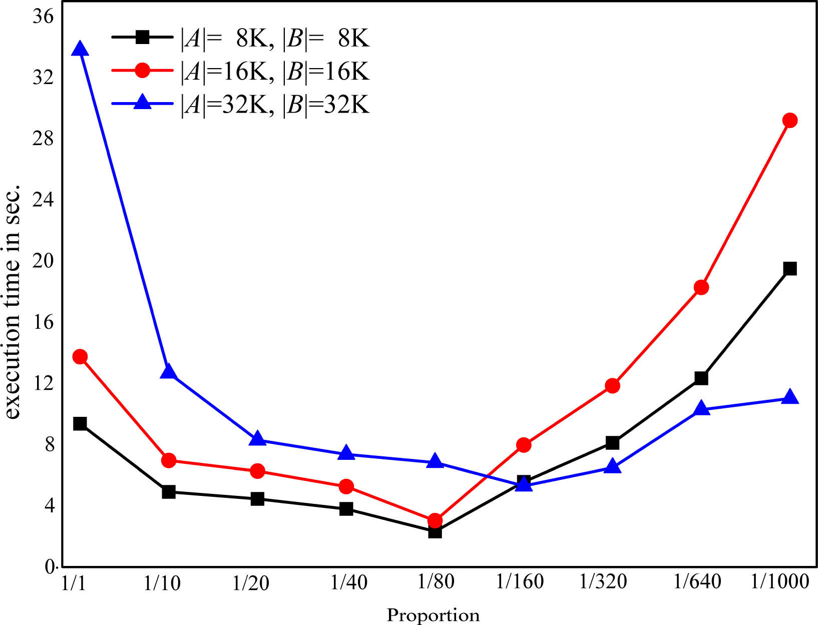
To further analyze various characteristics of the method, we discussed the effect of depth on the efficiency of the NOHD algorithm and the effect of coefficient λ on the efficiency of OHD algorithm.

Figure 8.

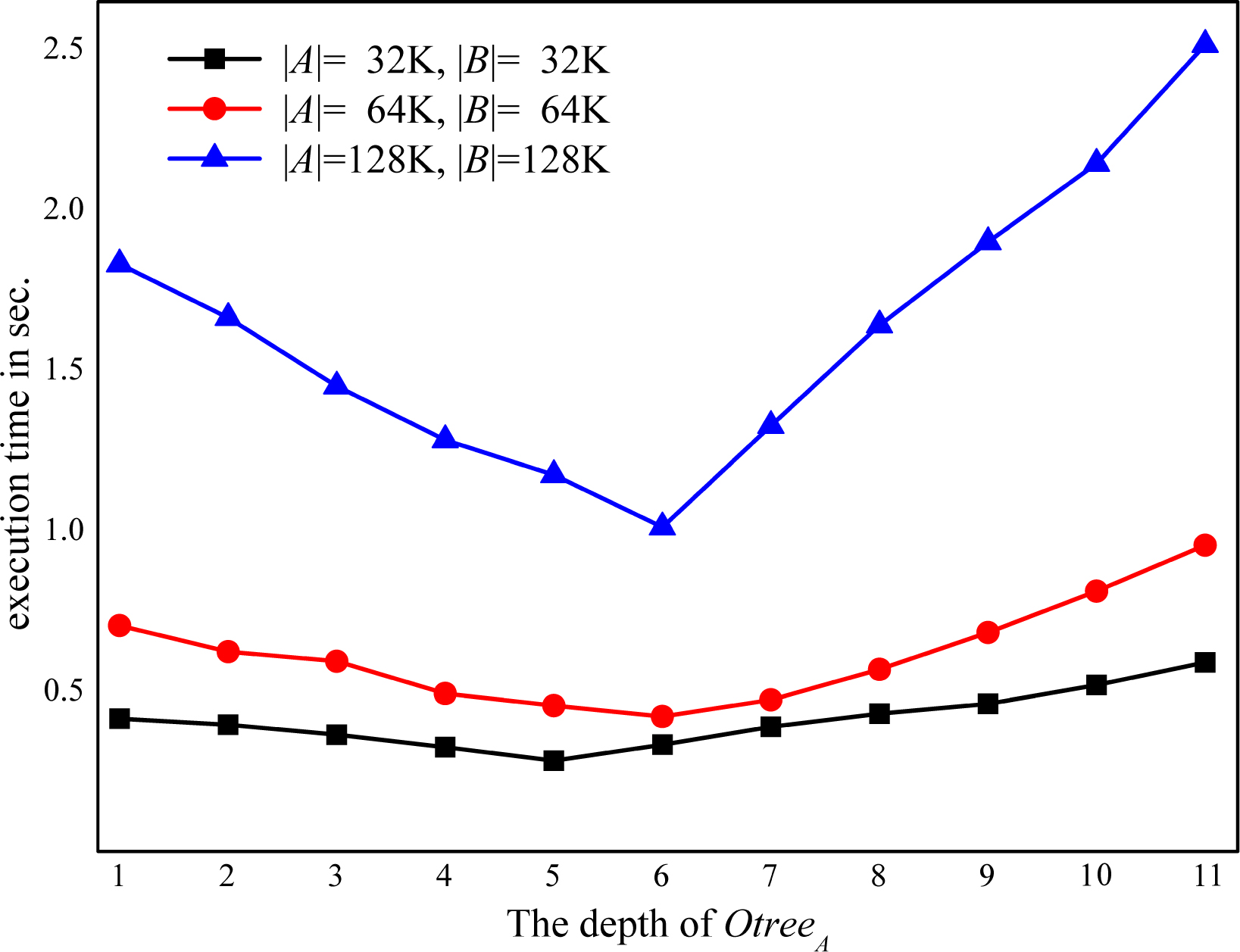
The relationship between depth of OctreeA and execution time of NOHD algorithm.

In context of this manuscript, in the case of spatial nonoverlap, the calculation of Hausdorff distance from A to B is converted into calculating the Hausdorff distance from OctreeA to B.

We need to set the depth of Octree before constructing the OctreeA from A. In general, the time cost of constructing an Octree is proportional to the depth of Octree. We selected three pairs of random Gaussian point clouds to test the effect of depth on the efficiency of the NOHD algorithm. The relationship between the depth and the average execution time from 10 trials is shown in Fig. 8. The efficiency of NOHD algorithm is improved with the increasing of the value of depth, and the high efficiency is obtained when depth is increased to five or six. Moreover, with a bigger value of depth, the efficiency is decreased.

According to the experimental research, this manu- script recommended the depth of six.

Figure 9.

The relationship between λ and execution time of OHD algorithm.

When A and B were highly overlapping, the calculation of Hausdorff distance from A to B is converted into calculating the Hausdorff distance between A and OctreeB.

The OctreeB is built with the given resolution (AHD). In context of this manuscript, the greater the value of AHD is, the more efficiency of the point culling within OHD algorithm is. Thus, the coefficient λ directly effects the value of AHD, and indirectly effects the efficiency of computing the Hausdorff distance by OHD algorithm. We selected three pairs of random Gaussian point clouds to test the effect of coefficient λ on the efficiency of the OHD algorithm. The relationship between the coefficient λ and the average execution time from 10 trials is shown in Fig. 9. The efficiency of OHD algorithm is improved with the decreasing of λ, and the high efficiency is obtained when λ is set as 1/80. Moreover, with a smaller value of λ, the efficiency is decreased as a result of that the AHD is much less than the Hausdorff distance.

According to our experimental research, this manu- script gives the recommendation as follows: the λ= 1/100.

6.4Hausdorff distance under motion

An important variation of the Hausdorff distance problem is to find the distance when there is a relative movement between two models, such as penetration [66, 73]. This problem is known as geometric matching under the Hausdorff distance metric. In this section, we computed the Hausdorff distance between a fixed model and a moving model to fully illustrate the efficiency of the proposed algorithm.

Two models M and M′ with same shape and same size are shown in Fig. 10(a). As demonstrated in Fig. 10(b), with the decrease in the Hausdorff distance, the average time cost gradually increased. When M and M′ were highly overlapping, the time cost reached the peak value. With the increase in the Hausdorff distance, the time cost gradually decreased.

Figure 10.

HD computation between a stationary torus and a moving torus. (a) One torus is moving under a continuous translation. (b) Comparison of the execution time between the proposed algorithm and the EARLYBREAK algorithm.

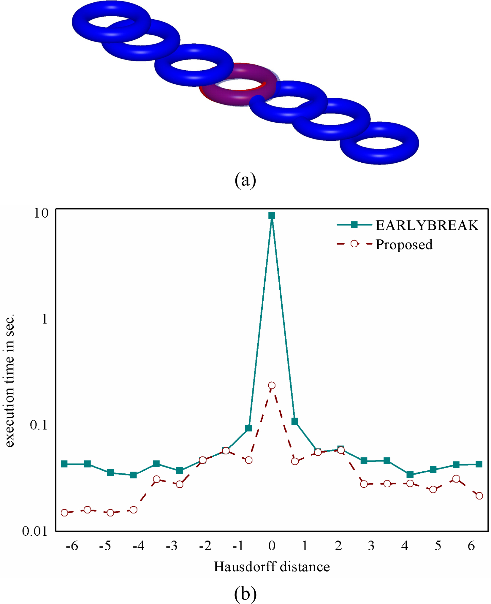
When two models were nonoverlapping, the average time cost of the NOHD algorithm was significantly better than that of the EARLYBREAK algorithm. When the degree of overlap fell into the range of 0 ⩽α⩽ 0.33, the EARLYBREAK algorithm was integrated into our algorithm framework. When the degree of overlap fell into the range of 0.33 ⩽α⩽ 1, the time cost of the OHD algorithm was significantly better than that of the EARLYBREAK algorithm.

As shown in Fig. 11, although two models are tested with different shape and size, the proposed algorithm achieved the same result as above.

6.5Point cloud models and CAD/CAE/CAM models

In order to further evaluate its performance, the proposed approach was applied to several examples from different fields (such as point cloud models and CAD/ CAE/CAM models) for experimental comparison.

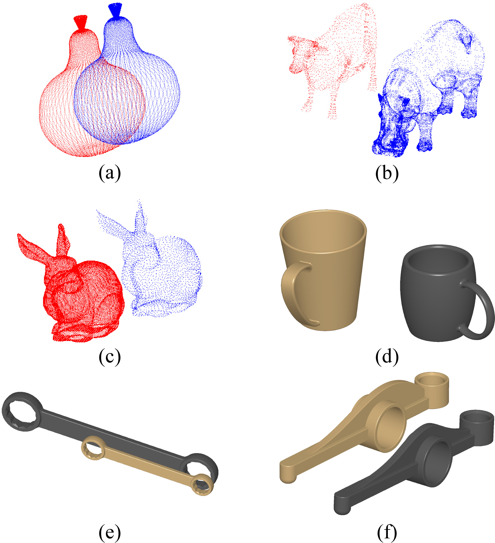
Three pairs of point cloud models and three pairs of CAD/CAE/CAM models were tested in this section as shown in Fig. 12. The step of calculating the Hausdorff distance between the models was as follows: (1) Models M and M′ were converted point sets A and B; (2) the Hausdorff distance was calculated by Eqs (1)–(3).

Table 3

Hausdorff distance computation for different cases

Index	Execution time (sec)
	NAIVEHDD	INC	EARLYBREAK	PROPOSED
(a)	47.282	3.107	0.226	0.225
(b)	27.782	2.013	0.363	0.091
(c)	51.933	21.07	6.658	2.136
(d)	39.936	0.722	0.109	0.051
(e)	11.371	0.828	0.062	0.063
(f)	92.576	50.044	5.381	0.531

Figure 11.

HD computation between a stationary gear and a moving gear. (a) One gear is moving under a continuous translation and rotation. (b) Comparison of the execution time between the proposed algorithm and the EARLYBREAK algorithm.

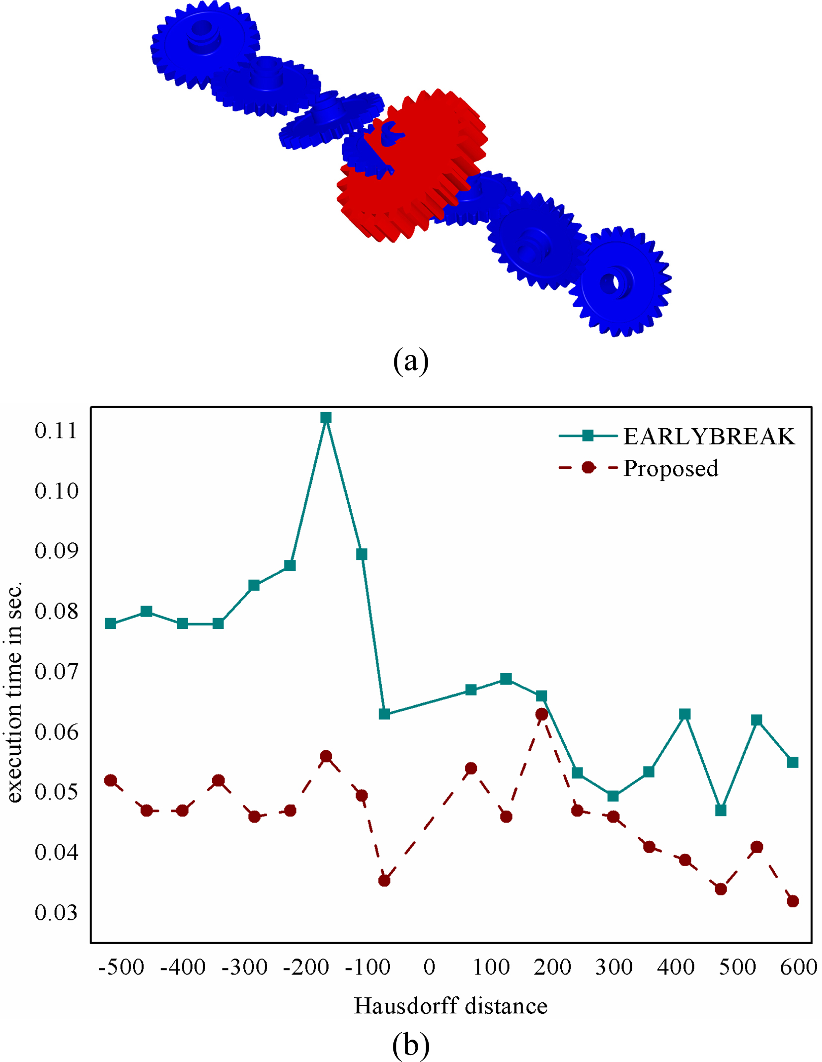
Figure 12.

The different cases used for timing the minimum distance computations: (a) pears (10,754–10,754); (b) cow and hippo (2,903–23,105); (c) two rabbits with different resolution (34,834–3,594); (d) different cups (10,007–9,449); (e) different wrenches (5,191–5,290); (f) singular models (13,564–12,680).

The time costs in calculating the Hausdorff distance through the NAIVEHDD algorithm, the incremental Hausdorff distance calculation algorithm (INC) [54], the EARLYBREAK algorithm [65], and the proposed algorithm were shown in Table 3 (The units of time is second).

According to the comparison of experiments, the time cost executed by the proposed algorithm in calculating the Hausdorff distance is significantly less than that executed by the NAIVEHDD algorithm, and is distinctly less than that executed by the EARLYBREAK algorithm.

The proposed algorithm is composed of the NOHD, the OHD and the EARLYBREAK algorithm. The NOHD algorithm combines branch-and-bound with early breaking to cut down the Octree traversal time in case of spatial nonoverlap. The OHD algorithm integrates a point culling strategy and nearest neighbor search to reduce the number of points traversed in case of spatial overlap.

Therefore, the high efficiency of the NOHD algorithm and the OHD algorithm in the proposed efficient framework was confirmed once again.

7.Conclusion and future work

An efficient framework with two complementary subalgorithms is presented with theory analysis. The experiments also demonstrate that the proposed approach, as a whole, outperforms the state-of-the art algorithms [54, 65]. The main contributions are summarized as follows:

(1)

(1) Besides individual algorithms, an efficient framework is presented, which automatically chooses the suitable subalgorithms to compute the Hausdorff distance in different spatial relationship between a pair of point sets. In this way, the long-standing limitation of computing Hausdorff distance can be relaxed.
(2) In NOHD algorithm, we present a strategy synthesizing branch-and-bound and early breaking, and efficiently reduce cost of the Octree traversal. In OHD algorithm, we construct a strategy combining point culling and nearest neighbor searching, and efficiently reduces the cost of points traverse. And different from the state-of-the art algorithm [54, 65], the proposed algorithms can directly calculate a pair of the 3D point sets without transforming them into voxel model.
(3) The experiments demonstrate that the proposed approach, as a whole, outperforms the state-of-the art algorithms [65].
(4) The proposed framework can easily integrate other algorithms. Therefore, any subalgorithm with a high efficiency can be added into this framework in the future.

Since distance measurement is fundamental operation in applications of science, engineering and industry [15, 21, 43, 50, 53, 56, 64, 71, 74, 75, 76], we will explore following directions but no limited in future work:

(1)

(1) The qualitative evaluation of model similarity, such as similarity assessments for 3D CAD/ CAE model retrieval [10, 17], focused on the qualitative aspects of the models, e.g., topological result and geometric profile. On the other hand, in the field of data exchange [29, 37, 42, 51, 57, 58, 67, 69] and collaborative design [19, 20, 33, 44, 45, 49], the quantitative comparison of the similarity between source and target of feature-based CAD models is the latest development [72]. So the proposed method can be adopted in this area to improve the computing efficiency of quantitative comparisons between large scale models in engineering applications of CAD/CAE/CAM in the future. For example, the proposed algorithms can enhance the computing efficiency of quantitative comparisons in Feature-based Data Exchange in CAD/CAE/CAM when calculating the fitness in optimization computation [72].
(2) This work is also related with design automation because the exact Hausdorff distance will be automatically computed. Design automation is considered as a particularly challenging issue in Computer-Aided Engineering systems, such as A MICROCAD system for interactive design of connections in steel buildings engineering [1, 2], object-oriented model-based presentation for integrated design of steel buildings structures [3, 4], and so on.
(3) The multi-core CPUs and many-core GPUs are nice choices for high-performance, low-power and cost-sensitive industrial applications. And they are also available on common PC platforms. Therefore, from view of practice, we should try improve our algorithm with multi-core/many-core acceleration platforms for industrial applications [14, 27, 77, 78].

Acknowledgments

This work is supported by the National Science Foundation of China (Grant No. 61472289) and Open Project Program of State Key Laboratory of Digital Manufacturing Equipment and Technology at HUST (Grant No. DMETKF2017016).

References

[1]	Adeli H, Fiedorek J. A MICROCAD system for design of steel connections-applications. Comput & Struct. (1986) ; 24: (3): 361-374.
[2]	Adeli H, Fiedorek J. A MICROCAD system for design of steel connections-program structure and graphic algorithms. Comput & Struct. (1986) ; 24: (2): 281-294.
[3]	Adeli H, Kao WM. Object-oriented blackboard models for integrated design of steel structures. Comput & Struct. (1996) ; 61: (3): 545-561.
[4]	Adeli H, Yu G. An integrated computing environment for solution of complex engineering problems using the object-oriented programming paradigm and a blackboard architecture. Comput & Struct. (1995) ; 54: (2): 255-265.
[5]	Alt H, Behrends B, Blömer J. Approximate matching of polygonal shapes. Ann Math Artif Intel. (1995) ; 13: (3-4): 251-265.
[6]	Alt H, Braß P, Godau M, Knauer C, Wenk C. Computing the Hausdorff distance of geometric patterns and shapes. Discret Comput Geom. (2003) ; 65-76.
[7]	Alt H, Scharf L. Computing the Hausdorff distance between curved objects. Int J Comput Geom Ap. (2008) ; 18: (4): 307-320.
[8]	Aspert N, Santa Cruz D, Ebrahimi T. MESH: Measuring errors between surfaces using the Hausdorff distance. ICME. (2002) ; 705-708.
[9]	Atallah MJ. A linear time algorithm for the Hausdorff distance between convex polygons. Inform Process Lett. (1983) ; 17: (4): 207-209.
[10]	Bai J, Gao S, Tang W, Liu Y, Guo S. Design reuse oriented partial retrieval of CAD models. Comput Aided Design. (2010) ; 42: (12): 1069-1084.
[11]	Bai YB, Yong JH, Liu CY, Liu XM, Meng, Y. Polyline approach for approximating Hausdorff distance between planar free-form curves. Comput Aided Design. (2011) ; 43: (6): 687-698.
[12]	Bartoň M. Solving polynomial systems using no-root elimination blending schemes. Comput Aided Design. (2011) ; 43: (12): 1870-1878.
[13]	Bartoň M, Hanniel I, Elber G, Kim MS. Precise Hausdorff distance computation between polygonal meshes. Comput Aided Geom D. (2010) ; 27: (8): 580-591.
[14]	Belloch JA, Gonzalez A, Martinez-Zaldivar FJ, Vidal AM. Multichannel massive audio processing for a generalized crosstalk cancellation and equalization application using GPUs. Integr Comput-Aid E. (2013) ; 20: (2): 169-182.
[15]	Bi ZM, Wang L. Advances in 3D data acquisition and processing for industrial applications. Robot Cim-Int Manuf. (2010) ; 26: (5): 403-413.
[16]	Cardone A, Gupta SK, Deshmukh A, Karnik M. Machining feature-based similarity assessment algorithms for prismatic machined parts. Comput Aided Design. (2006) ; 38: (9): 954-972.
[17]	Chen X, Gao S, Guo S, Bai J. A flexible assembly retrieval approach for model reuse. Comput Aided Design. (2012) ; 44: (6): 554-574.
[18]	Chen XD, Ma W, Xu G, Paul JC. Computing the Hausdorff distance between two B-spline curves. Comput Aided Design. (2010) ; 42: (12): 1197-1206.
[19]	Cheng Y, He F, Cai X, Zhang D. A group Undo/Redo method in 3D collaborative modeling systems with performance evalua-tion. J Netw Comput Appl. (2013) ; 36: (6): 1512-1522.
[20]	Cheng Y, He F, Wu Y, Zhang D. Meta-operation Conflict Resolution for Human-Human Interaction in Collaborative Feature-Based CAD systems. Cluster Comput. (2016) ; 19: (1): 237-253.
[21]	Cheng HC, Lo CH, Chu CH, Kim YS. Shape similarity measurement for 3D mechanical part using D2 shape distribution and negative feature decomposition. Comput Ind. (2011) ; 62: (3): 269-280.
[22]	Cignoni P, Rocchini C, Scopigno R. Metro: measuring error on simplified surfaces. Comput Graph Forum. (1998) ; 17: (2): 167-174.
[23]	Dubuisson MP, Jain AK. A modified Hausdorff distance for object matching. Pattern Recognition. 12th IAPR International Conference. (1994) ; 1: : 566-568.
[24]	Fukunaga K, Narendra PM. A branch and bound algorithm for computing k-nearest neighbors. Ieee T Comput. (1975) ; 100: (7): 750-753.
[25]	Guo B, Lam KM, Lin KH, Siu WC. Human face recognition based on spatially weighted Hausdorff distance. Pattern Recogn Lett. (2003) ; 24: (1): 499-507.
[26]	Guthe M, Borodin P, Klein R. Fast and accurate Hausdorff distance calculation between meshes. International Conferences in Central Europe on Computer Graphics and Visualization. (2005) ; 41-48.
[27]	Guthier B, Kopf S, Wichtlhuber M, Effelsberg W. Parallel implementation of a real-time high dynamic range video system. Integr Comput-Aid E. (2014) ; 21: (2): 189-202.
[28]	Hanniel I, Krishnamurthy A, McMains S. Computing the Hausdorff distance between NURBS surfaces using numerical iteration on the GPU. Graph Models. (2012) ; 74: (4): 255-264.
[29]	Hoffmann C, Shapiro V, Srinivasan V. Geometric interoperability via queries. Comput Aided Design. (2014) ; 46: : 148-159.
[30]	Huttenlocher DP, Kedem K, Kleinberg JM. On dynamic Voronoi diagrams and the minimum Hausdorff distance for point sets under Euclidean motion in the plane. The eighth annual symposium on Computational geometry. (1992) ; 110-119.
[31]	Huttenlocher DP, Klanderman GA, Rucklidge WJ. Comparing images using the Hausdorff distance. Ieee T Pattern Anal. (1993) ; 15: (9): 850-863.
[32]	Hwang CM, Yang MS, Hung WL, Lee M. A similarity measure of intuitionistic fuzzy sets based on the Sugeno integral with its application to pattern recognition. Inform Sciences. (2012) ; 189: : 93-109.
[33]	Jing S, He F, Han S, Cai X, Liu H. A method for topological entity correspondence in a replicated collaborative CAD system. Comput Ind. (2009) ; 60: (7): 467-475.
[34]	Kim YJ, Oh YT, Yoon SH, Kim MS, Elber G. Coons BVH for freeform geometric models. Acm T Graphic. (2011) ; 30: (6): 169.
[35]	Kim YJ, Oh YT, Yoon SH, Kim MS, Elber G. Efficient Hausdorff distance computation for freeform geometric models in close proximity. Comput Aided Design. (2013) ; 45: (2): 270-276.
[36]	Kim YJ, Oh YT, Yoon SH, Kim MS, Elber G. Precise Hausdorff distance computation for planar freeform curves using biarcs and depth buffer. Visual Comput. (2010) ; 26: (6-8): 1007-1016.
[37]	Kim J, Pratt MJ, Iyer RG, Sriram RD. Standardized data exchange of CAD models with design intent. Comput Aided Design. (2008) ; 40: (7): 760-777.
[38]	Krishnamurthy A, McMains S, Halle K. Accelerating geometric queries using the GPU. SIAM/ACM Joint Conference on Geometric and Physical Modeling. (2009) ; 199-210.
[39]	Krishnamurthy A, McMains S, Hanniel I. GPU-accelerated Hausdorff distance computation between dynamic deformable NURBS surfaces. Comput Aided Design. (2011) ; 43: (11): 1370-1379.
[40]	Lertchuwongsa N, Gouiffès M, Zavidovique B. Enhancing a disparity map by color segmentation. Integr Comput-Aid E. (2012) ; 19: (4): 381-397.
[41]	Lertchuwongsa N, Gouiffès M, Zavidovique B. Mixed color/level lines and their stereo-matching with a modified Hausdorff distance. Integr Comput-Aid E. (2011) ; 18: (2): 107-124.
[42]	Li J Kim BC, Han S. Parametric exchange of round shapes between a mechanical CAD system and a ship CAD system. Comput Aided Design. (2012) ; 44: (2): 154-161.
[43]	Li K, He F, Chen X. Real time object tracking via compressive feature selection. Front Comput Sci. (2016) ; 10: (4): 689-701.
[44]	Li WD, Lu WF, Fuh JYH, Wong YS. Collaborative computer-aided design research and development status. Computer-Aided Design. (2005) ; 37: (9): 931-940.
[45]	Li X, He F, Cai X, Zhang D, Chen Y. A method for topological entity matching in the integration of heterogeneous CAD systems. Integr Comput-Aid E. (2013) ; 20: (1): 15-30.
[46]	Lin KH, Lam KM, Siu WC. Spatially eigen-weighted Hausdorff distances for human face recognition. Pattern Recogn. (2003) ; 36: (8): 1827-1834.
[47]	Llanas B. Efficient computation of the Hausdorff distance between polytopes by exterior random covering. Comput Optim Appl. (2005) ; 30: (2): 161-194.
[48]	Lockett H, Guenov M. Similarity measures for mid-surface quality evaluation. Comput Aided Design. (2008) ; 40: (3): 368-380.
[49]	Lv X, He F, Cai W, Cheng Y. A string-wise CRDT algorithm for smart and large-scale collaborative editing systems. Adv Eng Inform. DOI: 10.1016/j.aei.2016.10.005.
[50]	Mohan P, Haghighi P, Vemulapalli P, Kalish N, Shah JJ, Davidson JK. Toward automatic tolerancing of mechanical assemblies: Assembly analyses. J Comput Inf Sci Eng. (2014) ; 14: (4): 041009.
[51]	Mun D, Han S, Kim J, Oh Y. A set of standard modeling commands for the history-based parametric approach. Comput Aided Design. (2003) ; 35: (13): 1171-1179.
[52]	Ni B, He F, Pan Y, Yuan Z. Using shapes correlation for active contour segmentation of uterine fibroid ultrasound images in computer-aided therapy. Appl Math Ser B. (2016) ; 31: (1): 37-52.
[53]	Ni B, He F, Yuan Z. Segmentation of uterine fibroid ultrasound images using a dynamic statistical shape model in HIFU therapy. Comput Med Imag Grap. (2015) ; 46: : 302-314.
[54]	Nutanong S, Jacox EH, Samet H. An incremental Hausdorff distance calculation algorithm. Proceedings of the VLDB Endowment. (2011) ; 4: (8): 506-517.
[55]	Papadias D, Tao Y, Mouratidis K, Hui CK. Aggregate nearest neighbor queries in spatial databases. Acm T Database Syst. (2005) ; 30: (2): 529-576.
[56]	Primerano R, Wilkie D, Regli WC. A case study in system-level physics-based simulation of a biomimetic robot. Ieee T Autom Sci Eng. (2011) ; 8: (3): 664-671.
[57]	Qi J, Shapiro V. Geometric interoperability with epsilon solidity. J Comput Inf Sci Eng. (2006) ; refvol6(3): 213-220.
[58]	Rappoport A. An architecture for universal CAD data exchange. Proceedings of the eighth ACM symposium on Solid modeling and applications. (2003) ; 266-269.
[59]	Rucklidge W. Efficient visual recognition using the Hausdorff distance. Lect Notes Comput Sc. (1996) ; 1173.
[60]	Rusu RB, Cousins S. 3d is here: Point cloud library (pcl). IEEE International Conference on Robotics and Automation. (2011) ; 1-4.
[61]	Sangineto E. Pose and expression independent facial landmark localization using dense-SURF and the Hausdorff distance. Ieee T Pattern Anal. (2013) ; 35: (3): 624-638.
[62]	Sim DG, Kwon OK, Park RH. Object matching algorithms using robust Hausdorff distance measures. Ieee T Image Process. (1999) ; 8: (3): 425-429.
[63]	Sudha N. Robust Hausdorff distance measure for face recognition. Pattern Recogn. (2007) ; 40: (2): 431-442.
[64]	Sun J, He F, Chen Y, Chen X. A multiple template approach for robust tracking of fast motion target. Appl Math Ser B. (2016) ; 31: (2): 177-197.
[65]	Taha AA, Hanbury A. An efficient algorithm for calculating the exact Hausdorff distance. Ieee T Pattern Anal. (2015) ; 37: (11): 2153-2163.
[66]	Tang M, Lee M, Kim YJ. Interactive Hausdorff distance computation for general polygonal models. Acm T Graphic. (2009) ; 28: (3): 1-9.
[67]	Tessier S, Wang Y. Ontology-based feature mapping and verification between CAD systems. Adv Eng Inform. (2013) ; 27: (1): 76-92.
[68]	Wu Y, He F, Han S. Collaborative CAD synchronization based on a symmetric and consistent modeling procedure. Symmetry. (2017) ; 9: (4): 59.
[69]	Wu Y, He F, Zhang D, Li X. Service-oriented feature-based data exchange for cloud-based design and manufacturing. Ieee T Serv Comput. DOI: 10.1109/TSC.2015.2501981.
[70]	Yu H, He F, Pan Y, Chen X. An efficient similarity-based level set model for medical image segmentation. J Adv Mech Des Syst Manuf. (2016) ; 10: (8): JAMDSM0100.
[71]	Zeng Y, HorváTh I. Fundamentals of next generation CAD/E systems. Comput Aided Design. (2012) ; 44: (10): 875-878.
[72]	Zhang DJ, He FZ, Han SH, Li XX. Quantitative optimization of interoperability during feature-based data exchange. Integr Comput-Aid E. (2016) ; 23: (1): 31-51.
[73]	Zhang L, Kim YJ, Varadhan G, Manocha D. Generalized penetration depth computation. Comput Aided Design. (2007) ; 39: (8): 625-638.
[74]	Yan X, He F, Chen Y, Yuan Z. An efficient improved particle swarm optimization based on prey behavior of fish schooling. J Adv Mech Des Syst Manuf. (2015) ; 9: (4): JAMDSM0048.
[75]	Yan X, He F, Hou N. A novel hardware/software partitioning method based on position disturbed particle swarm optimization with invasive weed optimization. J Comput Sci Tech. (2017) ; 32: (2): 340-355.
[76]	Yan X, He F, Hou N, Ai H. An efficient particle swarm optimization for large scale hardware/software co-design system. Int J Coop Inf Syst. DOI: S0218843017410015.
[77]	Zhou Y, He F, Qiu Y. Dynamic strategy based parallel ant colony optimization on GPUs for TSPs. Sci China Inform Sci. (2017) ; 60: : 068102.
[78]	Zhou Y, He F, Qiu Y. Optimization of parallel iterated local search algorithms on graphics processing unit. J Supercomput. (2016) ; 72: (6): 2394-2416.

Abstract

1.Introduction

2.Related work

2.1Curves and surfaces

2.2Polygonal models

2.3Point sets

3.Problem state

3.1Hausdorff distance

(1)

(2)

(3)

3.2NAIVEHDD and one-side BREAK algorithm

3.3Challenge and analysis

(4)

(5)

(6)

(7)

Figure 1.

4.The proposed two subalgorithms

4.1The definition of bound and the description of overlap

(8)

(9)

Figure 2.

(10)

(11)

(12)

(13)

(14)

Figure 3.

4.2The first subalgorithm: NOHD

4.2.1The basic idea of NOHD and the definition of priority queue

4.2.2NOHD algorithm description

4.3Difficulties for computing hausdorff distance in overlap situation

Figure 4.

Figure 5.

4.4The second subalgorithm: OHD

4.4.1Initialization of Approximate Hausdorff Distance (AHD)

4.4.2Point culling to reduce number of out iterations for exact algorithm

Figure 6.

4.4.3The branch-and-bound and the nearest neighbors distance

Case 1:

5.An efficient framework based on spatial relationship

Figure 7.

6.Experimental results

6.1Test for early breaking in the NOHD algorithm

Table 1

6.2Test for point culling in OHD algorithm

Table 2

6.3Analysis of some important parameters

Figure 8.

Figure 9.

6.4Hausdorff distance under motion

Figure 10.

6.5Point cloud models and CAD/CAE/CAM models

Table 3

Figure 11.

Figure 12.

7.Conclusion and future work

(1)

(1)

Acknowledgments

References

Share this:

North America

Europe

Asia