Vehicle side-slip angle estimation under snowy conditions using machine learning
Abstract
Adverse weather conditions, such as snow-covered roads, represent a challenge for autonomous vehicle research. This is particularly challenging as it might cause misalignment between the longitudinal axis of the vehicle and the actual direction of travel. In this paper, we extend previous work in the field of autonomous vehicles on snow-covered roads and present a novel approach for side-slip angle estimation that combines perception with a hybrid artificial neural network pushing the prediction horizon beyond existing approaches. We exploited the feature extraction capabilities of convolutional neural networks and the dynamic time series relationship learning capabilities of gated recurrent units and combined them with a motion model to estimate the side-slip angle. Subsequently, we evaluated the model using the 3DCoAutoSim simulation platform, where we designed a suitable simulation environment with snowfall, friction, and car tracks in snow. The results revealed that our approach outperforms the baseline model for prediction horizons
1.Introduction
Novel safety systems which control vehicle dynamics monitor key sensor signals such as wheel angular velocities, steering angle, yaw rate, and vehicle side-slip angle [1]. The side-slip angle, also known as drift or attitude, represents the misalignment between the vehicle’s longitudinal axis and its travel direction, making it crucial for systems like ESC to ensure safety. Vehicle control systems including the ESC, active steering, and ATC rely on real-time vehicle state assessments, particularly the VSA [2, 3]. The vehicle’s state comprises longitudinal and lateral velocity or acceleration, steering angle, yaw rate, and more. These properties can be measured directly (like acceleration, steering angle) or inferred from sensor data. However, calculating the VSA is complex as it depends on wheel and ground friction, wheel forces, and vehicle dynamics [2, 3, 4]. Determining these factors directly is costly and complicated, requiring high-precision sensors [5, 2, 3, 4, 6, 7]. Therefore, researchers have long investigated VSA estimation methods, starting as early as 1990 [2]. This study primarily employs an empirical descriptive model to explore and confirm the relationships between vehicle and road factors and VSA. To ensure a comprehensive understanding of these relationships, we have employed statistical analyses using both Spearman and Pearson correlation methods, allowing us to analyze the data in multiple dimensions. As indicated in [5], the vehicle maneuverability strongly depends on the size of the VSA. Under dry road conditions the vehicle can achieve a VSA of up to ten degrees. However, in snowy conditions, this value is limited to a maximum of four degrees to ensure the vehicle remains maneuverable.
Figure 1.
Top view of a vehicle during a right turn, with a fixed coordinate frame at
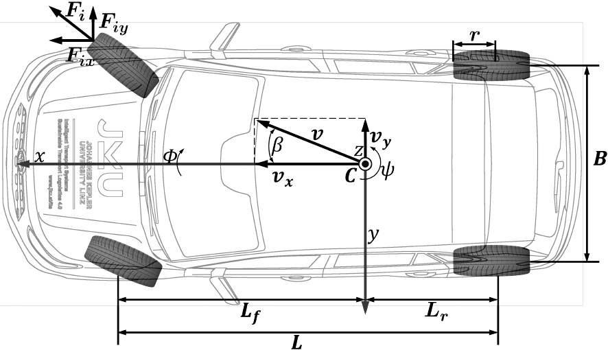
Typically, when estimating the VSA, the physical properties depicted in Fig. 1 are taken into account. These properties are either provided by (CAN) BUS data or acquired through proprioceptive sensors. In the following, we aim to provide a wide baseline for understanding the performance of various VSA estimate methodologies, particularly under diverse situations, and according to [2, 3, 8, 9], these approaches can be primarily classified as:
• Observer – based: These approaches rely either on a kinematic or dynamic model of the vehicle in combination with an observer, where the most common ones are derivatives of the bayes filter, such as KF and its non-linear derivatives EKF and UKF.
• Neural Network – based: Most approaches rely on the same NN structure consisting of a total of three layers composed of one input layer, one fully connected hidden layer with log-sigmoid activation, and one output layer with linear activation.
The issue of estimating the VSA becomes particularly relevant under non-optimal weather conditions such as cases involving snow-covered roadways, as described in [10]. As observer-based estimators drastically rely on models of not only the vehicle but also of the tire-road interaction, the performance of these varies according to the accuracy of the model as well as the sensor systems utilized. Moreover, the non-linear characteristics of driving make it difficult to obtain a satisfactory model and estimation performance.
The findings presented in [3] elucidate several points on vehicle dynamics. Dynamic-based observer methods apply effectively only at
In [4] four different NN estimators for VSA estimation were compared: FFNN [11], RNN [12], GRU [13], and LSTM [14]. These networks were compared in terms of accuracy based on the RMSE, mean training time, and mean estimation time. They concluded that FFNN achieved the highest accuracy and lowest estimation time but also the highest training time. LSTM outperformed GRU in terms of accuracy, but took longer for each prediction and overall training.
As stated at the beginning of this section, accurate estimation of the VSA is crucial for efficient ESC, which in turn can significantly mitigate vehicle spinning – a primary contributor to nearly 25% of human-injury-related accidents [4].
Prompted by this necessity, we contribute to the state of the art in VSA estimation, by proposing an enhanced sensor configuration and a novel approach to integrate sensor data for more precise estimation over an extended prediction horizon.
We present a model for estimating VSA on snowy roads – a challenging scenario for ESC systems [5]. Building on the premise that exteroceptive sensor data, strictly speaking visual characteristics, can enhance prediction accuracy [15, 16], we introduce an approach that integrates image features extracted by a CNN [17] into a hybrid artificial neural network [8]. This method leverages the rich visual cues from CNN-processed camera feeds, thereby uncovering previously unexplored VSA-related information and improving prediction accuracy over existing techniques.
Camera-based features provide extensive information about road conditions, including wet, icy, or uneven surfaces thus enabling the system to adapt to diverse road scenarios. Additionally, they capture visual cues related to vehicle dynamics, such as relative orientation or position changes during adverse conditions like snow, which enhance the understanding of the vehicle’s state. Furthermore, this integration reduces the model’s reliance on potentially erroneous sensors and enhances the overall reliability of VSA estimation.
Our model surpasses current research [3, 4, 8] in terms of an extended prediction horizon and combines the benefits of FFNN and GRU-based VSA estimation methods with deep learning-driven perception models. We also incorporate a kinematic model as outlined in [8] to strengthen the prediction capabilities of our CNN-GRU architecture.
The verification of our approach was conducted at two levels:
1. We scrutinized the correlation between the image features and the VSA by employing Pearson’s correlation coefficient and Spearman’s rank correlation coefficient [18]. This evaluation utilized a simulated dataset, where both CNN features [17] and side-slip angles were collated. The collected image features underwent preprocessing through PCA [19]. The resulting relationship between the reduced image features and the side-slip angle was then further examined and analyzed.
2. To evaluate the proposed model, we integrated the extracted image features into a pipeline based on a GRU. The model’s performance was evaluated by comparing its results with the GT values from a separate evaluation dataset and a baseline model, as described in [8].
This article is structured as follows: The following Section 2 introduces the problem of VSA and the general architecture for NN-based estimation approaches, further we provide preliminary information on the utilized NN architectures (CNN, GRU) as well as on the motion model (single-track model) utilized in this research. In Section 3 related literature on research estimating the VSA as well as approaches combining CNNs with GRU networks are reviewed, followed by our proposed approach in Section 4. The results are presented and discussed in Sections 5 and Section 6 respectively. Finally, Section 7, concludes the manuscript and presents future work.
2.Foundational concepts and approaches
This section lays the foundation for understanding the complexities of vehicle dynamics and the perception models used for their prediction, focusing primarily on the vehicle side-slip angle estimation problem. The challenges of accurately determining the side-slip angle with conventional methods lead to the exploration of machine learning-based alternatives. Through exploring neural networks and kinematic constructs, this section offers a concise overview of the methodologies implemented in this work.
For a technical explanation of the CNN, GRU architecture or the single-track model the authors refer the reader to [20, 21, 13, 22, 23].
2.1Vehicle side-slip angle estimation problem
Centered on a vehicle’s mass, its motion is characterized in a horizontal celestial system. The overall velocity
(1)
with
However, accurate determinations are impracticable, which necessitates the exploration of alternative VSA estimation methods. Typically, VSA ranges from
2.2Machine learning essentials: CNNs and GRUs
Machine learning models, particularly CNNs and GRUs, have become increasingly popular in the realm of artificial intelligence in recent years. While CNNs have proven their proficiency in tasks such as human action recognition, object detection, and natural language processing, GRUs have found applications in time series forecasting [24], semantic analysis [25], and also natural language processing [26]. In the realm of VSA estimation, machine learning models, especially CNNs and GRUs, offer significant advantages in contrast to traditional approaches. CNNs aim to extract spatial features from images which makes them suitable for processing visual data from cameras to detect road conditions and vehicle dynamics. On the other hand, GRUs are adept at handling sequential data capturing the temporal dependencies in VSA estimations over time.
2.2.1Convolutional neural networks
CNNs, a variant of deep feed-forward ANNs, are effective in applications such as image analysis [27], and natural language processing [28] due to their high-dimensional vector handling capability.
CNNs consist of feature extraction and classification parts, where alternating convolutional and pooling layers create feature maps. Information propagates from early layers, holding low-level details, to later layers with high-level details. The reduced-dimensionality output from the last feature extraction layer is input to a fully connected layer for classification.
CNNs’ core components are (i) convolutional layers, (ii) pooling layers, and (iii) fully-connected layers.
Convolutional Layer
These layers utilize kernels to perform convolution operations on input data, traditionally utilized for tasks such as blurring and information extraction, but primarily aimed at extracting features from spatial data in this context. By utilizing weighted kernels, these layers generate feature maps from input images. The process involves applying activation functions like the ReLU activation function to neurons and conducting convolution at each point between the kernel and image. This operation of convolution helps detect features like edges, consequently enhancing image sharpness for specific tasks.
Pooling Layer
This layer aggregates input data to create downsampled outputs by utilizing a summary statistic, enhancing efficiency, reducing overfitting, and retaining spatial invariance, but with lower spatial dimensions. The pooling operation can be seen as a form of image averaging (blurring) that retains the most salient features while reducing dimensionality.
Fully-Connected Layer
In this layer all inputs from the preceding layer link to every activation unit of the next layer, creating a high-level feature map. This layer integrates the extracted features, supporting tasks like object recognition or classification based on the detected patterns.
2.2.2Gated recurrent unit
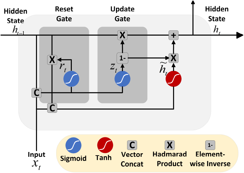
Figure 2.
Single GRU cell architecture. This showcases the primary components including the input layer that receives data, the hidden state carrying information through the network, the reset gate which determines the extent to which previous information is forgotten, and the update gate that decides how much of the current state should be updated with the new proposed state.
GRUs, introduced in [13], are a type of RNN [12] designed to capture long-term dependencies in sequential data while overcoming the short-term memory limitations of traditional RNNs. They have comparable accuracy to other RNN structures like LSTM [14], but offer faster training and prediction due to fewer model parameters [29, 30].
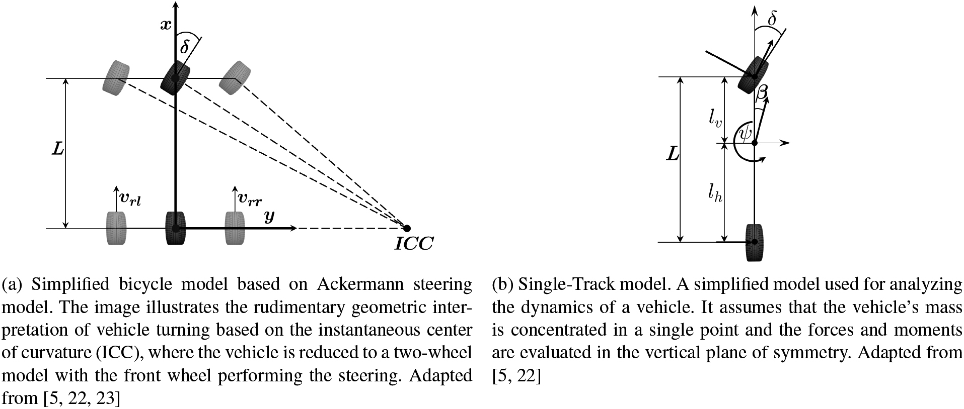
Figure 3.
Comparison between the Ackermann steering model and single-track model.
As Fig. 2 illustrates, the GRU cell is governed by:
(2)
(3)
(4)
(5)
where
Reset Gate
The reset gate (
Update Gate
The update gate (
It’s worth noting that while GRUs inherently transfer information across time steps in a sequence, this mechanism is distinct from the traditional concept of transfer learning, where pre-trained models are adapted for a different but related task [31, 30].
2.3Single track model
The single-track model, a physics-based kinematic model often used as a simplified version of the Ackermann steering model [23, 32], delivers a plausible representation of vehicle behavior without requiring extensive modeling or parameterization [22, 32]. This kinematic model was proposed for lateral accelerations below 0.5 g [32].
The bicycle model, a simplified version of the Ackermann model, as depicted in Fig. 3a, merges the front and rear wheels into single points each. This enables the model to depict lateral vehicle dynamics in a physically plausible manner as illustrated in Fig. 3b [33, 22]. The single-track model’s acceleration around the center of gravity is given by:
(6)
In the single-track model, the vehicle’s mass is assumed to be concentrated at its center of gravity, a common simplification in vehicle dynamics. While this assumption streamlines the model, it may overlook some real-world complexities. However, neural networks, especially CNNs and GRUs, can learn and account for such intricacies. Leveraging the deep learning capabilities highlighted by [34], our hybrid CNN-GRU architecture learns transformations, including those related to the center of mass, enhancing the model’s adaptability and accuracy.
3.State of the art
In this section, we address the topic of VSA estimation as well as CNN-GRU hybrid models. As outlined in the introduction, the majority of VSA estimation methods gravitate towards either a model-based approach, employing a kinematic or dynamic model coupled with an observer, or a black-box model which utilize machine learning models. However, only a few of these approaches exploit a combination of both strategies.
In [35], three FFNN configurations were designed to estimate the VSA. Network A utilized basic vehicle dynamics, while Networks B and C integrated time-delayed signals and feedback for improved accuracy. While A faced challenges with speed variations, B showed adaptability, and C, despite its feedback mechanism, had inconsistent performance. Overall, Network B was the most reliable for estimating the sideslip angle across varying conditions.
The authors of [9] utilized an LSTM RNN in combination with a fully connected layer as output to determine the lateral vehicle velocity which is inherently necessary to calculate the VSA. They collected approx. 88 minutes of simulation data with varying road friction coefficients and applied a 90/10 train-test split. For evaluation they performed a double lane change experiment and reported that their method achieved accurate estimation of the vehicle lateral velocity during low and medium speeds of
In [8] a GRU network was combined with a kinematic model for the estimation of the VSA. The authors collected approx. 16 hours of sensor data, in a real-world vehicle, under three different road conditions and compared their VSA estimation approach with a sensor fusion of GPS and IMU. The authors set a plain GRU network against a hybrid kinematic GRU model for comparison. The former model incorporated inputs such as the steering wheel angle, longitudinal speed, longitudinal and lateral acceleration, yaw rate, and all four wheel speeds for prediction. In contrast, the latter model, aside from using the previously mentioned inputs, also took into account the change in side-slip angle
The authors of [36] proposed a hybrid state estimation approach to estimate the roll angle of a vehicle using a combination of data-based estimators represented by a GRU network and existing physical knowledge. The proposed method was evaluated using real-world driving data and showed improved precision compared to traditional methods such as EKF and UKF. The results showed that the hybrid state estimation approach provided accurate estimates of roll angle compared to traditional methods such as EKF and UKF. The RMSE of roll angle estimation using hybrid state estimation was 0.23
Utilizing the feature extraction capabilities of CNNs and using them as (additional) input for GRU networks has seen an up-rise in recent years as many researches combined the benefits of those two methods creating a CNN-GRU deep learning framework [37, 38, 39, 40, 41].
The combination of CNN and GRU was employed in [40] to learn the dynamic time-series relationship between variable working conditions and clamping point force for the prediction of the clamp force for handling deformable parts. Here a fully connected CNN was utilized for feature extraction and dimensionality reduction of high dimensional data representing the change of force state at the clamping point. The extracted features were utilized as inputs for a GRU network for prediction of the clamping point force under complex time-varying conditions and proved the effectiveness of the CNN-GRU prediction framework.
The research conducted in [37] proposed a two-step hybrid CNN-GRU network to predict short-term electricity consumption in residential buildings. The CNN consisted of two convolutional layers with ReLU activation function and a kernel size of two and a filter of 1
A spatial-temporal feature-selection algorithm was also utilized in [41] to determine relevant inputs for a CNN-GRU for short-term traffic speed prediction. The network structure consisted of the LeNet-5, for the CNN, and a bidirectional GRU, so that the predictions could also incorporate previous inputs in addition to the current input vector for greater accuracy. The findings showed that this hybrid model overcame the constraints of single models, fully utilized the space-time properties of the traffic data, and predicted traffic speeds with high accuracy.
Table 1
Component comparison of state-of-the-art literature with our approach
| [8] | [9] | [35] | [36] | [37] | [40] | [41] | Our | |
| FFNN |
|
| ✓ |
|
|
|
| ✓ |
| LSTM |
| ✓ |
|
|
|
|
|
|
| GRU | ✓ |
|
| ✓ | ✓ | ✓ | ✓ | ✓ |
| VSA estimation | ✓ | ✓ | ✓ |
|
|
|
| ✓ |
| Kinematic model | ✓ |
|
|
|
|
|
| ✓ |
| Snowy conditions | ✓ |
|
|
|
|
|
| ✓ |
| Image features |
|
|
|
|
| ✓ |
| ✓ |
| CNN-GRU hybrid |
|
|
|
| ✓ | ✓ | ✓ | ✓ |
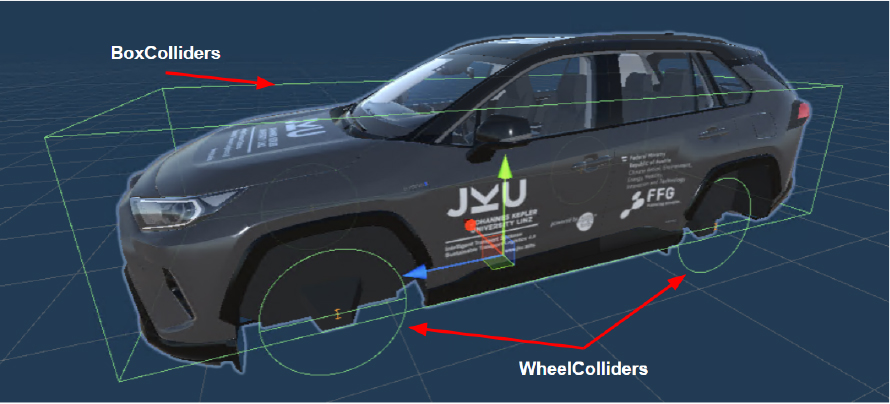
Figure 4.
The car model, as well as the BoxCollider and WheelColliders. The mesh of the wheels are disabled to avoid visual occlusion of the WheelColliders.
Existing research highlights the potential of hybrid GRU models for VSA estimation, but their performance is limited in challenging conditions like snowy environments [8]. The effectiveness of hybrid CNN and GRU models for VSA estimation in adverse conditions remains largely unexplored. Our study addresses this research gap and aims to enhance VSA estimation models by integrating visual cues from camera data thus reducing reliance on error-prone sensors, particularly in challenging snowy road conditions.
To provide a clearer perspective on how our approach stands in comparison to existing literature, we present Table 1 that juxtaposes the key components and features of various state-of-the-art methods with our proposed methodology. This table elucidates the comprehensive nature of our approach, highlighting its distinctiveness and advancements in the field. By examining the table, it becomes evident that our approach amalgamates a diverse set of features and methodologies, setting it apart from the current state-of-the-art literature. This comprehensive integration is pivotal in enhancing the accuracy and robustness of VSA estimation, especially under challenging conditions.
4.Simulation environment and data analysis methods
This section initially presents the simulation environment, which was used to generate the data for this study. Subsequently, we outline the methodology used to explore the relationship between the image-based features and the VSA. Furthermore, this section introduces the proposed model that integrates CNN-based features for accurate VSA estimation.
4.1Experimental setup and simulation environment
We used the Unity3D based 3DCoAutoSim [42] platform to simulate the environment with snowfall, friction, and car tracks on the snow. The test ground setup used in this work is based on [10], which is a snow covered 4-lane dual carriageway circular test track. The friction between the road surface and the wheels is directly achieved by setting the Unity WheelColliders, which will be explained in more detail later. The setting of the test ground is mainly to extract visual data such as car tracks on the snow. For the dataset creation we performed multiple laps, in both directions of the course, and stored the sensor data in separate rosbag files.
The vehicle model in the simulator corresponded to a Toyota Rav4 Hybrid (2020) [43] and closely resembles it in terms of track-width, wheelbase, and mass which is equally distributed over the volume of the vehicle. In order to perform the collision volume of the vehicle, we used a Unity BoxCollider that covered the complete body of the vehicle, being its center of mass selected from the geometric center of the vehicle chassis, as seen in Fig. 4. The four wheels were respectively controlled by four Unity WheelColliders, and their steering occurred in conformity with the Ackermann steering model. The control scripts set of the vehicle relied on [10], which was implemented via the RealisticCarControl V3 [44].
Table 2
The friction parameter settings of the WheelColliders
| Forward friction | Sideways friction | |
| Extremum slip | 0.4 | 0.2 |
| Extremum value | 1 | 1 |
| Asymptote slip | 0.8 | 0.8 |
| Asymptote value | 0.5 | 0.75 |
| Stifness | 1 | 1 |
The parameters of the WheelCollider controlled the friction between the wheels and ground. The default settings of the friction parameters for the experiment are shown in Table 2. We also implemented a 9 degree of freedom Inertial Measurement Unit (IMU), GPS sensor, as well as longitudinal velocity. In addition, we monitored the steering angle of the vehicle as well as the side-slip angle. All these data were either directly received from Unity or calculated from the sensor data. Finally, we used two cameras with a resolution of 640
4.2Analysis of the image data
The foundation of this study is built upon an existing relationship between the data obtained from imaging sensors and the VSA. This approach is motivated by the acknowledged limitations of black-box machine learning models [45].
To develop a reliable model, we performed a comprehensive analysis of this relationship. This involved the collection and processing of image and VSA data from the simulated environment discussed above, conducting rigorous statistical tests to investigate correlations, and scrutinizing the relationship between the variables.
In each timestep
In each timestep, we applied the GoogLeNet CNN [17] and obtained 1024 features for each image. In order to evaluate the relationship between these features and the VSA, we first standardized the features and extracted a de-correlated representation relying on the PCA [19]. We chose a variance-based method (PCA) since it offers a clear and intuitive understanding of the data’s structure. The principal components (lateral dimensions) derived from such methods are orthogonal, ensuring no redundancy, and they capture the directions of maximum variance in the data, making it more readable.
Figure 5.
The proposed method with a batch size of
![The proposed method with a batch size of B, sliding window length of W and a output prediction horizon of P considering only one camera. The proposed approach utilizes various sensor data, including images (img), wheel angular velocities (ωxy), steering angle (δ), longitudinal velocity (vx), longitudinal and lateral acceleration (ax and ay), yaw rate (ψ˙), as well as the derivative of the prediction target (β˙) computed using the kinematic single-track model, as input for time series prediction. The model integrates a CNN [17] for image-based feature extraction and a GRU with two recurrent layers, a hidden dimensionality of 128, and a tanh activation function for capturing temporal dependencies and ensuring effective information transfer across time steps. This amalgamation results in a hybrid kinematic CNN-GRU informed model that leverages exteroceptive data. The dimensionality of the various inputs, as well as the propagated values are displayed within square brackets.](https://content.iospress.com:443/media/ica/2024/31-2/ica-31-2-ica230727/ica-31-ica230727-g005.jpg)
The relationship between the first five principal components and the VSA was assessed using both Pearson’s and Spearman’s rank correlation tests. Pearson’s test was chosen as it effectively measures linear relationships between continuous variables providing insights into any linear correlation between the latent features and
We formulated two null hypotheses for our analysis.
• Null Hypothesis 1, denoted as
• Null Hypothesis 2, denoted as
Both hypotheses tested whether there was a significant relationship between the variables under consideration. If the p-value, the probability of observing the data or more extreme results under the assumption that the null hypothesis is true, was found to be less than the predefined significance level
4.3Model implementation for VSA estimation
Our implemented prediction model consisted of a CNN, specifically GoogLeNet [17], for feature extraction on images, and a GRU, for time series prediction, as visualized in Fig. 5. The choice of GoogLeNet was motivated by its efficiency in feature extraction, computational affordability, and its ability to learn multi-scale features through inception modules [17], metrics that are crucial in various applications, including digital photogrammetry of piping systems [46]. These evaluation criteria align with the comprehensive computational exploration conducted by [47], who also emphasized the importance of methodological choices and feature extraction techniques. The chosen inputs consisted of a sliding window sequence
Furthermore, our research explored both sequence-to-one (S2O) and sequence-to-sequence (S2S) predictions. Specifically, S2O prediction involves processing a sequence of input data to produce a single output, while S2S prediction takes a sequence of input data and predicts a corresponding output sequence, allowing for more dynamic and temporally structured predictions [48]. The examination of different sliding window lengths provides critical insights into the temporal influence on the prediction accuracy of the model. We utilized the last feature map of a CNN [17] to provide exteroceptive information of the environment to the prediction model. We argue that the incorporation of exteroceptive information from image streams provides long term correction data and thus will improve the sequence-to-sequence prediction capabilities. Besides the aforementioned sensor data we utilized the kinematic single-track model to compute the derivative, of the prediction target which is fed to the linear layer via the motion model. For this we transformed the formula Eq. (6) to derive
(7)
We argue that the proposed sensor suit is applicable for the use case due to the fact that (i) all new vehicles manufactured on or after May 1
Table 3
Dataset metrics
| Train | Validate | |
|---|---|---|
| Samples | 64501 | 1418 |
| Minutes | 107.39 | 2.21 |
|
| 0.71 | 3.15 |
|
| 6.24 | 6.03 |
Table 4
3 best validation scores of 3-fold cross validation. Best result in bold
| Hidden dim | N layers | Validation score |
|---|---|---|
| 64 | 2 | 0.0288 |
| 128 | 1 | 0.0266 |
| 128 | 2 | 0.0235 |
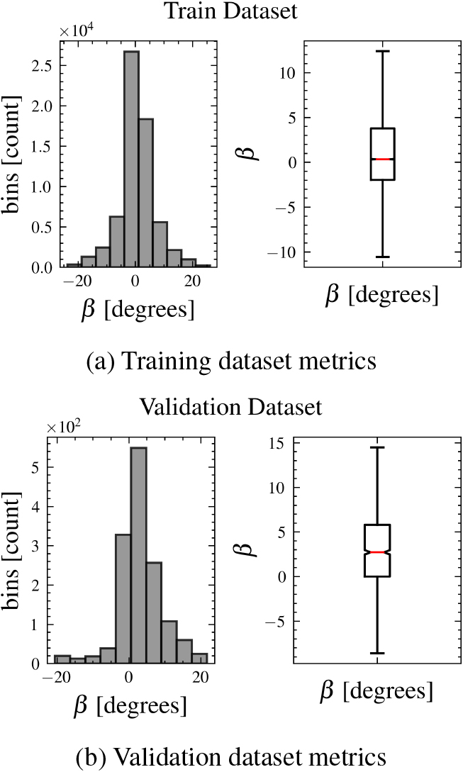
Figure 6.
Dataset metrics.
We implemented the model using PyTorch [53] and Cuda 12.1. To train and test our model we collected a total of 110 min data on snow covered asphalt in the 3DCoAutoSim simulator [54]. Table 3 depicts an overview of the dataset composition. For the initial hyperparameter estimation, we relied on 3-fold cross-validation with 20 epochs, Table 4 visualizes the results and selected parameters. Besides the initially chosen hyperparameters we utilized learning rate scheduling based on ReduceLRonPlateu11 to improve model performance and speed up the training process [55, 56]. Furthermore, to prevent overfitting we implemented early stopping when the validation loss did not decrease for 20% of the overall training epochs, L1-regularization (
Besides the proposed approach shown in Fig. 5, we compared our model in S2O and S2S prediction to the approach implemented in [8]. In all cases we used a separate validation dataset to evaluate our model that was neither used during training nor testing. Since the frequency of the sensors differed, we re-sampled the collected data, in preprocessing, to a frequency of 10 Hz. We then performed outlier removal, by relying on the z-score of 3, which indicates that data points beyond 3 standard deviations from the mean were considered as outliers, and further prepared the dataset in a sliding window approach as depicted in Table 5. Furthermore, we employed a feature scaling technique to normalize the range of the independent variables in the dataset as part of the data preprocessing step. The resulting dataset consisted of 65919 sample points valid for training, testing, and evaluation. Figure 6 visualizes the distribution of the ground truth VSA over the complete dataset.
Table 5
Dataset structure for sequence-to-sequence prediction using a sliding window approach. The table represents input sequences with
|
|
|
|
|
|---|---|---|---|
|
|
|
|
|
|
|
|
|
|
|
|
|
|
|
4.4Model evaluation
In light of the correlation analysis, the highly non-linear feature processing within our proposed CNN pipeline, and the distinct correlation of front and rear camera features with the VSA, we pursued two distinct experimental approaches. These approaches not only included image data but also leveraged other sensor information as previously described in this section.
Approach A utilized both front and rear image data in conjunction with the sensor data. This aimed to assess the combined impact of front and rear cameras and other sensor information on the model’s VSA prediction capabilities.
On the other hand, Approach B focused exclusively on the front image data and the sensor information, intentionally omitting the rear image data. Despite using the same dataset as Approach A, Approach B truncated the rear camera information. The rationale behind this strategy was to test the relevance and impact of the rear camera data as suggested by the correlation analysis.
4.4.1Sequence-to-one prediction
To evaluate the precision of both models in the S2O prediction paradigm, we employed the sMAPE, as elaborated at the end of this Section. For the performance of our proposed hybrid CNN-GRU model on the task of S2O prediction we set during training the hyperparameter
4.4.2Sequence-to-sequence prediction
Given the interdependent nature of the VSA data, which dynamically evolves based on past, present, and future states, the S2S prediction paradigm is integral to our models, designed to capture and interpret the complex temporal dependencies that exist among different states in a sequence, thereby producing accurate estimations of future vehicle side-slip angles.
To evaluate the effectiveness of our S2S models, we conducted a series of comparative analyses using different prediction horizons. We employed the sSMAPE as our performance metric, providing a robust measure of the prediction accuracy of our models across various time horizons
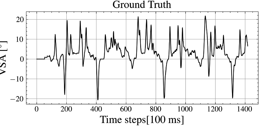
Figure 7.
Ground truth VSA of the evaluation dataset.
The outcomes yielded by our two experimental strategies in relation to the two distinct prediction paradigms, S2O and S2S, are delineated in Sections 5.2 and 5.3, respectively. To further fine-tune our models, we trained them using an array of hyperparameter combinations, these encompassed various sliding window input sizes
Finally, we evaluated the model performance using the sMAPE, sequence wise sMAPE (sSMAPE) as well as the averaged sSMAPE (
sMAPE
For evaluating the models’ accuracy we relied on sMAPE, the most commonly used metric to determine the accuracy of time sequence predictions [57]. Further, the sMAPE metric is especially suited for forecasting problems, as it provides a symmetric, scale-independent error measure, which is particularly useful when dealing with datasets that may contain zeros, as seen in Eq. (8) [58].
(8)
being
Table 6
Statistical investigation of the relation of the PCA-based processed CNN features of the front and rear camera to
| Front | Rear | |||||||
|---|---|---|---|---|---|---|---|---|
| Pearson’s corr. | Spearman’s rank corr. | Pearson’s corr. | Spearman’s rank corr. | |||||
| PCA dimension | Estimate | p-value | Estimate | p-value | Estimate | p-value | Estimate | p-value |
| 1 | 1e-4 | 0.0006 | 0.0615 | 1e-4 | 0.0686 | 1e-4 | ||
| 2 | 0.1951 | 1e-4 | 0.1800 | 1e-4 | 0.0816 | 1e-4 | 0.1268 | 1e-4 |
| 3 | 1e-4 | 1e-4 | 1e-4 | 1e-4 | ||||
| 4 | 0.0876 | 1e-4 | 0.1119 | 1e-4 | 0.0013 | 0.0037 | 0.7144 | |
| 5 | 0.2232 | 1e-4 | 0.2095 | 1e-4 | 1e-4 | 0.0048 | ||
Sequence wise sMAPE
In our computation, we applied Eq. (8) to the predictions generated by our sequence-to-one/sequence model. Given that our model produced a set of sequences as its prediction output, the calculation was done on a per-sequence basis over all time steps and subsequently divided by the total number of time steps, yielding the sMAPE per sequence sSMAPE (sequence wise sMAPE) as described in Eq. (4.4):
(9)
In this equation,
Averaged sSMAPE
To provide a comprehensive overview of the performance of the models, we averaged the error metrics across all prediction sequences. This mean error, as seen in Eq. (10), represented the overall performance of the models across different prediction horizons and offered a summary measure of their accuracy.
(10)
where
5.Results
This section describes the results of the relationship analysis of CNN image features and the VSA
5.1Correlation analysis
Table 6 reports the detailed findings of the correlation analysis described in 4.2, summarizing the estimated correlation values and their associated p-values for both Pearson’s and Spearman’s rank correlation methods. Each row represents one of the principal components from the PCA-based processed CNN features. Each column shows the estimate and p-value of the respective correlation method for both the front and rear cameras.
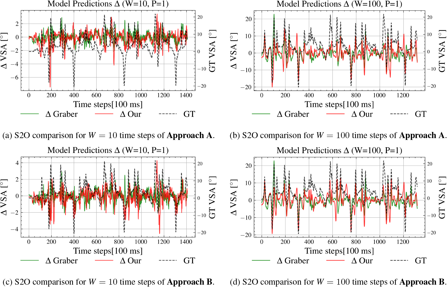
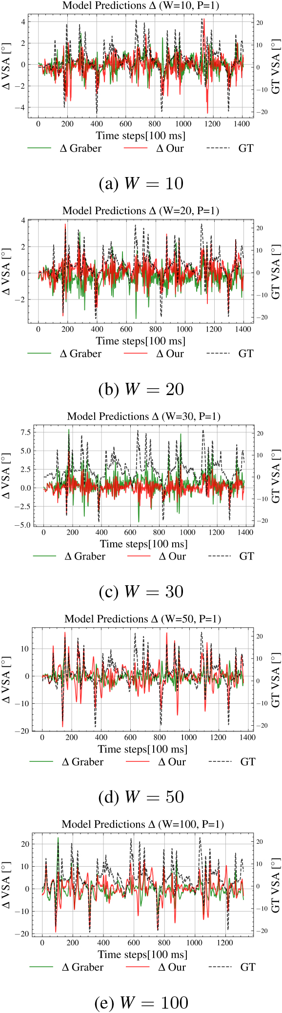
Figure 8.
Comparative differential plots of S2O predictions from Approach A (middle) and Approach B (bottom), showing deviation from ground truth. Different input window lengths of
5.2Sequence-to-one prediction model evaluation
Figure 8 showcases the effectiveness of our hybrid CNN-GRU model in executing the S2O prediction task. It presents comparative differential plots for both Approach A and Approach B under different sliding window lengths of
Table 7
sSMAPE compared to ground truth for
| Window size | Approach A | Approach B | [8] |
|---|---|---|---|
| 10 | 0.410 | 0.387 | 0.366 |
| 20 | 0.373 | 0.340 | 0.335 |
| 30 | 0.376 | 0.318 | 0.454 |
| 50 | 0.741 | 0.778 | 0.478 |
| 100 | 0.783 | 0.827 | 0.754 |
Figure 9.
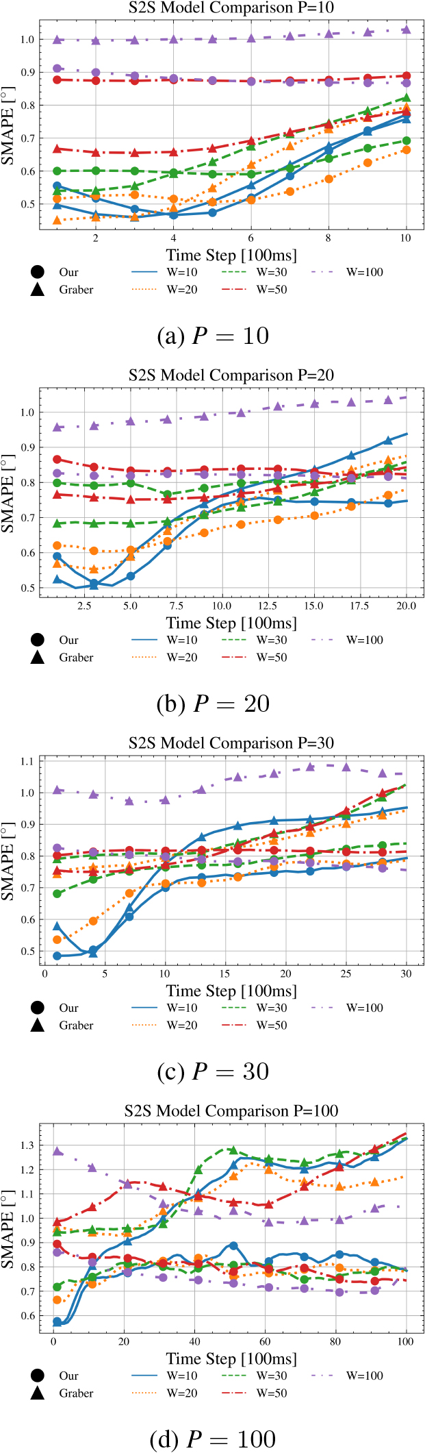
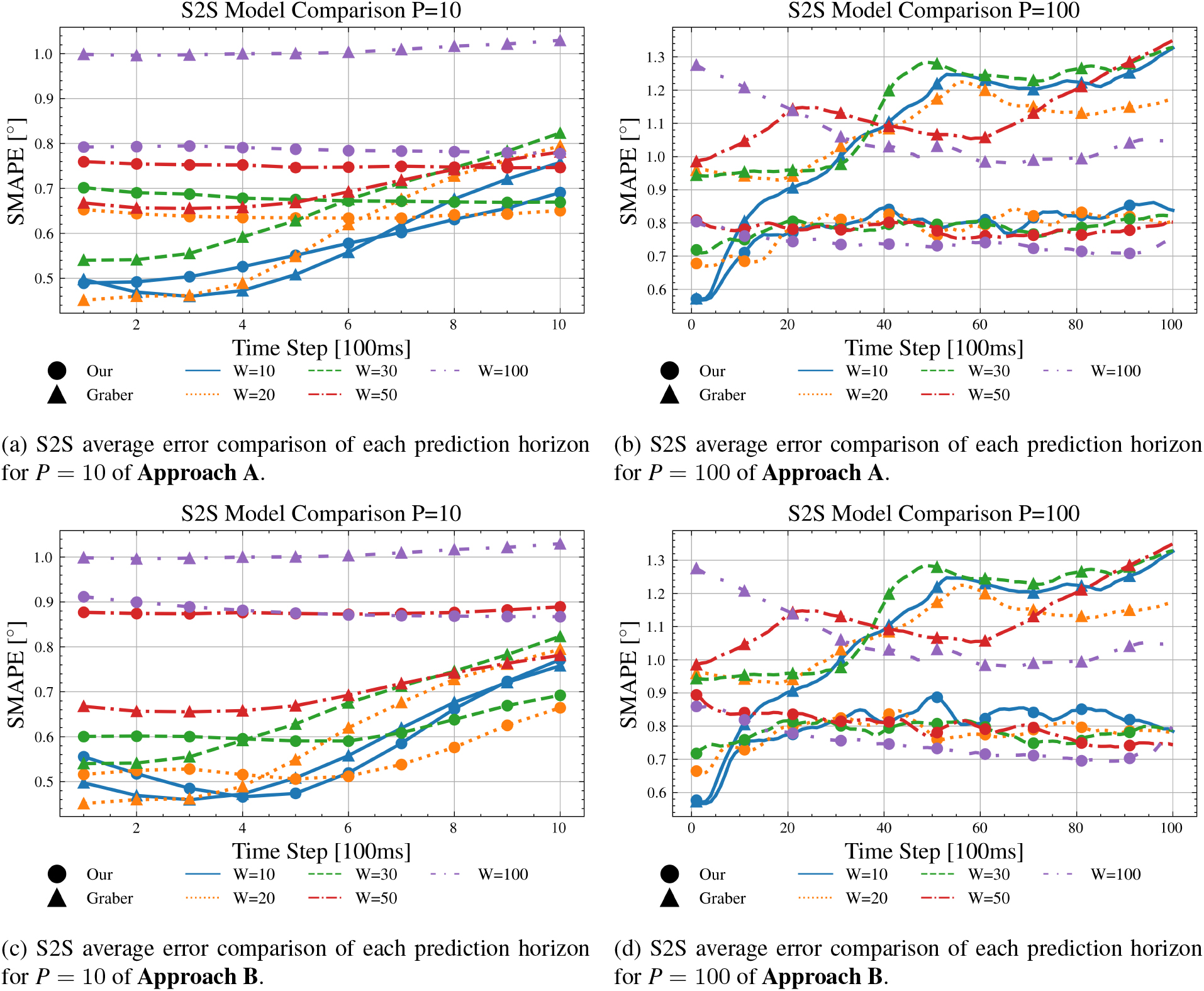
S2S sSMAPE comparison for each individual prediction horizon sequence.
In Fig. 8a and c we can see that, compared to the ground truth and the approach of [8], our models generated similar accurate results, except for cases when the target value is close to the min/max values of the training data, e.g. as seen at
5.3Sequence-to-sequence prediction model evaluation
Table 8
Comparison of Average Errors (
| Prediction horizon | Window size | Approach A | Approach B | [8] |
|---|---|---|---|---|
|
| 10 | 0.572 | 0.576 | 0.574 |
| 20 | 0.641 | 0.551 | 0.599 | |
| 30 | 0.679 | 0.6819 | 0.660 | |
| 50 | 0.750 | 0.877 | 0.700 | |
| 100 | 0.787 | 0.880 | 1.007 | |
|
| 10 | 0.645 | 0.673 | 0.737 |
| 20 | 0.672 | 0.674 | 0.719 | |
| 30 | 0.731 | 0.800 | 0.739 | |
| 50 | 0.807 | 0.835 | 0.780 | |
| 100 | 0.794 | 0.820 | 0.999 | |
|
| 10 | 0.685 | 0.693 | 0.805 |
| 20 | 0.721 | 0.717 | 0.835 | |
| 30 | 0.757 | 0.778 | 0.863 | |
| 50 | 0.827 | 0.815 | 0.845 | |
| 100 | 0.756 | 0.788 | 1.031 | |
|
| 10 | 0.788 | 0.802 | 1.084 |
| 20 | 0.786 | 0.782 | 1.085 | |
| 30 | 0.785 | 0.783 | 1.149 | |
| 50 | 0.780 | 0.799 | 1.131 | |
| 100 | 0.783 | 0.748 | 1.064 |
Figure 9 presents the outcomes of applying the S2S prediction paradigm, illustrating the sSMAPE metric at each prediction horizon. For a more granular perspective see Table 8, as it displays the mean sSMAPE
The comparison of S2S averaged sMAPE for each individual prediction sequence for different horizons
The comparison of the S2S prediction paradigms is demonstrated through Fig. 9, which illustrates the sSMAPE for each prediction horizon. The results for
When comparing Approach A with Approach B, results for the first prediction step show Approach A surpassing Approach B only in 2 out of 5 instances when
For the last prediction step, the dynamics shift somewhat. Approach A surpasses Approach B in 4 out of 5 cases when
Another point of comparison is the fluctuation of the sSMAPE over time. As depicted in Fig. 9a and c, our models generally exhibit an initial decrease in the sSMAPE which eventually increases after reaching a minimum. In contrast, the model of [8] holds a stable sSMAPE for the early time steps, followed by an increase. This observation suggests that both our models surpass the model of [8] in long-term predictions, with the exact intersection point varying based on the window size
Finally, the models were compared based on their average sSMAPE (
6.Discussion
6.1Correlation analysis
The results of the correlation analysis presented in Table 6 demonstrate several key insights regarding the relationship between PCA-based processed CNN features of the front and rear camera to
High correlations are observed in the second, third, and fifth latent dimensions with
These results are echoed by the Spearman’s rank correlation, suggesting that these statistical relationships are robust. The third latent dimension, in particular, shows a negative correlation, implying an inverse relationship with the VSA in this dimension. The first and fourth latent dimensions also display correlations significant at
The correlations for the rear camera present a different narrative, being notably lower across all latent dimensions compared to the front camera. Nevertheless, most latent dimensions still display statistical significance at
6.2Sequence-to-one prediction
Based on the results of the S2O prediction paradigm we recognize the need for a more in-depth exploration of our model’s capacity. We recognize that (i) additional data augmentation or an expanded training dataset may be necessary for superior data extrapolation. This realization emerged as we compared our approach to that of [8]. On the other hand, (ii) the divergence could also be rooted in the different methodologies for feature extraction from sensor data between our model and [8]’s. Furthermore, (iii) our model extends beyond the approach of [8] by incorporating exteroceptive sensor data, specifically image streams from vehicle cameras processed via CNN. Consequently, our CNN-GRU model captures a different spectrum of information for predicting the extremes of the VSA compared to a standalone GRU. This divergence may contribute to reduced accuracy near the extreme values of the training data. As we continue to refine our model, adjustments to the CNN and the inclusion of supplementary data sources are avenues we plan to explore for improving accuracy.
6.3Sequence-to-sequence prediction
Approach A seems to be slightly more beneficial, especially for window sizes
It is worth noting that Approach A surpassed Approach B in 13 out of 25 cases. This indicates that notwithstanding the diminished correlation of the rear camera features with the side-slip angle, these features nonetheless deliver consequential information that augments the prediction accuracy of our model. The origin of this discrepancy may be rooted in various elements. First and foremost, the nexus between the rear camera features and the side-slip angle could be non-linear and intricate, reducing its detectability by conventional correlation measures but can still be deciphered by state-of-the-art prediction models such as deep neural networks. The sophisticated architecture of such models enables them to extract latent, non-linear patterns in data, thereby enhancing prediction performance even in the absence of an evident linear relationship. Secondly, an overlooked aspect in the correlation analysis is the potential synergistic effect among different data types. In this scenario, the interaction of rear camera features with other pieces of information, such as front camera features or steering angle, could substantially enrich the predictive capacity of the model. This collective effect is not discernible by examining individual correlation coefficients, which provide a somewhat simplistic view of the relationship between individual variables and the target. Lastly, it is plausible that the rear camera features serve as particularly vital information in specific circumstances, for instance, when the vehicle is reversing or during a sharp turn. Such contextual utility of rear camera features contributes to a comprehensive, more accurate prediction across a variety of situations. Taken together, these observations highlight the importance of including diverse types of data in complex prediction tasks, even those with seemingly low correlation to the target variable. It underlines the multifaceted nature of data utility in model performance and cautions against over-reliance on individual correlation measures when making decisions about feature inclusion. The analysis thus suggests the potential benefit of leveraging machine learning models capable of capturing both linear and non-linear relationships and interactions among features.
Compared to the baseline model of [8] both of our models outperformed it for longer prediction horizons (
7.Conclusion and future research
In this work we presumed that the incorporation of CNN features from the cameras of a car can besides the normally utilized kinematic and dynamic parameters improve the estimation of the side-slip angle. Our statistical analysis results revealed a significant relationship between the second, third, and fifth latent dimensions of the front camera and the side-slip angle (denoted as
Contrary to the correlation analysis results, our empirical investigation, relying on our hybrid CNN-GRU, illuminated that exploiting all available features (Approach A) often led to superior side-slip angle predictions relative to utilizing all features excluding the rear camera features (Approach B).
Our investigation concentrated on three principal areas: correlation analysis, sequence-to-one prediction, and sequence-to-sequence prediction. In Section 4.2 we explored the relationships between latent variables inherent to the front and rear image features and the VSA
The insights gained from these results contribute to a wider understanding as they do not only highlight the efficacy of our proposed models but also underscore potential limitations, particularly in utilizing the S2S prediction paradigm in VSA estimation. The real-world applicability of our model is evident in its potential to improve vehicle control in adverse conditions like snow. Its strength in longer prediction horizons makes it valuable for autonomous driving systems, where precise side-slip angle estimation is crucial for safety. The model’s ability to integrate diverse sensor data also adds contextual adaptability, useful in specific driving scenarios such as reversing or sharp turns.
Future research is needed to confirm these results and should consider integrating attention mechanisms and encoder-decoder structures into the model. Attention mechanisms could enhance feature relevance at each time step, potentially improving prediction accuracy. Moreover, encoder-decoder or autoencoder structures might enhance performance for larger input window sizes and prediction horizons, as they are adept at capturing temporal dependencies in sequence-to-sequence prediction tasks. These adjustments could offer a promising avenue for model performance improvement in side-slip angle prediction. In addition to the aforementioned avenues for future research, it may be beneficial to explore different CNN architectures to optimize VSA estimation. This could include direct estimation as well as the use of temporally contiguous gray-scale images. Ablation studies could help to isolate the effects of each architectural component and input modality and separate projection layers for each input could offer more flexibility in learning the weights and biases for each input. Moreover, investigating the use of sensors to dynamically determine the most suitable approach based on conditional probabilities and safety conditions could provide a more adaptive and robust system for VSA estimation on real systems. Finally, considering different hybrid models tailored to specific input states might optimize a first step towards real-time performance of the hybrid model. As an alternative to the current use of PCA for dimensionality reduction, future research could consider other dimensionality reduction methods such as [59] for discovering the most effective feature spaces and optimizing the number of features. This could provide a more robust and accurate approach for VSA estimation.
Notes
1 Used to reduce learning rate when a metric has stopped improving https://pytorch.org/docs/stable/generated/torch.optim.lr_scheduler.ReduceLROnPlateau.html.
2 We had to implement a minor modification on the output regression head so that the model could also be used for S2S prediction.
References
[1] | Robert Bosch GmbH [homepage on the Internet]. Vehicle dynamics control 2.0. (2022) [updated 2022; cited 2022 Dec 16]. Available from: https://www.bosch-mobility.com/en/solutions/driving-safety/vehicle-dynamics-control/. |
[2] | Chindamo D, Lenzo B, Gadola M. On the vehicle sideslip angle estimation: A literature review of methods, models, and innovations. Applied Sciences (Switzerland). (2018) ; 8: (3). |
[3] | Liu J, Wang Z, Zhang L, Walker P. Sideslip angle estimation of ground vehicles: A comparative study. IET Control Theory and Applications. (2020) ; 14: (20): 3490-505. |
[4] | Essa MG, Elias CM, Shehata OM. Comprehensive Performance Assessment of Various NN-based Side-Slip Angle Estimators (ANN-SSE). In: 2021 IEEE 93rd Vehicular Technology Conference (VTC2021-Spring). (2021) . pp. 1-6. |
[5] | Rajamani R. Lateral vehicle dynamics. In: Vehicle Dynamics and Control. Springer; (2012) . pp. 15-46, 201-3. |
[6] | Biase FD, Lenzo B, Timpone F. Vehicle sideslip angle estimation for a heavy-duty vehicle via extended kalman filter using a rational tyre model. IEEE Access. (2020) ; 8: : 142120-30. |
[7] | Kim D, Kim G, Choi S, Huh K. An integrated deep ensemble-unscented Kalman filter for sideslip angle estimation with sensor filtering network. IEEE Access. (2021) ; 9: : 149681-9. |
[8] | Graber T, Lupberger S, Unterreiner M, Schramm D. A hybrid approach to side-slip angle estimation with recurrent neural networks and kinematic vehicle models. IEEE Transactions on Intelligent Vehicles. (2019) ; 4: (1): 39-47. |
[9] | Kong D, Wen W, Zhao R, Lv Z, Liu K, Liu Y, Gao Z. Vehicle lateral velocity estimation based on long short-term memory network. World Electric Vehicle Journal. (2022) ; 13: (1). |
[10] | Liu Y, Morales-Alvarez W, Novotny G, Olaverri-Monreal C. Study of ROS-Based Autonomous Vehicles in Snow-Covered Roads by Means of Behavioral Cloning Using 3DCoAutoSim. Lecture Notes in Networks and Systems. (2022) ; 470 LNNS: 211-21. |
[11] | Bebis G, Georgiopoulos M. Feed-forward neural networks. IEEE Potentials. (1994) ; 13: (4): 27-31. |
[12] | Rumelhart DE, McClelland JL. Learning Internal Representations by Error Propagation. In: Learning Internal Representations by Error Propagation. MIT Press; (1987) . pp. 318-62. |
[13] | Cho K, van Merriënboer B, Bahdanau D, Bengio Y. On the properties of neural machine translation: Encoder-decoder approaches. In: Proceedings of SSST 2014 – 8th Workshop on Syntax, Semantics and Structure in Statistical Translation. Association for Computational Linguistics (ACL); (2014) . pp. 103-11. |
[14] | Hochreiter S, Schmidhuber J. Long short-term memory. Neural Computation. (1997) ; 9: (8): 1735-80. |
[15] | Carranza-García M, Galán-Sales FJ, Luna-Romera JM, Riquelme JC. Object detection using depth completion and camera-LiDAR fusion for autonomous driving. Integrated Computer-Aided Engineering. (2022) ; 29: (3): 241-58. |
[16] | Hüpen P, Kumar H, Shymanskaya A, Swaminathan R, Habel U. Impulsivity classification using EEG power and explainable machine learning. International Journal of Neural Systems. (2023) ; 33: (02): 2350006. PMID: 36632032. Available from: doi: 10.1142/S0129065723500065. |
[17] | Szegedy C, Liu W, Jia Y, Sermanet P, Reed S, Anguelov D, Erhan D, Vanhoucke V, Rabinovich A. Going deeper with convolutions. In: Proceedings of the IEEE Conference on Computer Vision and Pattern Recognition. (2015) . pp. 1-9. |
[18] | Pett MA. Nonparametric statistics for health care research: Statistics for small samples and unusual distributions. Sage Publications; (2015) . |
[19] | Bishop CM, Nasrabadi NM. Pattern recognition and machine learning. vol. 4. Springer; (2006) . |
[20] | Albawi S, Mohammed TA, Al-Zawi S. Understanding of a convolutional neural network. In: Proceedings of 2017 International Conference on Engineering and Technology, ICET 2017. vol. 2018-Janua. Institute of Electrical and Electronics Engineers Inc.; (2018) . pp. 1-6. |
[21] | Alom MZ,Taha TM, Yakopcic C, Westberg S, Sidike P, Nasrin MS, Hasan M, Van Essen BC, Awwal AAS, Asari VK. A state-of-the-art survey on deep learning theory and architectures. Electronics 2019, Vol 8, Page 292. (2019) 3; 8: (3): 292. Available from: https://www.mdpi.com/2079-9292/8/3/292/htmhttps://www.mdpi.com/2079-9292/8/3/292. |
[22] | Dieter Schramm Manfred Hiller RBa. Vehicle Dynamics: Modeling and Simulation. 2nd ed. Springer; (2018) . |
[23] | Jazar RN. Vehicle dynamics: theory and application. Springer; (2017) . |
[24] | Farah S, David AW, Humaira N, Aneela Z, Steffen E. Short-term multi-hour ahead country-wide wind power prediction for Germany using gated recurrent unit deep learning. Renewable and Sustainable Energy Reviews. (2022) 10; 167: : 112700. |
[25] | Sachin S, Tripathi A, Mahajan N, Aggarwal S, Nagrath P. Sentiment analysis using gated recurrent neural networks. SN Computer Science. (2020) Mar; 1: (2): 74. Available from: doi: 10.1007/s42979-020-0076-y. |
[26] | Wazrah AA, Alhumoud S. Sentiment analysis using stacked gated recurrent unit for arabic tweets. IEEE Access. (2021) ; 9: : 137176-87. Available from: https://www.kaggle.com/monsterspy/conv-lstm-sentiment-analysis-. |
[27] | Wöber W, Curto M, Tibihika P, Meulenbroek P, Alemayehu E, Mehnen L, Meimberg H, Sykacek P. Identifying geographically differentiated features of Ethopian Nile tilapia (Oreochromis niloticus) morphology with machine learning. PLOS ONE. (2021) ; 16: (4): 1-30. Available from: doi: 10.1371/journal.pone.0249593. |
[28] | Yin W, Kann K, Yu M, Schütze H. Comparative Study of CNN and RNN for Natural Language Processing. arXiv. (2017) . Available from: http://arxiv.org/abs/1702.01923. |
[29] | Shewalkar A, Nyavanandi D, Ludwig SA. Performance evaluation of deep neural networks applied to speech recognition: Rnn, LSTM and GRU. Journal of Artificial Intelligence and Soft Computing Research. (2019) 10; 9: (4): 235-45. Available from: https://www.infona.pl//resource/bwmeta1.element.baztech-0106e25d-92b6-4c93-8317-367a9f574578. |
[30] | Chung J, Gülçehre Ç, Cho K, Bengio Y. Empirical Evaluation of Gated Recurrent Neural Networks on Sequence Modeling. CoRR. (2014) ; abs/1412.3555. Available from: http://arxiv.org/abs/1412.3555. |
[31] | Farahani A, Pourshojae B, Rasheed K, Arabnia HR. A Concise Review of Transfer Learning. CoRR. (2021) ; abs/2104.02144. Available from: https://arxiv.org/abs/2104.02144. |
[32] | Polack P, Altché F, d’Andréa Novel B, de La Fortelle A. The kinematic bicycle model: A consistent model for planning feasible trajectories for autonomous vehicles? In: 2017 IEEE Intelligent Vehicles Symposium (IV). (2017) . pp. 812-8. |
[33] | Corke P. Robotics, Vision and Control. vol. 118 of Springer Tracts in Advanced Robotics. Cham: Springer Cham; (2017) . Available from: http://link.springer.com/10.1007/978-3-319-54413-7. |
[34] | LeCun Y, Bengio Y, Hinton G. Deep learning. Nature. (2015) ; 521: (7553): 436-44. |
[35] | Melzi S, Resta F, Sabbioni E. Vehicle sideslip angle estimation through neural networks: application to numerical data. In: Engineering Systems Design and Analysis. vol. 42495; (2006) . pp. 167-72. |
[36] | Sieberg PM, Blume S, Harnack N, Maas N, Schramm D. Hybrid State Estimation Combining Artificial Neural Network and Physical Model. 2019 IEEE Intelligent Transportation Systems Conference (ITSC). (2019) . pp. 894-9. |
[37] | Sajjad M, Khan ZA, Ullah A, Hussain T, Ullah W, Lee MY, Baik SW. A novel CNN-GRU-based hybrid approach for short-term residential load forecasting.IEEE Access. (2020) ; 8: : 143759-68. |
[38] | Hasannezhad M, Ouyang Z, Zhu WP, Champagne B. An Integrated CNN-GRU Framework for Complex Ratio Mask Estimation in Speech Enhancement. 2020 Asia-Pacific Signal and Information Processing Association Annual Summit and Conference, APSIPA ASC 2020 – Proceedings. (2020) . pp. 764-8. |
[39] | Yu J, Zhang X, Xu L, Dong J, Zhangzhong L. A hybrid CNN-GRU model for predicting soil moisture in maize root zone. Agricultural Water Management. (2021) ; 245: (June 2020): 106649. Available from: doi: 10.1016/j.agwat.2020.106649. |
[40] | Li E, Zhou J, Yang C, Wang M, Li Z, Zhang H, Jiang T. CNN-GRU network-based force prediction approach for variable working condition milling clamping points of deformable parts. International Journal of Advanced Manufacturing Technology. (2022) ; 119: (11-12): 7843-63. Available from: doi: 10.1007/s00170-021-08520-2. |
[41] | Ma C, Zhao Y, Dai G, Xu X, Wong SC. A Novel STFSA-CNN-GRU Hybrid Model for Short-Term Traffic Speed Prediction. IEEE Transactions on Intelligent Transportation Systems. (2022) . |
[42] | Hussein A, Diaz-Alvarez A, Armingol JM, Olaverri-Monreal C. 3DCoAutoSim: Simulator for Cooperative ADAS and Automated Vehicles. IEEE Conference on Intelligent Transportation Systems, Proceedings, ITSC. 2018 12; 2018-November. pp. 3014-9. |
[43] | Certad N, Morales-Alvarez W, Novotny G, Olaverri-Monreal C. JKU-ITS automobile for research on autonomous vehicles. In: International Conference on Computer Aided Systems Theory. Springer; (2022) . pp. 329-36. |
[44] | BoneCracker Games [homepage on the Internet]. Realistic Car Controller | Physics | Unity Asset Store. Unity Technologies; 2023. (2023) [updated 2023 Jul 23; cited 2023 Jul 30]. Available from: https://assetstore.unity.com/packages/tools/physics/realistic-car-controller-16296. |
[45] | Lapuschkin S, Wäldchen S, Binder A, Montavon G, Samek W, Müller KR. Unmasking Clever Hans predictors and assessing what machines really learn. Nature Communications. (2019) ; 10: (1): 1096. |
[46] | Tian Y, Ding C, Lin YF, Ma S, Li L. Automatic feature type selection in digital photogrammetry of piping. Computer-Aided Civil and Infrastructure Engineering. (2022) ; 37: (10): 1335-48. Available from: https://onlinelibrary.wiley.com/doi/abs/10.1111/mice.12840. |
[47] | Graña M, Silva M. Impact of machine learning pipeline choices in autism prediction from functional connectivity data. International Journal of Neural Systems. (2021) ; 31: (04): 2150009. PMID: 33472548. Available from: doi: 10.1142/S012906572150009X. |
[48] | Brownlee J. Deep learning for time series forecasting: predict the future with MLPs, CNNs and LSTMs in Python. Machine Learning Mastery; (2018) . |
[49] | Huntley, Mike. Federal motor vehicle safety standard no. 111, Rear Visibility; (2019) . Available from: https://www.federalregister.gov/documents/2019/10/10/2019-22036/federal-motor-vehicle-safety-standard-no-111-rear-visibility. |
[50] | Statista Inc [homepage on the Internet]. Worldwide shipments of cameras for cars in between 2014 and 2020 (in million units). 2022. (2023) [updated 2023 Jan 6; cited 2023 Jul 15]. Available from: https://www.statista.com/statistics/262015/worldwide-shipments-of-cameras-for-cars/. |
[51] | Campbell S, O’Mahony N, Krpalcova L, Riordan D, Walsh J, Murphy A, Ryan C. Sensor Technology in Autonomous Vehicles: A review. In: 2018 29th Irish Signals and Systems Conference (ISSC). (2018) . pp. 1-4. |
[52] | Varghese JZ, Boone RG, others. Overview of autonomous vehicle sensors and systems. In: International Conference on Operations Excellence and Service Engineering. sn; (2015) . pp. 178-91. |
[53] | Paszke A, Gross S, Massa F, Lerer A, Bradbury J, Chanan G, Killeen T, Lin Z, Gimelshein N, Antiga L, Desmaison A, Köpf A, Yang E, DeVito Z, Raison M, Tejani A, Chilamkurthy S, Steiner B, Fang L, Bai J, Chintala S. PyTorch: An Imperative Style, High-Performance Deep Learning Library. Advances in Neural Information Processing Systems. (2019) 12; 32. Available from: https://arxiv.org/abs/1912.01703v1. |
[54] | Olaverri-Monreal C, Errea-Moreno J, Díaz-Álvarez A, Biurrun-Quel C, Serrano-Arriezu L, Kuba M. Connection of the SUMO microscopic traffic simulator and the unity 3D game engine to evaluate V2X communication-based systems. Sensors. (2018) ; 18: (12): 4399. |
[55] | Konar J, Khandelwal P, Tripathi R. Comparison of Various Learning Rate Scheduling Techniques on Convolutional Neural Network. 2020 IEEE International Students’ Conference on Electrical, Electronics and Computer Science, SCEECS 2020. 2020 2. |
[56] | Fernández-Rodríguez JD, Palomo EJ, Ortiz-de Lazcano-Lobato JM, Ramos-Jiménez G, López-Rubio E. Dynamic learning rates for continual unsupervised learning. Integrated Computer-Aided Engineering. (2023) ; 30: : 257-73. 3. Available from: doi: 10.3233/ICA-230701. |
[57] | Martínez F, Charte F, Frías MP, Martínez-Rodríguez AM. Strategies for time series forecasting with generalized regression neural networks. Neurocomputing. (2022) 6; 491: : 509-21. |
[58] | PyTorch Foundation [homepage on the Internet]. Symmetric Mean Absolute Percentage Error. Lightning-AI; 2023. (2023) [updated 2023; cited 2023 Jul 15]. Available from: https://torchmetrics.readthedocs.io/en/stable/regression/symmetric_mean_absolute_percentage_error.html. |
[59] | Rafiei MH, Adeli H. A new neural dynamic classification algorithm. IEEE Transactions on Neural Networks and Learning Systems. (2017) ; 28: (12): 3074-83. |
Appendices
Appendix A. S2O Differential Plots
Figure 10.
S2O differential plots of Approach A for window sizes
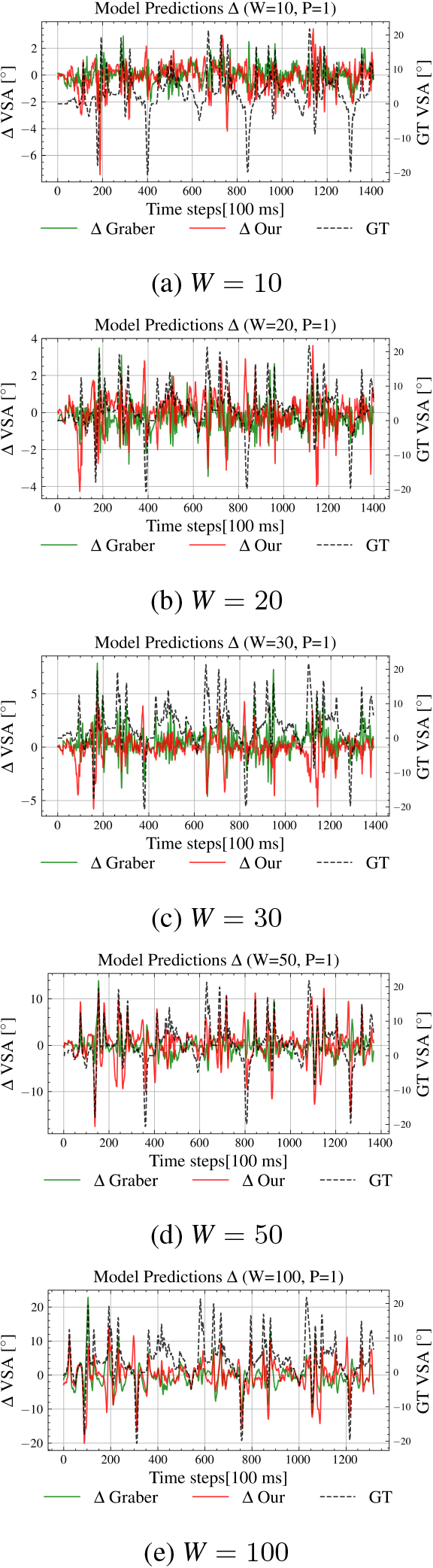
Figure 11.
S2O differential plots of Approach B for window sizes
Appendix B. S2S Average Error Comparison
Figure 12.
S2S averaged sMAPE comparison for Approach A for different horizons
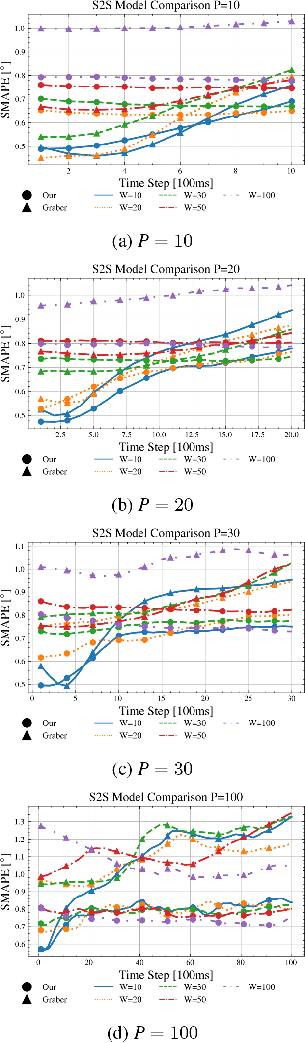
Figure 13.
S2S averaged sMAPE comparison for Approach B for different horizons