Solution of Inverse Problem for Diffusion Equation with Fractional Derivatives Using Metaheuristic Optimization Algorithm

1Introduction

Nowadays, when all kinds of computational and simulation methods are becoming more and more important and the processing power of computers is increasing, it is worth developing and looking for new applications of this type of tools. In practice, there are many classical numerical methods that are successfully used, developed and adapted to current problems. On the other hand, in recent years, scientists have been developing artificial intelligence methods, which include metaheuristic optimization algorithms. In this paper, we focused on combining a classical numerical method for solving a differential equation and selected heuristic algorithms for solving the inverse problem.

In the scientific literature, many works on the use of fractional derivatives to model many processes occurring in physics and engineering can be found (Bhangale et al., 2023; Brociek et al., 2017, 2019; Sowa et al., 2023; Bohaienko and Gladky, 2023; Koleva et al., 2021). In particular, derivatives of this type are used to model anomalous diffusion. As an example, heat flow in porous materials can be mentioned (Brociek et al., 2017, 2019). In article (Brociek et al., 2019), the authors model the phenomenon of heat flow in a porous medium. For this purpose, several mathematical models were used, including those based on fractional derivatives. The results from numerical experiments were compared with measurement data. Models that used fractional derivatives proved to be more accurate than the model with integer-order derivatives. Sowa et al. (2023) used fractional calculus and presented a voltage regulator extended model. The approach presented in the paper for modelling a voltage regulator has been verified with measurement data, and the non-integer order Caputo derivative proved to be an effective tool. Another application of fractional derivatives in mathematical modelling can be found in the paper (Bohaienko and Gladky, 2023), where a model for predicting the dynamics of moisture transport in fractal-structured soils was presented. The model incorporates the Caputo derivative. The numerical solution was obtained using the Crank-Nicholson finite-difference scheme. More examples and trends in the application of fractional calculus in various scientific fields are available in the publications (Hristov, 2023b; Obembe et al., 2017; Ionescu et al., 2017). Publications related to numerical methods in the field of fractional calculus are also worth mentioning (Ciesielski and Grodzki, 2024; Hou et al., 2023; Arul et al., 2022; Hristov, 2023a; Podlubny, 1999; Stanisławski, 2022).

In many engineering problems, there is a need to solve what’s known as an ‘inverse problem’. In simple terms, these issues involve identifying the input parameters of a model (e.g. boundary conditions or material parameters) based on observations (outputs) of the model. Typically, these problems are challenging because they are ill-posed (Aster et al., 2013c; Kaipio and Somersalo, 2005). Examples of inverse problems in various applications are included in the articles (Montazeri et al., 2022; Brociek et al., 2024; Ashurov et al., 2023; Wang et al., 2023; Ibraheem and Hussein, 2023; Brociek et al., 2023; Magacho et al., 2023). For example, the article (Brociek et al., 2024) focuses on an inverse problem concerning the identification of the aerothermal heating of a reusable launch vehicle based on temperature measurements taken in the thermal protection system (TPS) of this vehicle. The mathematical model of the TPS presented in the paper takes into account the dependence on temperature of the material parameters, as well as the thermal resistances occurring in the contact zones of the layers. To solve the inverse problem, the Levenberg-Marquardt method was applied.

One approach to solving inverse problems is to create a fitness function (or loss function, error function), and then optimize it to find the identified parameters. In this context, metaheuristic optimization algorithms can be very effective. In the paper (Hassan and Tallman, 2021), the authors utilize genetic algorithms, simulated annealing, and particle swarm optimization to solve the piezoresistive inverse problem in self-sensing materials. The considered problem was ill-posed and multi-modal. The results obtained in the study indicate that the genetic algorithm proved to be the most effective. As another example, the article (Al Thobiani et al., 2022) addresses an inverse problem for crack identification in two-dimensional structures. The authors utilize the eXtended Finite Element Method (XFEM) associated with the original Grey Wolf Optimization (GWO) and an improved GWO using Particle Swarm Optimization (PSO) (IGWO). The utilization of heuristic optimization algorithms for inverse problems in models with fractional derivatives can be found in papers (Brociek et al., 2020; Brociek and Słota, 2015). In both of these articles, the Ant Colony Optimization (ACO) algorithm was applied. The first publication involved a comparison with an iterative method. In the second article, heat flux on the boundary was identified. Additionally, papers (Kalita et al., 2023; Alyami et al., 2024; Zhang and Chi, 2023) address metaheuristic optimization algorithms and their applications.

In this article, an algorithm for solving the inverse problem for the equation of anomalous diffusion is presented. This equation is a partial differential equation with fractional derivatives. The Caputo derivative was adopted as the derivative with respect to time, while the Riemann-Liouville derivative was utilized for the derivative with respect to space. In the considered inverse problem, the objective was to identify the function appearing in the fractional boundary condition as well as the orders of the derivatives. To achieve this, several metaheuristic optimization algorithms were used and compared.

2Mathematical Model of Anomalous Diffusion with Fractional Boundary Condition

In this article, we consider a mathematical model of anomalous diffusion with fractional derivatives both in time and space. Models of this type can effectively be used to model mass and heat transport phenomena in porous media (Brociek et al., 2019; Sobhani et al., 2023; Kukla et al., 2022). The model consists of the following fractional-order partial differential equation:

3Numerical Method of Forward Problem

This article primarily focuses on the inverse problem. The presented approach requires optimization of the fitness function. However, in the optimization process, it is necessary to repeatedly solve equations (1)–(4), that is, the so-called forward problem. To solve it, an implicit finite difference scheme is applied.

Firstly, the considered domain Ω=[0,T]×[0,L] is discretized, resulting in a grid S={(xi,tk):i=0,1,…,N,k=0,1,…,K} with steps Δx=LN, xi=iΔx, Δt=TK, tk=kΔt. Then, for all functions involved in the model, the values at the grid points S are determined. We use the following notation: λik=λ(xi,tk), fik=f(xi,tk), φi=φ(xi), ψk=ψ(tk). Let uik=u(xi,tk) denote the values of the exact solution at the points (xi,tk), and Uik represent the corresponding values obtained from the numerical solution.

To derive the implicit finite difference scheme, we need to apply the approximation of the Riemann-Liouville derivative (6) in the form of the shifted Grünwald formula (Tian et al., 2015; Tadjeran and Meerschaert, 2007):

Combining all of the above approximations together and after appropriate transformations, we obtain the implicit difference scheme, which can be expressed in matrix form as:

4Description of Inverse Problem

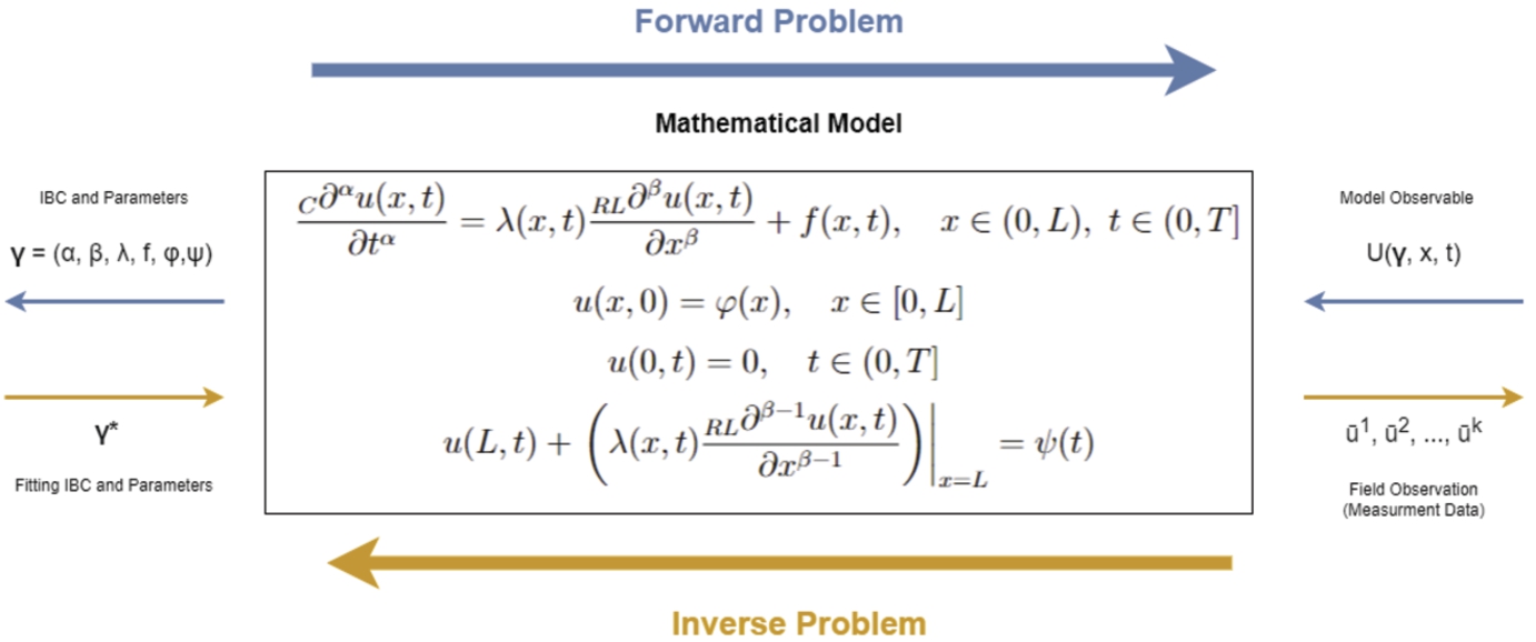
In mathematical modelling, as well as in various computer simulations it is essential to use proper mathematical models. In this paper, time-space fractional diffusion equation (TSFDE) with fractional boundary contition is considered. This model was further described in Section 2 and can be used as an effective tool in modelling the heat conduction in porous materials (Brociek et al., 2019). To solve model described by (1)–(4) it is necessary to know full information about the model input, such as material’s parameters, geometry or model coefficients. In many engineering issues, it is impossible to have the knowledge of all model’s information. It might be because of the lack of measuring equipment, or toughness in choosing the parameters. The usual problem is the choice of such entry model’s parameters – input, that the model’s result – output (e.g. temperature measurements in a chosen control point) takes the proper value. Problems of this sort are named inverse problems and are usually hard to solve (Özişik and Orlande, 2021; Aster et al., 2013c, 2013a, 2013b). To put it simply, the problem is the identifying of the input parameters to fit to the measurement data (part of model’s output) as closely as possible.

In this article, in order to solve the inverse problem, an approach is presented which involves optimizing the following fitness function:

Fig. 1

Data flow diagram for forward and inverse problem.

5Metaheuristics Optimization Algorithms

Heuristic optimization algorithms for searching objective function’s minimum are based on simulating group’s intelligence and communication between the individuals in order to effectively search the space.

They are used for finding points in search space close to the optimal one (global minimum) in terms of fitness function. Very commonly fitness function describes a certain dependence (e.g. approximate solution error), which in an engineering problem should have the lowest possible value (problem of minimization). In contrast to classic mathematical methods, they have small requirements for objective function, which is their biggest advantage. Usually, within heuristic optimization algorithms, two phases of searching can be distinguished: exploration part – searching through possibly the vastest part of space, and exploitation part – looking for good quality solutions in a narrow part of searched space. Algorithms of this sort use different techniques, from simple local searching to advanced evolutionary processes. They use mechanisms preventing the method from getting stuck in a limited area of searched space (falling into a local minimum). These algorithms are independent of a specific problem (they do not depend on the fitness function). Algorithms use knowledge about the problem and/or experience accumulated in a process of searching the domain (agents “communicate” with one another), with quality not decreasing as the iteration increases. This kind of algorithms falls into the category of probabilistic algorithms, meaning that their method of work include some random elements. However, a well-tuned algorithm in a vast majority of cases should be able to provide solutions, which are close to one another.

The biggest problem of heuristic optimization algorithms is tuning them properly, according to the problem to be solved. Metaheuristic optimization algorithms can be divided into four major groups:

These algorithms gained interest because of their effectiveness in various optimization engineering problems. Examples of their usefulness include publications (Kalita et al., 2023; Alyami et al., 2024; Zhang and Chi, 2023; Brociek and Słota, 2015). In this paper, some of metaheuristic optimization algorithms were used and compared, from which, three best (in terms of solving inverse problem for model with fractional derivative) were described in further subsections.

5.1Group Teaching Optimization

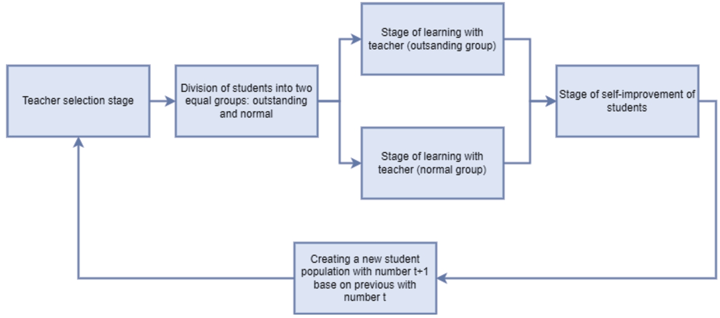
Group Teaching Optimization Algorithm (GTOA) described in this section takes inspiration from the process of group teaching. The goal of the process is to improve knowledge of the group of students. The process of teaching can be realized by different means, through learning with a teacher, exchanging knowledge between the students or self-improvement. Each student acquires knowledge with different efficiency, so it is natural to divide them into two groups: students with normal abilities and outstanding students. The teacher, in order to maximize the result, must use different methods while teaching each group. All of these mechanisms were used as an inspiration in creating Group Teaching Optimization Algorithm (Zhang and Jin, 2020).

For algorithm’s presentation, the following notation is used:

dim – dimension of the task, N – number of students in population, F – fitness function,

xit=[xi,1t,xi,2t,…,xi,dimt]	–	i-th student during iteration t before learning with a teacher,
xteachert=[xteacher,1t,xteacher,2t,…,xteacher,dimt]	–	teacher in iteration t,
xALTit=[xALTi,1t,xALTi,2t,…,xALTi,dimt]	–	i-th student after learning with teacher during iteration t,
xALSit=[xALSi,1t,xALSi,2t,…,xALSi,dimt]	–	i-th student after learning with other students during iteration t,
xAVGt=[xAVG,1t,xAVG,2t,…,xAVG,dimt]	–	average students’ knowledge within the population during iteration t,
xbestt=[xbest,1t,xbest,2t,…,xbest,dimt]	–	the best student in iteration t,
xsecondt=[xsecond,1t,xsecond,2t,…,xsecond,dimt]	–	the second best student in iterationt,
xthirdt=[xthird,1t,xthird,2t,…,xthird,dimt]	–	the third best student in iterationt.

To generalize, in a process of a group teaching, a few steps can be distinguished. Below, these steps are introduced along with their mathematical description, which make up a model of algorithm’s operation.

• • Step 1 – Choosing the teacher. During this step, a so-called teacher is chosen from the whole population. The evaluation of students in a population is determined by their fitness value – the smaller the value is, the better the quality (knowledge) of the student. The process of choosing the teacher is done on the basis of the following equation:

  (14)

  xteachert=xbestt,F(xbestt)<F(xbestt+xsecondt+xthirdt3),xbestt+xsecondt+xthirdt3,F(xbestt)⩾F(xbestt+xsecondt+xthirdt3).

• • Step 2 – Division of the students. During this step, all individuals within the population are divided into two, equally populated groups based on their knowledge (quality of their result). The results of this division are two groups, outstanding and normal groups of students.

• • Step 3 – Learning with a teacher. In case of learning with a teacher, the process differs for both of the groups created in the previous step. The teacher uses different methods for different students groups. Mathematically, this process can be described with following equations:

  for students in the outstanding group:

  (15)

  xALTit=xit+a(xteachert−fbxAVGt−fcxit),
  for students in the normal group:

  (16)

  xALTit=xit+2d(xteachert−xit).
  In equations (15), (16), symbols a, b, c, d were used to represent random numbers within the scope [0,1], symbol f represents the so-called teaching factor. In this case, f=1.

  Fig. 2

  Diagram of next steps of GTOA.

  

  If student’s knowledge increased, after the learning with a teacher, then the student goes to the next step. Otherwise, to the next step goes an individual from before learning with a teacher, that is:

  (17)

  xALTit=xALTit,F(xALTit)<F(xit),xit,F(xALTit)⩾F(xit).

• • Step 4 – self-learning of students. This step simulates students learning together during their free time. Students can share knowledge between one another and learn together, they can learn by themselves as well. The mathematical description of this process is as follows:

  (18)

  xALS,it=xALT,it+e(xALT,it−xALT,jt)+g(xALT,it−xit),forF(xALT,it)<F(xALT,jt),xALT,it−e(xALT,it−xALT,jt)+g(xALT,it−xit),forF(xALT,it)⩾F(xALT,jt).
  Symbols e, g were used to represent random number from [0,1]. Index j≠i appearing in the equation (18) represents a random student. Hence, the interaction between students i and j. Those students, who increased their knowledge after this step, pass to the next population (denoted by t+1), meaning:

  (19)

  xit+1=xALT,it,F(xALT,it)<F(xALS,it),xALS,it,F(xALT,it)⩾F(xALS,it).

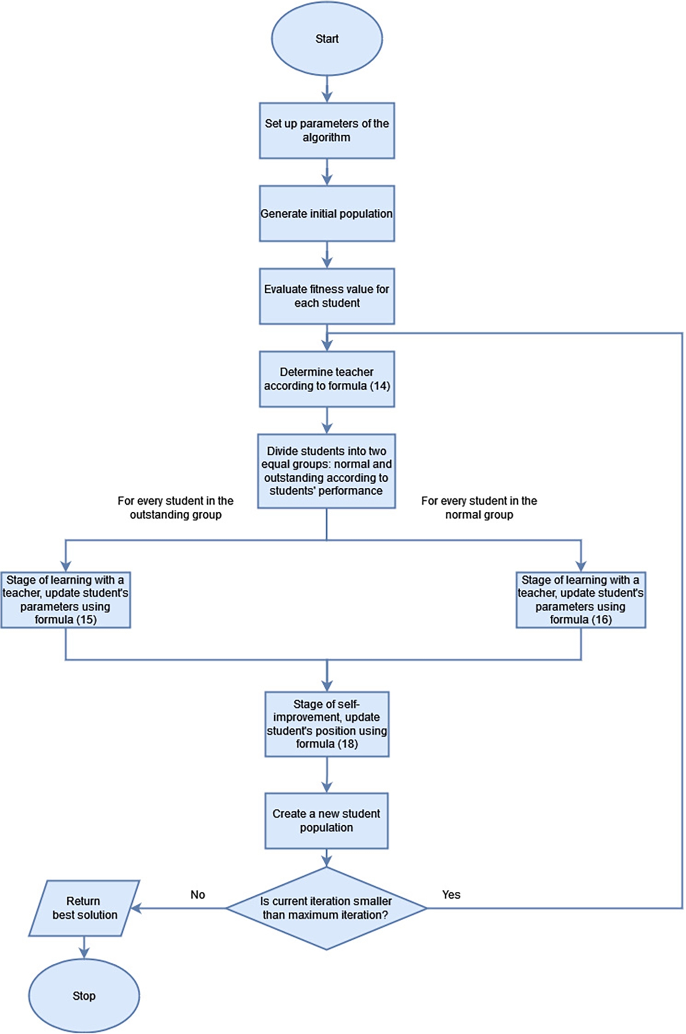
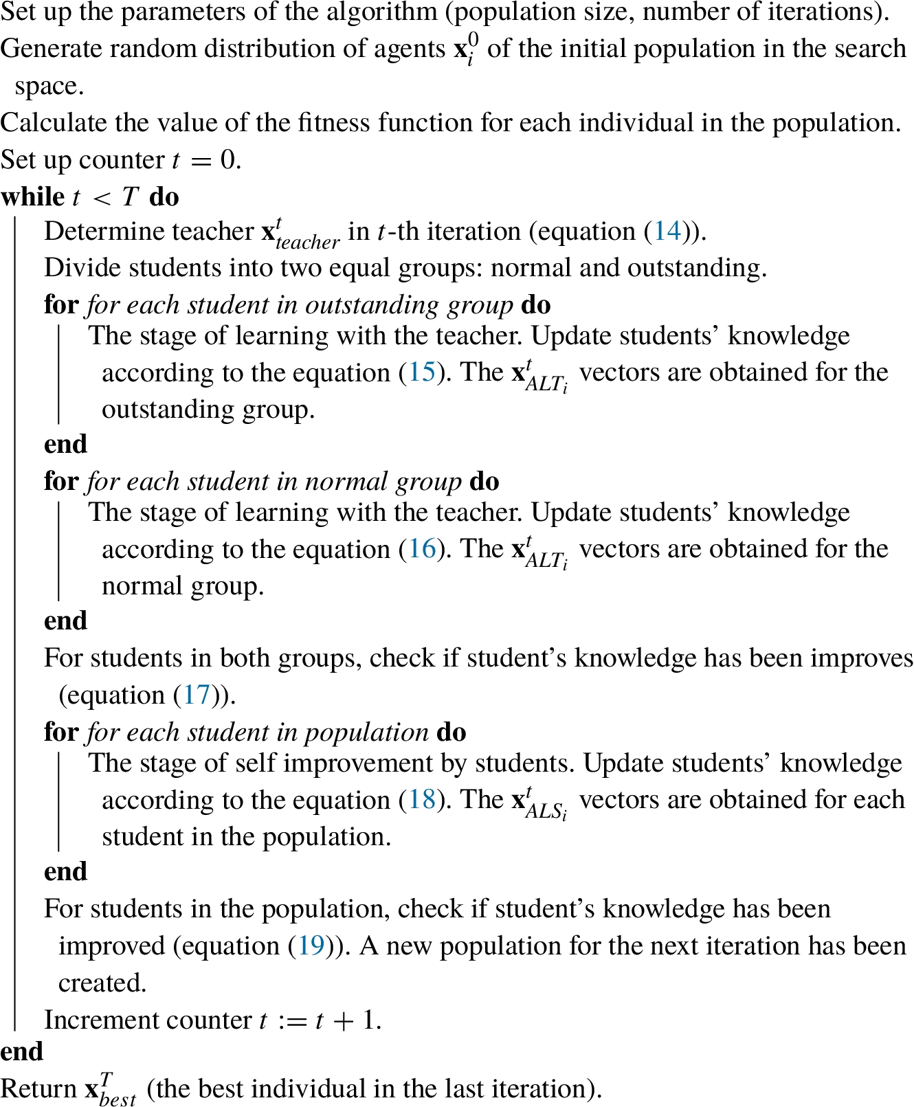
Figure 2 schematically depicts the next steps of GTOA algoritm, while Fig. 3 presents the block diagram of the algorithm. Pseudocode 1 presents the next steps of GTOA.

Fig. 3

Block diagram of GTOA.

Algorithm 1

Pseudocode of GTOA

5.2Artificial Bee Colony

Artificial Bee Colony (ABC) is one of many metaheuristic algorithms based on animals’ behaviour in their natural environment. In order to find food sources, the algorithm divides bees into two groups:

Working bees – bees that at the moment are scavenging through the already found food sources. For those bees, important factors are the distance between the source and the hive and the amount of nectar in the food source.

Unclassified bees – those bees’ mission is to search for new food sources. They can be further divided into two groups: observers and scouts. Scouts look for new food sources randomly, while observers plan their search based on the information they’re provided with.

Bees exchange information by performing a special dance. Observer bees decide how to search the space based on the dance of other bees. After the collection of nectar, every bee can decide, whether they should share information about the food source they’ve been exploring, keep on exploring it without the information exchange with other bees or discard the food source and become an observer. In order to present the ABC algorithm, a following notation has been used:

dim – dimension of the task,

N – number of bees in a colony = number of food sources,

F – fitness function, The process of an ABC algorithm can be generalized into a few steps. Below, these steps are presented together with their corresponding mathematical descriptions.

• • Step 1 – Dance. At this point scouting bees return to the hive and begin to share information about the food source they’ve been exploring. Based on the information provided by the scouts, every source is evaluated and assigned a probability according to its quality in comparison with other food sources. It is depicted by an equation below:

  (20)

  pi=fit(xi)∑j=1Nfit(xj),
  where

  (21)

  fit(xi)=11+F(xi),ifF(xi)⩾0,|1+F(xi)|,ifF(xi)<0.

• • Step 2 – Leaving the hive. After the dance ends, every observer chooses one of the food sources and sets out to explore it (one source can be chosen multiple times), the source is being modified and if the modified source is better than the original one, it replaces the original one. The formula used to modify the food source is the following:

  (22)

  vit=xit+Φi(xit−xkt).
  In the equation (22), Φi is a pseudo-random number between 0 and 1, k is a randomly selected index different than i. If the fitness value of modified food source is better than the one’s before exploration, the modified one replaces the original as a food source, otherwise it is discarded.

• • Step 3 – Abandoning old food sources. All of the sources which haven’t been chosen by any of the bees are being discarded and replaced with a new one, that is created using the following formula:

  (23)

  xi=xmin+ωi(xmax−xmin),
  where ωi is a pseudo-random number within the range [0,1] and max, min represent the upper and lower limits of the search area, respectively.

More details about the algorithm itself and its exemplary applications are presented in Li et al. (2012), Karaboga and Basturk (2007), Roeva (2018).

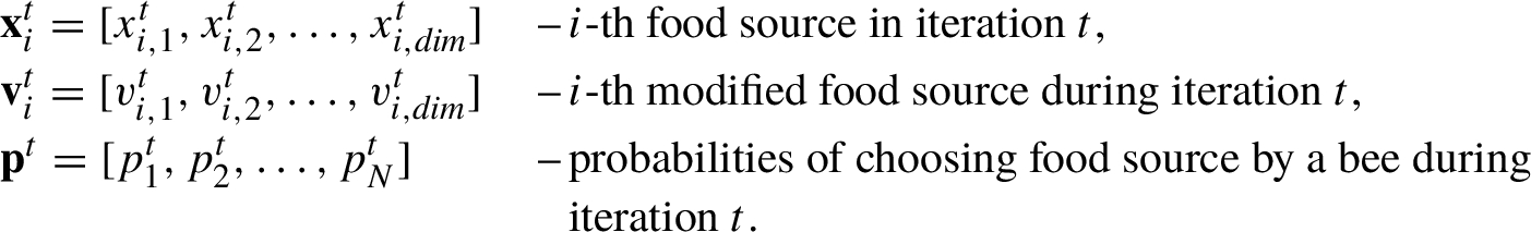
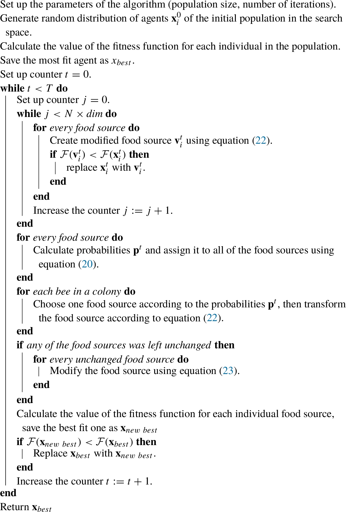
Fig. 4

Block diagram of ABC algorithm.

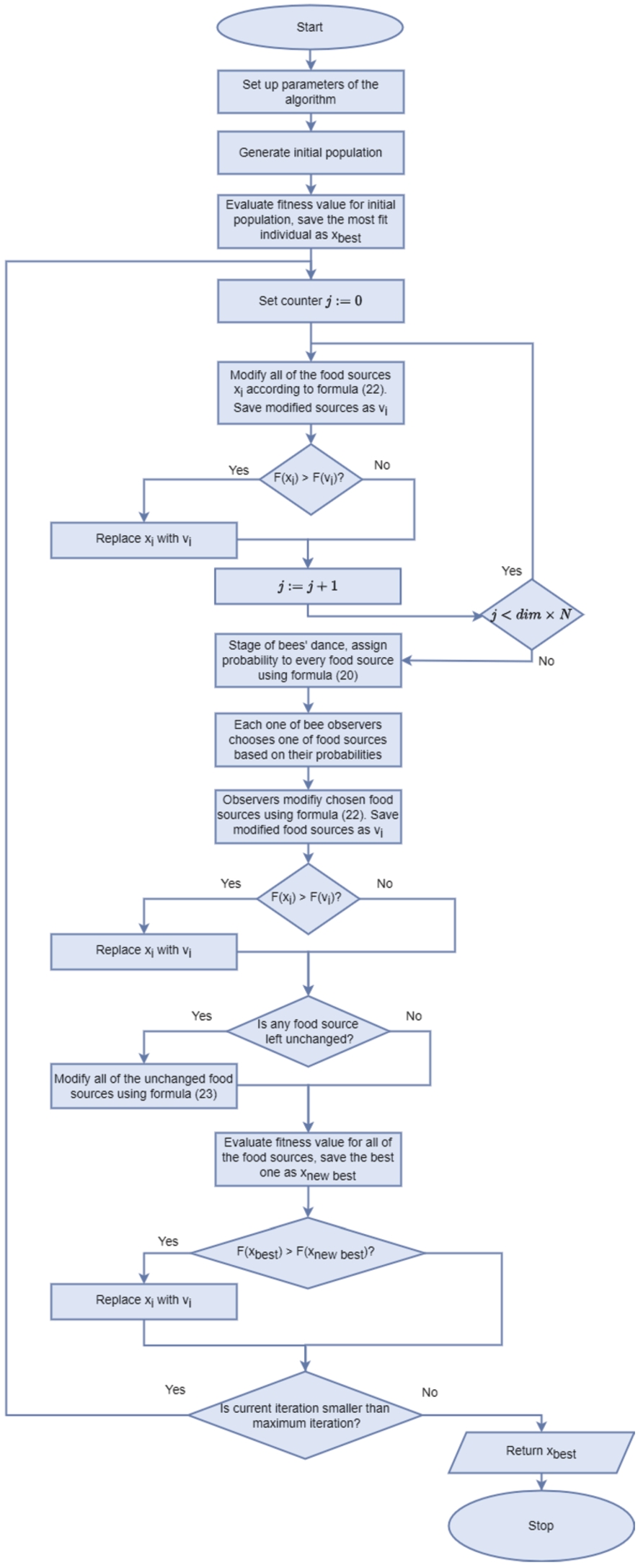
Algorithm 2

Pseudocode of ABC

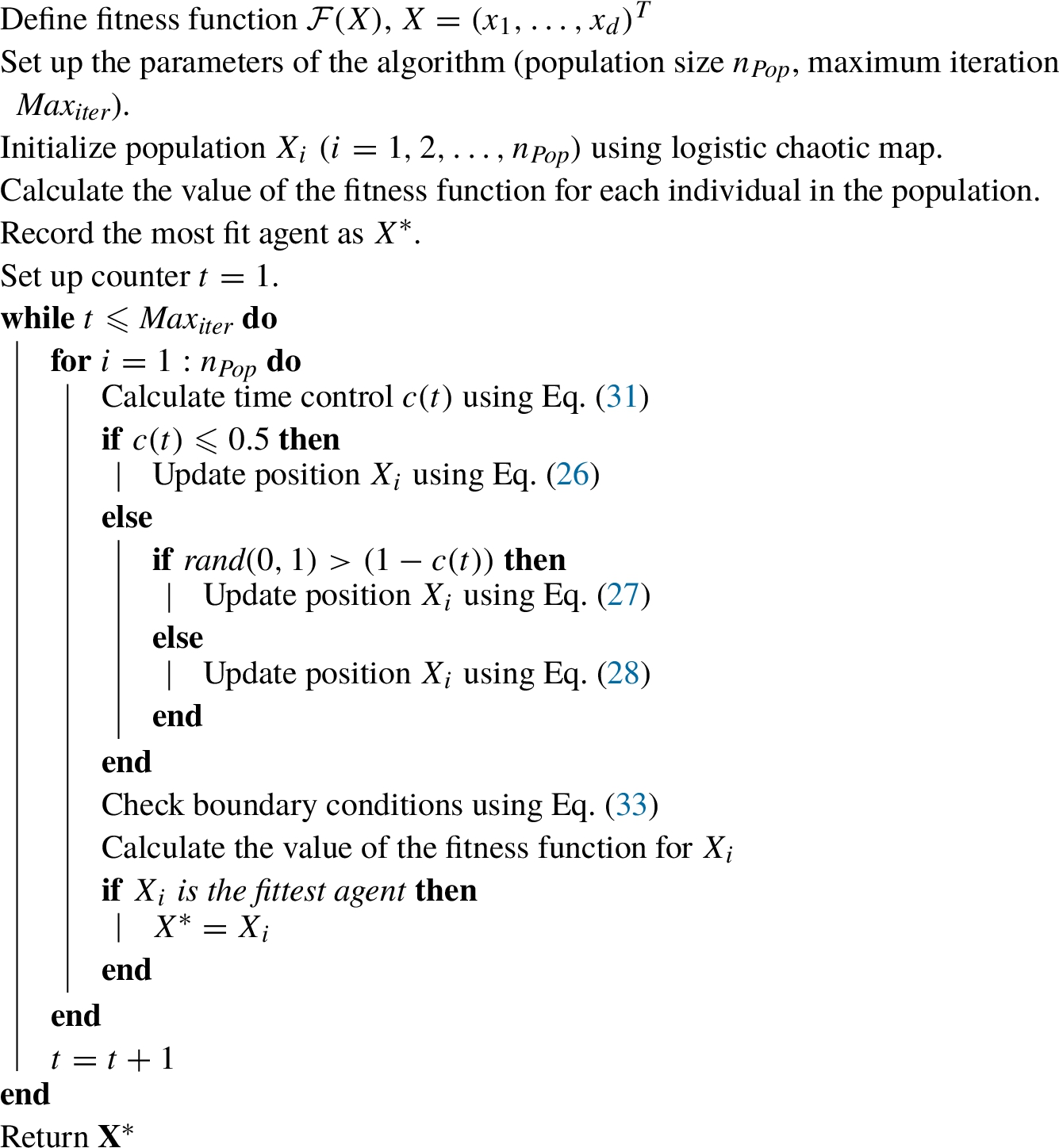
5.3Jellyfish Search

This algorithm was inspired by the behaviour of jellyfish in the ocean. It simulates factors such as following ocean currents, passive and active movements inside jellyfish swarm, time control mechanism which governs the switching between types of movement and convergence into jellyfish bloom.

Ocean Current

The direction of the ocean current is obtained by averaging all the vectors from each jellyfish in the ocean to the jellyfish that is currently in the best location:

(24)

trend→=X∗−ec∑XinPop=X∗−ecμ,

where nPop is the number of jellyfish; X∗ is the jellyfish currently with the best location in the swarm; ec is the factor that governs the attraction; μ is the mean location of all jellyfish. Because we assume that there is a normal spatial distribution of jellyfish in all dimensions, the previous equation can be transformed in the following way:

(25)

trend→=X∗−β×rand(0,1)×μ,

where β>0 is a distribution coefficient, related to the length of trend→. Based on the results of sensitivity analysis in numerical experiments carried out by authors of this algorithm, β=3 is obtained.

Finally, the new location of each jellyfish is given by:

(26)

Xi(t+1)=Xi(t)+rand(0,1)×(X∗−β×rand(0,1)×μ).

Movement Inside Swarm

After the formation of the swarm, most jellyfish exhibit type A motion. As time goes on, more and more jellyfish begin to exhibit type B motion.

• (a) Type A motions (Passive motions)

  Type A motion is the motion of jellyfish around their own locations. The new location of each jellyfish is given by

  (27)

  Xi(t+1)=Xi(t)+γ×rand(0,1)×(Ub−Lb),
  where Ub and Lb are the upper bound and lower bound of search spaces, respectively; γ=0.1 is a motion coefficient.

• (b) Type B motions (Active motions)

  To update the position of a jellyfish (i) in the type B motion, another jellyfish (j) must be selected at random. Then we compare the quantity of food at the locations of those jellyfish and create a vector from the position with less food to the position with more food. This vector is used to move jellyfish of interest (i) toward direction with more food.

  (28)

  Xi(t+1)=Xi(t)+Step→,

  (29)

  Step→=rand(0,1)×Direction→,

  (30)

  Direction→=Xj(t)−Xi(t),F(Xi)⩾F(Xj),Xi(t)−Xj(t),F(Xi)<F(Xj),
  where F is an fitness function of location X.

Time Control Mechanism

To regulate the movement of jellyfish between following the ocean current and moving inside the jellyfish swarm, the time control mechanism is introduced. It includes a time control function c(t) which is a random value that fluctuates from 0 to 1 over time.

(31)

c(t)=|(1−tMaxiter)×(2×rand(0,1)−1)|,

where t is the time specified as the iteration number and Maxiter is the maximum number of iterations, which is an initialized parameter.

To decide which type of movement to use inside a swarm, the function (1−c(t)) is used. When its value is less than rand(0,1), the jellyfish exhibits type A motion. Otherwise, the jellyfish exhibits type B motion.

Population Initialization

In order to get initial population which is more diverse and has a lower probability of premature convergence than the one with random positions, the logistic map has been used.

(32)

Xi+1=ηXi(1−Xi),0⩽X0⩽1.

Xi is the logistic chaotic value of location of the ith jellyfish; X0 is used for generating initial population of jellyfish, X0∈(0,1), X0∉{0.0,0.25,0.75,0.5,1.0}, and parameter η is set to 4.0.

Boundary Conditions

Oceans are located around the world. The earth is approximately spherical, so when a jellyfish moves outside the bounded search area, it will return to the opposite bound.

(33)

X′i,d=(Xi,d−Lb,d)+Lb(d),Xi,d>Lb,d,(Xi,d−Ub,d)+Ub(d),Xi,d<Ub,d.

Xi,d is the location of the ith jellyfish in dth dimension; X′i,d is the updated location after checking boundary constraints. Ub,d and Lb,d are upper and lower bounds of dth dimension in search spaces, respectively.

More details about the JS and its exemplary applications are presented in the publications (Chou and Truong, 2021; Bujok, 2021; Youssef et al., 2021).

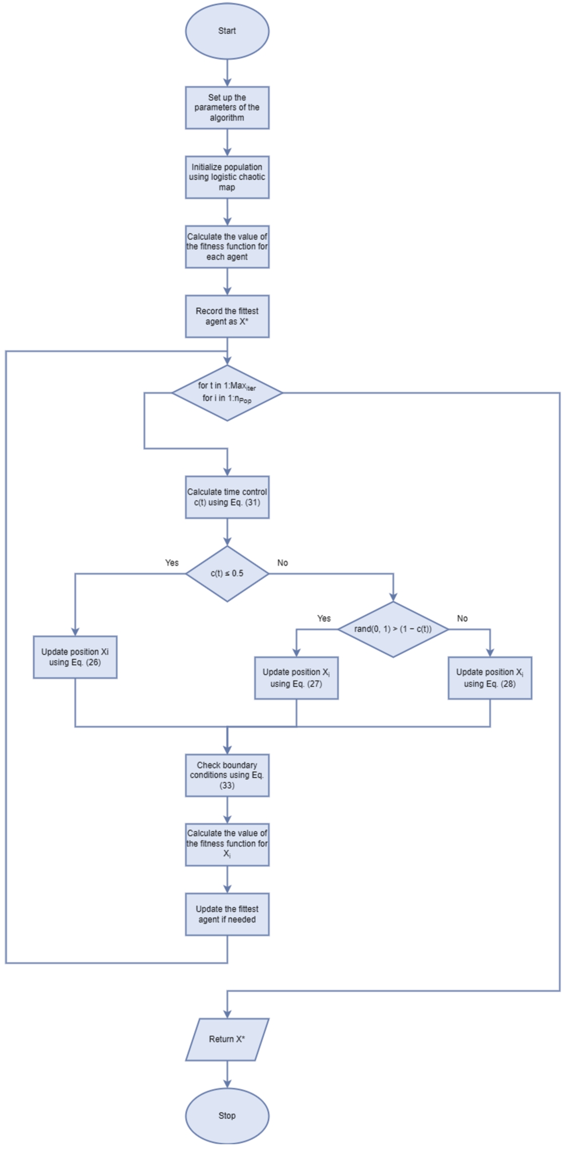
Fig. 5

Block diagram of JS.

Algorithm 3

Pseudocode of JS

6Computational Example

This section is designed to present how the presented method of solving an inverse problem for the model of anomalous diffusion works. As an example, the results provided by a few chosen metaheuristic optimization algorithms were compared.

In a considered inverse problem, fractional boundary condition (4) on the right side is recreated, specifically, function ψ appearing in mentioned condition, as well as orders of fractional derivatives α, β. In the model (1)–(4), the following numeric data was assumed:

Data necessary for solving the inverse problem is value of the function u in control point xp=1 (the right boundary). This data was generated as a result of solving the direct problem for the measurement grid 400×400. During the algorithm’s work on solving the inverse problem, grid of the size 100×200 was used. Using different sizes of grid is for evading the phenomena known as inverse crime (Kaipio and Somersalo, 2005). To find the minimum of fitness function (13), which describes the error of approximated solution, selected metaheuristic optimization algorithms were used. Tested group of algorithms includes described in the Section 5 Group Teaching Optimization Algorithm (GTOA), Artificial Bee Colony (ABC) and Jellyfish Search (JS). Apart from previously mentioned, following heuristics were used: Equilibrium Optimizer (EO), Grey Wolf Optimizer (GWO), War Strategy Optimization (WSO), Tuna Swarm Optimization (TSO) and Ant Colony Optimization (ACO). In each algorithm, values of parameters such as number of iterations and size of the population were chosen in a way that ensures similar number of calls of fitness function. This is to compare the results obtained from these algorithms.

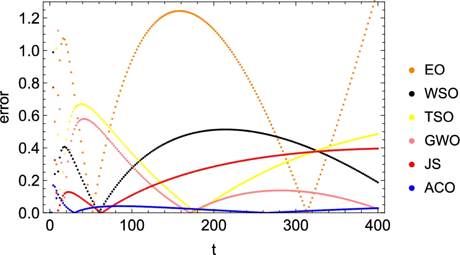
Obtained results of the search of the minimum of fitness function are presented in a Table 2. Colour blue was used to mark three algorithms (GTOA, ABC and JS), which returned a satisfying result. Colour red was used to mark the rest of the algorithms, which did not handle the task so well. Smallest value of objective function was achieved for GTOA and was approximately 0.007. Also, in this case, errors of identifying parameters a0,a1,…,a6 are the smallest. Similarly for ABC and JS, obtained errors and value of objective function are on acceptable level. It is also worth to pay attention to the results from ACO, where value of fitness function is low. However, the errors in identification of parameters are on an unacceptable level, which proves that the algorithm got stuck in a local minimum. For other algorithms,a the values of objective function are on a relatively highly level.

Table 2

Results of parameters identification, a‾i – identified value of ai coefficient, Δa‾i – absolute error of identification, δa‾i – relative error of identification, F – value of fitness function.

Another important indicator is fitness of data from control point (so called measurement data) to data obtained from model. On one hand, the measure determining this fit is the value of the objective function F, while on the other hand, it is the errors of the reconstructed function u for the identified parameters. Figures 6 (for GTOA and ABC) and 7 (for other algorithms) present errors of distribution of the recreated function u in a control point. For the two best algorithms (GTOA and ABC), these errors are much smaller (≈10−2) than for the rest of the algorithms (≈101) (see Figs. 6, 7).

Fig. 6

Errors distribution in a control point for GTOA and ABC algorithms.

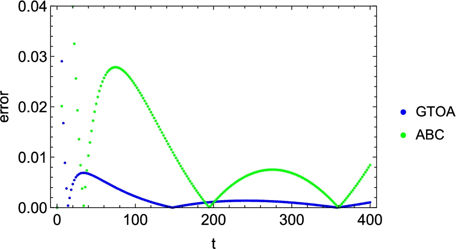
Fig. 7

Error distribution in a control point for EO, WSO, TSO, GWO, JS, ACO algorithms.

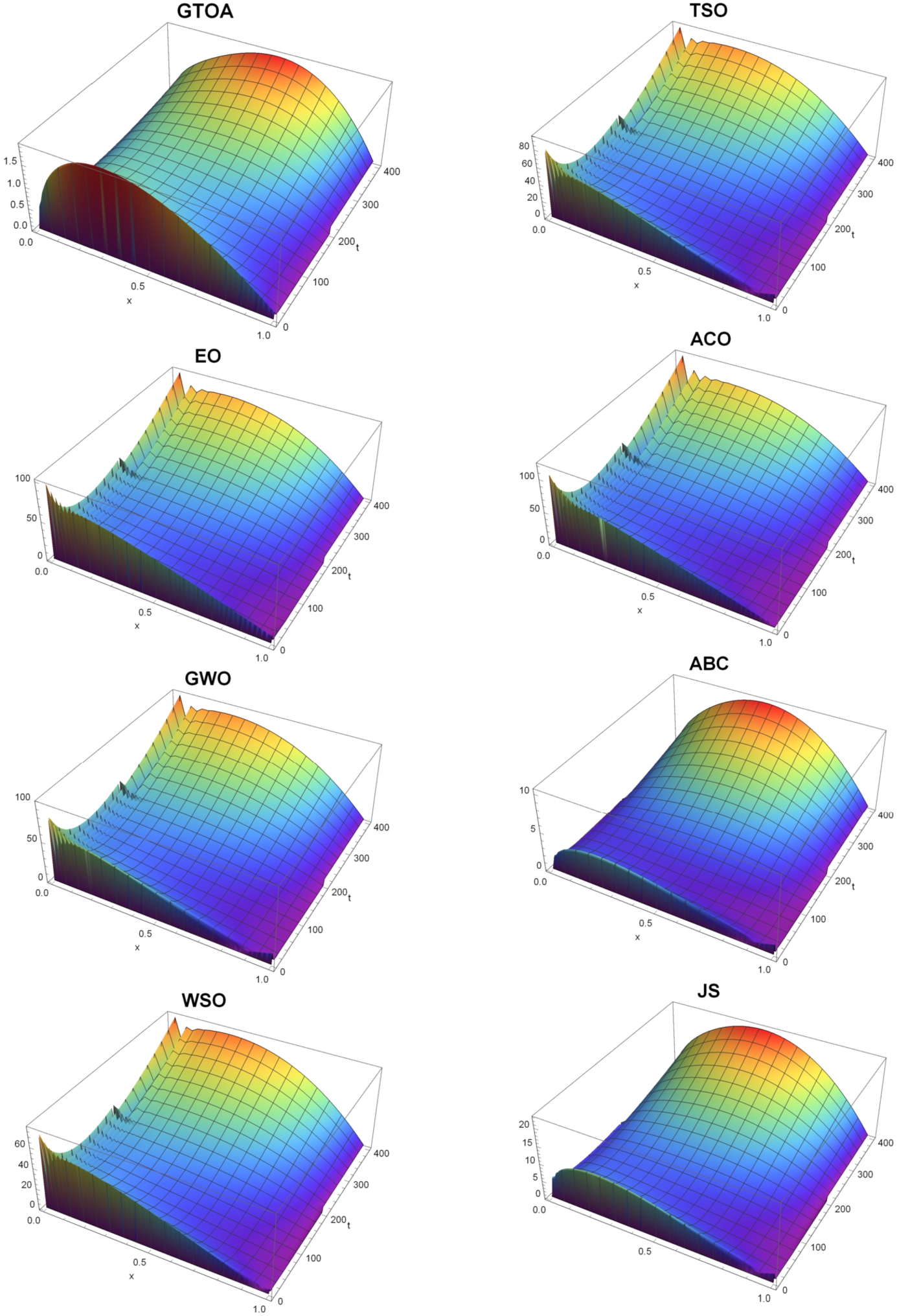
Because the exact solution is known, we decided to calculate the errors of reconstruction function u in a full domain (not only in control point). In Fig. 8 errors of reconstruction function u for identified model parameters are presented. For three best algorithms, these errors are on an acceptable level and they share similar characteristics. It is the case of GTOA (maximum error ≈1.5), ABC (maximum error ≈10) and JS (maximum error ≈20). In the rest of algorithms, maximum errors are high and unacceptable.

Fig. 8

Function u’s reconstruction’s error in a full domain.

As part of the conducted computations, a comparison of the error of identification of the function ψ occurring in the boundary condition was also performed. These errors were calculated using the formula:

7Conclusion

This article focuses on the method of solving the inverse problem for diffusion equation with fractional derivatives. In the considered task, the orders of derivatives and the function occurring in the boundary condition were identified. In the presented approach, the forward problem was solved using an implicit finite difference scheme, while the inverse problem was solved using heuristic optimization algorithms. The inverse problem turned out to be difficult to solve and required identification of seven parameters.

To solve the inverse problem, the following metaheuristic algorithms were compared: GTOA, ABC, ACO, EO, GWO, JS, TSO, WSO. Satisfactory results were obtained for the Group Teaching Optimization Algorithm (GTOA) and the Artificial Bee Colony (ABC) method. Additionally, the Jellyfish Search (JS) algorithm yielded an acceptable result. The remaining algorithms proved unsuitable for this type of problem.

One of the conclusions from the conducted research and next step in the research is the possibility to build a hybrid algorithm. Firstly, a heuristic algorithm could be used for initial solution localization (exploration part), while deterministic methods such as Nelder-Mead or Hooke-Jeeves could be employed for more focused searches (eploitation part). This is the next step and a plan for future research in the work carried out by the authors of this paper.

References

1 | Al Thobiani, F., Khatir, S., Benaissa, B., Ghandourah, E., Mirjalili, S., Abdel Wahab, M. ((2022) ). A hybrid PSO and Grey Wolf Optimization algorithm for static and dynamic crack identification. Theoretical and Applied Fracture Mechanics, 118: , 103213. https://doi.org/10.1016/j.tafmec.2021.103213. |
2 | Alyami, M., Khan, M., Javed, M.F., Ali, M., Alabduljabbar, H., Najeh, T., Gamil, Y. ((2024) ). Application of metaheuristic optimization algorithms in predicting the compressive strength of 3D-printed fiber-reinforced concrete. Developments in the Built Environment, 17: , 100307. https://doi.org/10.1016/j.dibe.2023.100307. |
3 | Arul, R., Karthikeyan, P., Karthikeyan, K., Geetha, P., Alruwaily, Y., Almaghamsi, L., El-hady, E.-S. ((2022) ). On Ψ-Hilfer fractional integro-differential equations with non-instantaneous impulsive conditions. Fractal and Fractional, 6: (12). https://doi.org/10.3390/fractalfract6120732. |
4 | Ashurov, R., Kadirkulov, B., Ergashev, O. ((2023) ). Inverse problem of Bitsadze–Samarskii type for a two-dimensional parabolic equation of fractional order. Journal of Mathematical Sciences (United States), 274: (2), 172–185. https://doi.org/10.1007/s10958-023-06587-8. |
5 | Aster, R.C., Borchers, B., Thurber, C.H. ((2013) a). Chapter four – Tikhonov regularization. In: Aster, R.C., Borchers, B., Thurber, C.H. (Eds.), Parameter Estimation and Inverse Problems, second ed. Academic Press, Boston, pp. 93–127. 978-0-12-385048-5. https://doi.org/10.1016/B978-0-12-385048-5.00004-5. |
6 | Aster, R.C., Borchers, B., Thurber, C.H. ((2013) b). Chapter ten – Nonlinear inverse problems. In: Aster, R.C., Borchers, B., Thurber, C.H. (Eds.), Parameter Estimation and Inverse Problems, second ed. Academic Press, Boston, pp. 239–252. 978-0-12-385048-5. https://doi.org/10.1016/B978-0-12-385048-5.00010-0. |
7 | Aster, R.C., Borchers, B., Thurber, C.H. ((2013) c). Chapter three – Rank deficiency and Ill-conditioning. In: Aster, R.C., Borchers, B., Thurber, C.H. (Eds.), Parameter Estimation and Inverse Problems, second ed. Academic Press, Boston, pp. 55–91. 978-0-12-385048-5. https://doi.org/10.1016/B978-0-12-385048-5.00003-3. |
8 | Bhangale, N., Kachhia, K.B., Gómez-Aguilar, J.F. ((2023) ). Fractional viscoelastic models with Caputo generalized fractional derivative. Mathematical Methods in the Applied Sciences, 46: (7), 7835–7846. https://doi.org/10.1002/mma.7229. |
9 | Bohaienko, V., Gladky, A. ((2023) ). Modelling fractional-order moisture transport in irrigation using artificial neural networks. SeMA Journal, 81: , 219–233. https://doi.org/10.1007/s40324-023-00322-8. |
10 | Brociek, R., Słota, D. ((2015) ). Application of intelligent algorithm to solve the fractional heat conduction inverse problem. Communications in Computer and Information Science, 538: , 356–365. https://doi.org/10.1007/978-3-319-24770-0_31. |
11 | Brociek, R., Słota, D., Król, M., Matula, G., Kwaśny, W. ((2017) ). Modeling of heat distribution in porous aluminum using fractional differential equation. Fractal and Fractional, 1: (1), 17. |
12 | Brociek, R., Słota, D., Król, M., Matula, G., Kwaśny, W. ((2019) ). Comparison of mathematical models with fractional derivative for the heat conduction inverse problem based on the measurements of temperature in porous aluminum. International Journal of Heat and Mass Transfer, 143: , 118440. |
13 | Brociek, R., Chmielowska, A., Słota, D. ((2020) ). Comparison of the probabilistic ant colony optimization algorithm and some iteration method in application for solving the inverse problem on model with the caputo type fractional derivative. Entropy, 22: (5), 555. https://doi.org/10.3390/E22050555. |
14 | Brociek, R., Wajda, A., Capizzi, G., Słota, D. ((2023) ). Parameter estimation in the mathematical model of bacterial colony patterns in symmetry domain. Symmetry, 15: (4), 782. https://doi.org/10.3390/sym15040782. |
15 | Brociek, R., Hetmaniok, E., Napoli, C., Capizzi, G., Słota, D. ((2024) ). Identification of aerothermal heating for thermal protection systems taking into account the thermal resistance between layers. International Journal of Heat and Mass Transfer, 218: , 124772. https://doi.org/10.1016/j.ijheatmasstransfer.2023.124772. |
16 | Bujok, P. ((2021) ). Three steps to improve jellyfish search optimiser. MENDEL, 27: (1), 29–40. https://doi.org/10.13164/mendel.2021.1.029. |
17 | Chou, J.-S., Truong, D.-N. ((2021) ). A novel metaheuristic optimizer inspired by behavior of jellyfish in ocean. Applied Mathematics and Computation, 389: , 125535. https://doi.org/10.1016/j.amc.2020.125535. |
18 | Ciesielski, M., Grodzki, G. ((2023) ). Numerical Approximations of the Riemann–Liouville and Riesz fractional integrals. Informatica, 389: (1), 21–46 . https://doi.org/10.15388/23-INFOR540. |
19 | Hassan, H., Tallman, T.N. ((2021) ). A comparison of metaheuristic algorithms for solving the piezoresistive inverse Problem in self-sensing materials. IEEE Sensors Journal, 21: (1), 659–666. https://doi.org/10.1109/JSEN.2020.3014554. |
20 | Hou, J., Meng, X., Wang, J., Han, Y., Yu, Y. ((2023) ). Local error estimate of an L1-finite difference scheme for the multiterm two-dimensional time-fractional reaction-diffusion equation with robin boundary conditions. Fractal and Fractional, 7: (6), 453. https://doi.org/10.3390/fractalfract7060453. |
21 | Hristov, J. ((2023) a). Chapter 11 – Fourth-order fractional diffusion equations: constructs and memory kernel effects. In: Baleanu, D., Balas, V.E., Agarwal, P. (Eds.), Fractional Order Systems and Applications in Engineering, Advanced Studies in Complex Systems. Academic Press, pp. 199–214. 978-0-323-90953-2. https://doi.org/10.1016/B978-0-32-390953-2.00019-0. |
22 | Hristov, J. ((2023) b). Special issue “Trends in fractional modelling in science and innovative technologies”. Symmetry, 15: (4), 884. https://doi.org/10.3390/sym15040884. |
23 | Ibraheem, Q.W., Hussein, M.S. ((2023) ). Determination of time-dependent coefficient in time fractional heat equation. Partial Differential Equations in Applied Mathematics, 7: (12), 100492. https://doi.org/10.1016/j.padiff.2023.100492. |
24 | Ionescu, C., Lopes, A., Copot, D., Machado, J.A.T., Bates, J.H.T. ((2017) ). The role of fractional calculus in modeling biological phenomena: a review. Communications in Nonlinear Science and Numerical Simulation, 51: , 141–159. https://doi.org/10.1016/j.cnsns.2017.04.001. |
25 | Kaipio, J., Somersalo, E. ((2005) ). Statistical and Computational Inverse Problems. Springer, New York. |
26 | Kalita, K., Ganesh, N., Shankar, R., Chakraborty, S. ((2023) ). A fuzzy MARCOS-based analysis of dragonfly algorithm variants in industrial optimization problems. Informatica, 35: (1), 155–178. https://doi.org/10.15388/23-INFOR538. |
27 | Karaboga, D., Basturk, B. ((2007) ). Artificial Bee Colony (ABC) optimization algorithm for solving constrained optimization problems. In: Melin, P., Castillo, O., Aguilar, L.T., Kacprzyk, J., Pedrycz, W. (Eds.), Foundations of Fuzzy Logic and Soft Computing. Springer Berlin Heidelberg, Berlin, Heidelberg, pp. 789–798. 978-3-540-72950-1. |
28 | Koleva, M.N., Poveschenko, Y., Vulkov, L.G. ((2021) ). Numerical simulation of thermoelastic nonlinear waves in fluid saturated porous media with non-local Darcy law. In: Dimov, I., Fidanova, S. (Eds.), Advances in High Performance Computing. Springer International Publishing, Cham, pp. 279–289. 978-3-030-55347-0. |
29 | Kukla, S., Siedlecka, U., Ciesielski, M. ((2022) ). Fractional order dual-phase-lag model of heat conduction in a composite spherical Medium. Materials, 15: (20), 7251. |
30 | Li, G., Niu, P., Xiao, X. ((2012) ). Development and investigation of efficient artificial bee colony algorithm for numerical function optimization. Applied Soft Computing, 12: (1), 320–332. https://doi.org/10.1016/j.asoc.2011.08.040. |
31 | Lin, Y., Xu, C. ((2007) ). Finite difference/spectral approximations for the time-fractional diffusion equation. Journal of Computational Physics, 225: (2), 1533–1552. https://doi.org/10.1016/j.jcp.2007.02.001. |
32 | Magacho, E.G., Jorge, A.B., Gomes, G.F. ((2023) ). Inverse problem based multiobjective sunflower optimization for structural health monitoring of three-dimensional trusses. Evolutionary Intelligence, 16: (1), 247–267. https://doi.org/10.1007/s12065-021-00652-4. |
33 | Montazeri, M., Mohammadiun, H., Mohammadiun, M., Bonab, D., Hossein, M., Vahedi, M. ((2022) ). Inverse estimation of time-dependent heat flux in stagnation region of annular jet on a cylinder using Levenberg–Marquardt method. Iranian Journal of Chemistry and Chemical Engineering, 41: (3), 971–988. https://doi.org/10.30492/ijcce.2021.131987.4263. |
34 | Obembe, A.D., Al-Yousef, H.Y., Hossain, M.E., Abu-Khamsin, S.A. ((2017) ). Fractional derivatives and their applications in reservoir engineering problems: a review. Journal of Petroleum Science and Engineering, 157: , 312–327. https://doi.org/10.1016/j.petrol.2017.07.035. |
35 | Özişik, M.N., Orlande, H.R.B. ((2021) ). Inverse Heat Transfer Fundamentals and Applications. Taylor and Francis Group. |
36 | Podlubny, I. ((1999) ). Fractional Differential Equations. Academic Press, San Diego. |
37 | Roeva, O. ((2018) ). Application of artificial Bee Colony Algorithm for model parameter identification. In: Zelinka, I., Vasant, P., Duy, V.H., Dao, T.T. (Eds.), Innovative Computing, Optimization and Its Applications: Modelling and Simulations. Springer International Publishing, Cham, pp. 285–303. 978-3-319-66984-7. https://doi.org/10.1007/978-3-319-66984-7_17. |
38 | Sobhani, H., Azimi, A., Noghrehabadi, A., Mozafarifard, M. ((2023) ). Numerical study and parameters estimation of anomalous diffusion process in porous media based on variable-order time fractional dual-phase-lag model. Numerical Heat Transfer, Part A: Applications, 83: (7), 679–710. https://doi.org/10.1080/10407782.2022.2157915. |
39 | Sowa, M., Łukasz Majka, Wajda, K. ((2023) ). Excitation system voltage regulator modeling with the use of fractional calculus. AEU – International Journal of Electronics and Communications, 159: , 154471. https://doi.org/10.1016/j.aeue.2022.154471. |
40 | Stanisławski, R. ((2022) ). Fractional systems: state-of-the-art. Studies in Systems, Decision and Control, 402: , 3–25. https://doi.org/10.1007/978-3-030-89972-1_1. |
41 | Tadjeran, C., Meerschaert, M.M. ((2007) ). A second-order accurate numerical method for the two-dimensional fractional diffusion equation. Journal of Computational Physics, 220: (2), 813–823. https://doi.org/10.1016/j.jcp.2006.05.030. |
42 | Tian, W., Zhou, H., Deng, W. ((2015) ). A class of second order difference approximations for solving space fractional diffusion equations. Mathematics of Computation, 84: (294), 1703–1727. |
43 | Wang, S., Li, Y., Zhou, Y., Peng, G., Xu, W. ((2023) ). Identification of thermal conductivity of transient heat transfer systems based on an improved artificial fish swarm algorithm. Journal of Thermal Analysis and Calorimetry, 148: (14), 6969–6987. https://doi.org/10.1007/s10973-023-12182-5. |
44 | Xie, C., Fang, S. ((2020) ). Finite difference scheme for time-space fractional diffusion equation with fractional boundary conditions. Mathematical Methods in the Applied Sciences, 43: (6), 3473–3487. https://doi.org/10.1002/mma.6132. |
45 | Youssef, H., Hassan, M.H., Kamel, S., Elsayed, S.K. ((2021) ). Parameter estimation of single phase transformer using Jellyfish search optimizer algorithm. In: 2021 IEEE International Conference on Automation/XXIV Congress of the Chilean Association of Automatic Control (ICA-ACCA), pp. 1–4. https://doi.org/10.1109/ICAACCA51523.2021.9465279. |
46 | Zhang, Y., Jin, Z. ((2020) ). Group teaching optimization algorithm: a novel metaheuristic method for solving global optimization problems. Expert Systems with Applications, 148: , 113246. https://doi.org/10.1016/j.eswa.2020.113246. |
47 | Zhang, Y., Chi, A. (2023). Group teaching optimization algorithm with information sharing for numerical optimization and engineering optimization. Journal of Intelligent Manufacturing, 1547–1571. https://doi.org/10.1007/s10845-021-01872-2. |