
A Two-Index Formulation for the Fixed-Destination Multi-Depot Asymmetric Travelling Salesman Problem and Some Extensions
Abstract
We introduce a compact formulation for the fixed-destination multi-depot asymmetric travelling salesman problem (FD-mATSP). It consists of m salesmen distributed among D depots who depart from and return to their respective origins after visiting a set of customers. The proposed model exploits the multi-depot aspect of the problem by labelling the arcs to identify the nodes that belong to the same tour. Our experimental investigation shows that the proposed-two index formulation is versatile and effective in modelling new variations of the FD-mATSP compared with existing formulations. We demonstrate this by applying it for the solution of two important extensions of the FD-mATSP that arise in logistics and manufacturing environments.
1Introduction
Routing problems are combinatorial optimization problems that are concerned with designing a set of routes for a fleet of salesmen or vehicles, in order to satisfy customer demand. These problems have broad applicability in industry and constitute the core of the transportation and logistics companies. Two of the most common routing problems are the travelling salesman problem (TSP) (Lawler et al., 1985; Laporte, 1992a; Reinelt, 1994; Davendra, 2010) and the vehicle routing problem (VRP) (Laporte, 1992b; Toth and Vigo, 2002; Golden et al., 2008; Kumar and Panneerselvam, 2012). They are also two of the most challenging problems to solve.
In recent years, several interesting studies have considered a fleet of salesmen or vehicles to be located at several depots from where requests or distribution of goods to customers is made (Montoya-Torres et al., 2015; Ramos et al., 2020). Multi-depot routing problems can be classified as non-fixed-destination (where the salesmen or vehicles can return to any depot) or as fixed-destination (where the vehicles return to their starting points) (Bektaş, 2012). For a review of work on multi-depot routing problems, please see Montoya-Torres et al. (2015).
The case of fixed-destination in multi-depot routing problems is an important feature that has been studied in different applications. These include the fixed-destination multiple travelling salesman problems (Burger et al., 2018), the symmetric generalized multiple-depot multiple travelling salesman problem (Malik et al., 2007), the postal distribution problem, the less-than-truckload transport operations, and balance billing-cycle vehicle routing problems (Bektaş, 2012).
In this paper, we study the fixed-destination multi-depot asymmetric travelling salesman problem (FD-mATSP), which can be defined as follows: Given a complete graph with vertex set
Less than a handful of compact formulations for the FD-mATSP are reported in the literature. Typically, these formulations incorporate three components: routing, subtour elimination constraints (SECs), and fixed-destination constraints (FDCs). The first component enforces vehicles to depart and return to the depots after visiting each client exactly once, while the second component prohibits cycles in the solution. The last component ensures that the salesmen return to their origins. Kara and Bektaş (2006) used a set of three-index binary variables to capture the routing and fixed-destination components. Then, Bektaş (2012) introduced a set of two-index binary variables to capture the routing part and a set of three-index continuous variables to model the fixed-destination component. Later, Burger et al. (2018) extended the work presented in Burger (2014) and introduced a set of two-index binary variables to capture the routing of vehicles and an additional novel set of two-index variables to label the nodes in order to identify the ones belonging to the same tour, and thereby enforcing the fixed-destination requirements.
In this paper, we formulate a new model for the FD-mATSP, which exploits the multi-depot aspect of the problem and uses two-index variables to label the arcs in order to enforce the fixed-destination requirement, which was motivated by the work reported in Aguayo (2016). Bektaş et al. (2020) have independently developed this formulation for the FDCs. We call this formulation the “arc labelled formulation” (ALF). Bektaş et al. (2020) also propose a “path labelled formulation” (PLF). However, in this paper, we consider only the ALF because of the inapplicability of the PLF to the variants of the FD-mATSP that we address. For a relative performance of these two formulations to solve the FD-mATSP, see Bektaş et al. (2020). In this paper, we present a computational investigation on the performance of the ALF, the two-index formulation of Burger et al. (2018), and the three-index formulation of Bektaş (2012) to capture the FDCs, along with some underlying insights. The two variants of the FD-mATSP that we consider are as follows. In the first variant, the nodes are split into pick-up customers and delivery customers. Each depot has only one capacitated vehicle available and an initial inventory of a product. The quantities collected from pick-up customers can be supplied to any delivery customer. Also, a transshipment is allowed at pick-up customizer locations, while a delivery customer is visited only once. The problem is to determine vehicle routes to meet customer demands with vehicles not exceeding their respective capacities and returning to their starting depots after incurring minimum total cost. In the second variant, given a set of identical vehicles at each depot, which might differ in number, a set of customers with known quantities of products for pick-up, and a set of transfer points to enable transfer of products among vehicles, the problem is to determine vehicle routes to pick up products from all the customers such that the vehicles return to their starting depots and the total cost incurred is minimized.
The remainder of this paper is organized as follows. In Section 2, we present the existing and proposed formulations for the FD-mATSP. In Section 3, we extend our formulation to two new variants of the FD-mATSP in order to show its versatility. In Section 4, we present results of our computational investigation of the proposed formulation. Concluding remarks are made in Section 5.
2Mathematical Formulations for the FD-mATSP
In this section, we first present a general formulation for the FD-mATSP in Section 2.1, while in Section 2.2, we present some pertinent polynomial-length subtour elimination constraints (SECs). We present a three-index formulation due to Bektaş et al. (2020) and a two-index formulation due to Burger et al. (2018) for the FD-mATSP in Section 2.3. And finally, we introduce our compact two-index formulation for the FD-mATSP in Section 2.4.
2.1General Formulations for the FD-mATSP
First, consider the following notation. Let D be the set of depots,
We define the following decision variable. Let
(1)
(2)
(3)
(4)
(5)
(6)
(7)
(8)
(9)
2.2Compact SECs
Letting
(10)
(11)
(12)
(13)
Letting
(14)
(15)
(16)
(17)
(18)
(19)
2.3Compact FDCs
Let
(20)
(21)
(22)
(23)
(24)
Letting
(25)
(26)
(27)
(28)
2.4Proposed FDCs
Letting
(29)
(30)
(31)
(32)
(33)
Lemma 1.
FDCs3 is equivalent to FDCs1.
Proof.
We prove this claim by verifying the equivalence between FDCs1 and FDCs3. If we let
From now on, we will use the following notation to refer to different formulations. Note that in all cases we use the GG-SECs, (14)–19, since they outperform or perform similarly than the other SECs.
MCF: refers to the multi-commodity formulation reported in Bektaş (2012) based on FDCs1; (1)–(7), (14)–(19), (20)–(24).
NLF: indicates the node-labelling formulation presented in Burger et al. (2018) based on FDCs2; (1)–(7), (14)–(19), (25)–(28).
ALF: denotes the arc-labelling formulation introduced in this paper based on FDCs3; (1)–(7), (14)–(19), (29)–(33).
Lemma 2.
The (LP) relaxation of none of the formulations ALF, NLF, and MCF is tighter than the other.
Proof.
We prove this claim by showing that any of these formulations dominates the other depending upon the problem instance considered. We refer to the LP relaxation results for these formulations presented in Table 6. For Instance ftv47, (
Regarding ALF and MCF, for Instance ftv47, the LP bound of MCF is strictly larger than that of ALF. However, for Instance ftv55 the LP bound of ALF is strictly larger than of MCF.
As regards MCF and NLF, again for Instance ftv47, the LP bound of MCF is strictly larger than that of NLF. However, for Instance ftv55 the LP bound of NLF is strictly larger than that of MCF. □
3Extensions of the FD-mATSP
In this section, we present two extensions of the FD-mATSP to illustrate the versatility and computational effectiveness of the two-index compact formulation (ALF) compared with the ones reported in the literature. To that end, we consider the fixed-destination multiple-vehicle routing problem with transshipment (FD-mVRPT), and the fixed-destination multi-depot collection problem with transfer points (FD-mDCPTP).
3.1FD-mVRPT
The FD-mVRPT can be defined as follows. We have a set of D depots each having exactly one capacitated vehicle with an initial inventory of a product, a set of P pickup customers supplying units of a product, and a set E of delivery customers demanding units of a product. The quantities collected from pickup customers can be supplied to any delivery customer. Furthermore, a transshipment is allowed, i.e. units can be transferred among vehicles at pickup customers, while the delivery customers must be visited exactly once. The problem consists of determining a set of routes so that the total cost is minimized in such a way that the delivery customers receive the amount demanded, the vehicle capacity is never exceeded, and vehicles return to their respective starting points. The FD-mVRPT can be viewed as a variant of diverse routing problems encountered in real-life applications such as the swapping problem wherein vehicles transport objects among customers (Anily and Hassin, 1992), the movement of full and empty containers between warehouses and customers (Zhang et al., 2009), the problem of collaborative transport in the milk industry (Paredes-Belmar et al., 2017), and re-balancing in urban bicycles renting systems (Chira et al., 2014).
We illustrate the FD-mATSP in Fig. 1. It consists of two depots
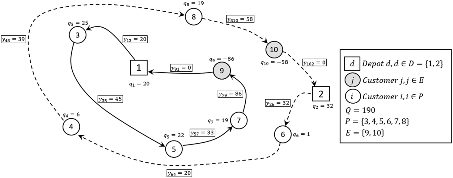
However, it is not possible to obtain the solution presented in Fig. 1 by adapting the formulation reported in Burger et al. (2018). In this optimal solution, Vehicles 1 and 2, starting from Depots 1 and 2, respectively, transfer units at Pickup Location 3. The formulation by Burger et al. (2018) does not allow customers to be visited more than once since it would require multiple and different labels to be assigned to a node due to vehicles from different depots visiting that node, which the formulation does not permit. This is evident if we try to label the nodes in Fig. 1, which will result in assigning two different labels to Customer 3 (that is visited by Vehicle 1 and 2), i.e.
Fig. 1
Optimal solution obtained by adapting the compact formulation presented in Bektaş (2012) and in this paper to the FD-mVRPT.
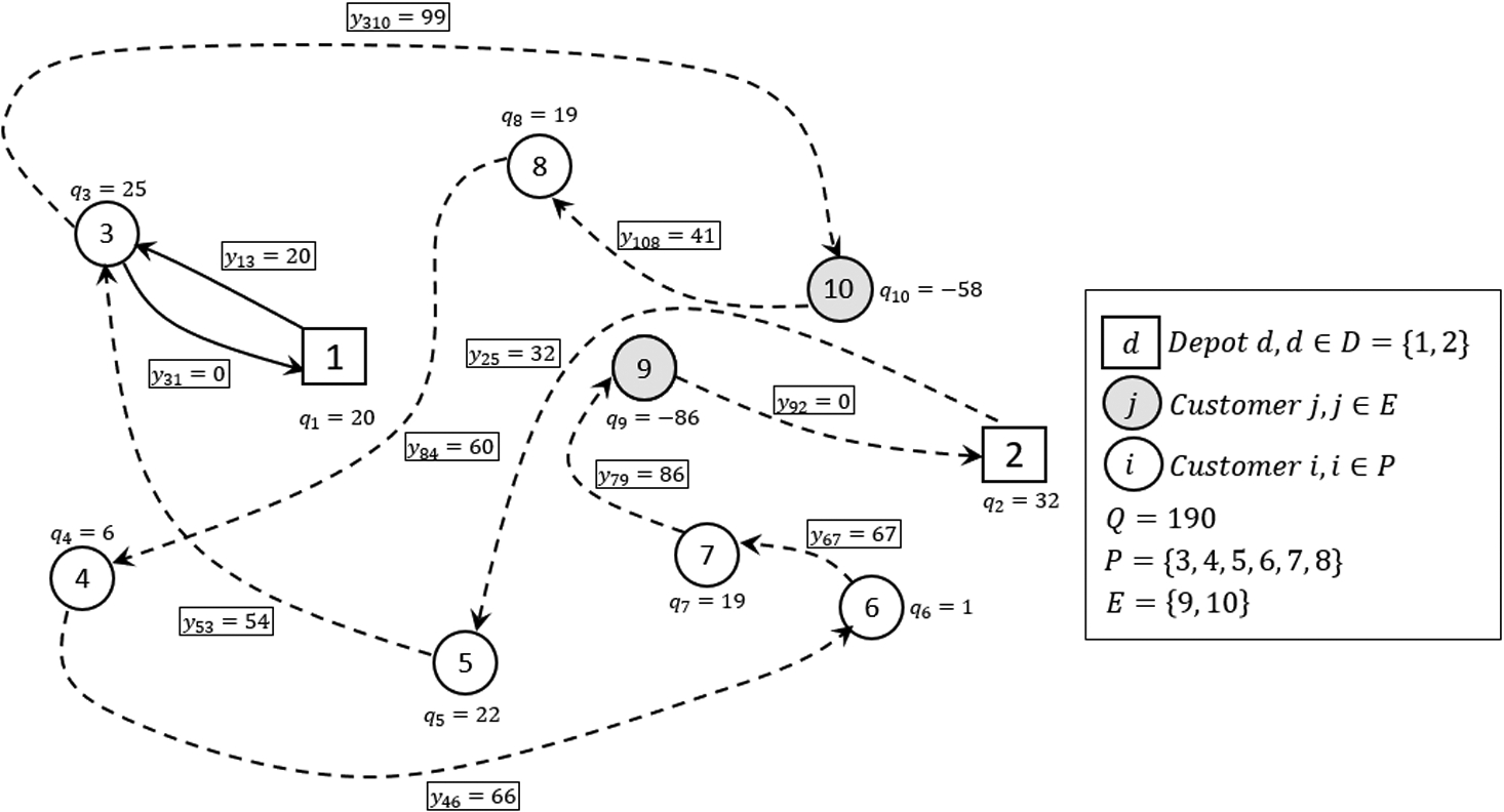
Fig. 2
Optimal solution obtained by adapting the compact formulation presented in Burger et al. (2018) to the FD-mVRPT.
3.1.1General Formulation for the FD-mVRPT
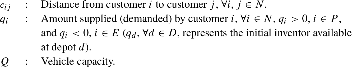
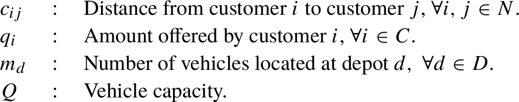
Before we introduce the model, consider the following notation:
Sets and parameters: 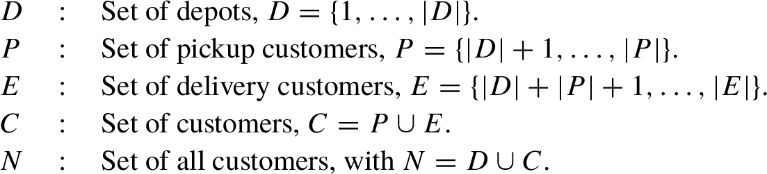 Parameters:
Let
(34)
(35)
(36)
(37)
(38)
(39)
(40)
(41)
(42)
(43)
(44)
The KB-SECs cannot be extended to this problem since they are developed on the assumption that each node is visited exactly once; and thus, can lead to a contradiction on the labels assigned to nodes visited more than once. Therefore, we only extend the GG-SECs, which are presented next.
Letting
(45)
(46)
(47)
(48)
We adapt FDC1s, FDC2s, FDC3s, Constraints (20)–(24), (25)–(27) and (29)–(33), to enforce vehicles to return to their starting points.
3.2FD-mDCPTP
The FD-mDCPTP can be stated as follows. We have a set D of depots with
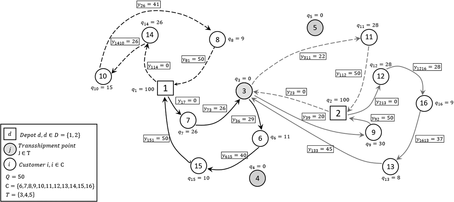
We present an example to illustrate the FD-mDCPTP (see Fig. 3). We have two depots,
Fig. 3
An illustration of the FD-mDCPTP.
3.2.1General Formulation for the FD-mDCPTP
Sets: 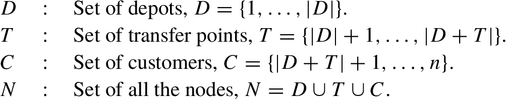 Parameters:
Let
(49)
(50)
(51)
(52)
(53)
(54)
(55)
(56)
(57)
(58)
(59)
(60)
The objective function (49) minimizes the total cost, while Constraints (50) and (51) enforce that each vehicle departs and returns to its depot, respectively. Constraints (52) and (53) ensure that each costumer is visited exactly once, while Constraints (54) are the standard flow conservation constraints. Constraints (55) capture if the transfer location is used, while Constrains (56) enforce that if the transfer location is open (
Letting
(61)
(62)
(63)
(64)
(65)
Constraints (61) prohibit to send products between depots, while Constraints (62) enforce the flow variables
We use FDC1s and FDC3s, Constraints (20)–(24) and (29)–(33), respectively, as fixed-destination constraints. FDC2s will generate restrictive solutions and may not be able to even find a feasible solution. Consequently, we will not investigate the performance of FDC2s in our computational experiments.
4Computational Results
In this section, we compare the results obtained for the proposed two-index formulation with those obtained for the formulations reported in the literature on the FD-mATSP. We also present the results of this compact formulation extended to the FD-mVRPT and the FD-mDCPTP. All formulations were solved directly in OPL using CPLEX version 12.8.0, with default parameters using a computer with an Intel Xeon(R) CPU E5-2623 v4 @2.60GHZx8 with 62.8 GB of RAM. A time limit of 10,800 seconds was set for all runs.
4.1Instances
For the FD-mATSP, we use the first 20 instances presented in Bektaş (2012) and derived from TSPLIB (1997), as displayed in Table 1. The columns of this table denote the instance number (Instance), the ATSP problem from where it was derived (ATSP instance), the number of nodes (n), and the number of depots (
Table 1
Instances for the FD-mATSP used in Bektaş (2012).
| Instance | Name | n | |
| 1 | ftv33.tsp | 34 | 2 |
| 2 | ftv35.tsp | 36 | 2 |
| 3 | ftv38.tsp | 39 | 2 |
| 4 | p43.tsp | 43 | 2 |
| 5 | ftv44.tsp | 45 | 2 |
| 6 | ftv47.tsp | 48 | 2 |
| 7 | ry48p.tsp | 48 | 2 |
| 8 | ft53.tsp | 53 | 2 |
| 9 | ftv55.tsp | 56 | 2 |
| 10 | ftv55.tsp | 56 | 3 |
| 11 | ftv64.tsp | 65 | 2 |
| 12 | ftv64.tsp | 65 | 3 |
| 13 | ft70.tsp | 70 | 2 |
| 14 | ft70.tsp | 70 | 3 |
| 15 | ftv70.tsp | 71 | 2 |
| 16 | ftv70.tsp | 71 | 3 |
| 17 | kro124p.tsp | 100 | 2 |
| 18 | kro124p.tsp | 100 | 3 |
| 19 | ftv170.tsp | 171 | 5 |
| 20 | ftv170.tsp | 171 | 5 |
For the FD-mVRPT, we created two sets of instances. The first set, displayed in Table 2, is based on the instances reported in Table 1 for which sets P and E, as well as the parameters
Step 1: (Generation of temporal customer demands
Step 2: (Generation of P and E). We first determine an integer
Step 3: (Checking Feasibility). Given the partitioned sets P and E, it is possible that the resulting supply is less than the demand. Therefore, we determine F units, such that
Step 4: (Generating vehicle capacity.) We assume a unique vehicle to be present in each depot for both set of instances. We determine the capacity of each vehicle as
Step 5: (Generation of
Table 2
Modified instances derived from the TSPLIB (1997) for FD-mVRPT.
| Instance | Name | n | Q | ||||
| 1 | ftv33.tsp | 34 | 32 | 2 | 16 | 16 | 560 |
| 2 | ftv35.tsp | 36 | 34 | 2 | 18 | 16 | 590 |
| 3 | ftv38.tsp | 39 | 37 | 2 | 18 | 19 | 630 |
| 4 | p43.tsp | 43 | 41 | 2 | 22 | 19 | 720 |
| 5 | ftv44.tsp | 45 | 43 | 2 | 21 | 22 | 760 |
| 6 | ftv47.tsp | 48 | 46 | 2 | 24 | 22 | 780 |
| 7 | ry48p.tsp | 48 | 46 | 2 | 24 | 22 | 730 |
| 8 | ft53.tsp | 53 | 51 | 2 | 24 | 27 | 820 |
| 9 | ftv55.tsp | 56 | 54 | 2 | 28 | 26 | 840 |
| 10 | ftv55.tsp | 56 | 53 | 3 | 26 | 27 | 650 |
| 11 | ftv64.tsp | 65 | 63 | 2 | 33 | 30 | 1070 |
| 12 | ftv64.tsp | 65 | 62 | 3 | 30 | 32 | 650 |
| 13 | ft70.tsp | 70 | 68 | 2 | 34 | 34 | 1190 |
| 14 | ft70.tsp | 70 | 67 | 3 | 33 | 34 | 730 |
| 15 | ftv70.tsp | 71 | 69 | 2 | 34 | 35 | 1200 |
| 16 | ftv70.tsp | 71 | 68 | 3 | 34 | 34 | 750 |
| 17 | kro124p.tsp | 100 | 98 | 2 | 47 | 51 | 1680 |
| 18 | kro124p.tsp | 100 | 97 | 3 | 50 | 47 | 1100 |
| 19 | ftv170.tsp | 171 | 166 | 5 | 86 | 80 | 1040 |
| 20 | ftv170.tsp | 171 | 166 | 5 | 84 | 82 | 1090 |
Table 3
Modified instances derived from the MDVRP (Cordeau, 2007) for FD-mVRPT.
| Instance | Name | n | Q | ||||
| 21 | p01 | 54 | 50 | 4 | 27 | 23 | 100 |
| 22 | p02 | 54 | 50 | 4 | 27 | 23 | 160 |
| 23 | p03 | 80 | 75 | 5 | 42 | 33 | 140 |
| 24 | p04 | 108 | 100 | 8 | 50 | 50 | 370 |
| 25 | p05 | 102 | 100 | 2 | 50 | 50 | 370 |
| 26 | p06 | 103 | 100 | 3 | 50 | 50 | 250 |
| 27 | p07 | 104 | 100 | 4 | 50 | 50 | 190 |
| 28 | p12 | 82 | 80 | 2 | 41 | 39 | 110 |
| 29 | p13 | 82 | 80 | 2 | 41 | 39 | 200 |
| 30 | p14 | 82 | 80 | 2 | 41 | 39 | 180 |
| 31 | pr01 | 52 | 48 | 4 | 83 | 61 | 230 |
| 32 | pr02 | 100 | 96 | 4 | 21 | 23 | 200 |
| 33 | pr03 | 148 | 144 | 4 | 48 | 44 | 195 |
| 34 | pr04 | 196 | 192 | 4 | 96 | 96 | 320 |
| 35 | pr07 | 78 | 72 | 6 | 35 | 37 | 200 |
For the FD-mDCPTP, we created the set of instances displayed in Tables 4 and 5, which are based on those reported in Tables 2 and 3. We generate the number of transfer points using a uniform distribution,
Table 4
Modified instances derived from the TSPLIB (1997) for the FD-mDCPTP.
| Instance | Name | n | Q | |||
| 1 | ftv33.tsp | 34 | 30 | 2 | 2 | 510 |
| 2 | ftv35.tsp | 36 | 31 | 2 | 3 | 530 |
| 3 | ftv38.tsp | 39 | 35 | 2 | 2 | 570 |
| 4 | p43.tsp | 43 | 39 | 2 | 2 | 690 |
| 5 | ftv44.tsp | 45 | 41 | 2 | 2 | 710 |
| 6 | ftv47.tsp | 48 | 44 | 2 | 2 | 780 |
| 7 | ry48p.tsp | 48 | 43 | 2 | 3 | 730 |
| 8 | ft53.tsp | 53 | 49 | 2 | 2 | 820 |
| 9 | ftv55.tsp | 56 | 52 | 2 | 2 | 840 |
| 10 | ftv55.tsp | 56 | 50 | 3 | 3 | 650 |
| 11 | ftv64.tsp | 65 | 61 | 2 | 2 | 1020 |
| 12 | ftv64.tsp | 65 | 59 | 3 | 3 | 620 |
| 13 | ft70.tsp | 70 | 66 | 2 | 2 | 1160 |
| 14 | ft70.tsp | 70 | 65 | 3 | 2 | 710 |
| 15 | ftv70.tsp | 71 | 66 | 2 | 3 | 1120 |
| 16 | ftv70.tsp | 71 | 66 | 3 | 2 | 730 |
| 17 | kro124p.tsp | 100 | 96 | 2 | 2 | 1650 |
| 18 | kro124p.tsp | 100 | 94 | 3 | 3 | 1050 |
| 19 | ftv170.tsp | 171 | 163 | 5 | 3 | 1020 |
| 20 | ftv170.tsp | 171 | 163 | 5 | 3 | 1070 |
Table 5
Modified instances derived from the MDVRP (Cordeau, 2007) for the FD-mDCPTP.
| Instance | Name | n | Q | |||
| 21 | p01 | 54 | 47 | 4 | 3 | 100 |
| 22 | p02 | 54 | 48 | 4 | 2 | 100 |
| 23 | p03 | 80 | 73 | 5 | 2 | 140 |
| 24 | p04 | 108 | 97 | 8 | 3 | 360 |
| 25 | p05 | 102 | 98 | 2 | 2 | 370 |
| 26 | p06 | 103 | 97 | 3 | 3 | 240 |
| 27 | p07 | 104 | 97 | 4 | 3 | 180 |
| 28 | p12 | 82 | 77 | 2 | 3 | 100 |
| 29 | p13 | 82 | 78 | 2 | 2 | 110 |
| 30 | p14 | 82 | 78 | 2 | 2 | 110 |
| 31 | pr01 | 52 | 45 | 4 | 3 | 80 |
| 32 | pr02 | 100 | 94 | 4 | 2 | 160 |
| 33 | pr03 | 148 | 142 | 4 | 2 | 220 |
| 34 | pr04 | 196 | 189 | 4 | 3 | 310 |
| 35 | pr07 | 78 | 69 | 6 | 3 | 80 |
4.2Results for FD-mATSP
We report the results obtained for ALF (proposed formulation), NLF (Burger et al., 2018) and MCF (Bektaş, 2012) developed for the FD-mATSP (see Section 2). These results are displayed in Table 6, where, for each formulation, we report the LP relaxation value (
Based on the results presented above, we can make the following remarks:
1 NLF outperformed the other two compact formulations for the FD-mATSP, whereas ALF outperformed MCF.
2 From an analytical comparison, none of the formulations dominates the other in terms of the strength of their LP relaxations.
3 From the practitioners’ viewpoint, we recommend using the formulations in the order: NLF, ALF and MCF.
Table 6
Results for the ALF, NLF, and MCF-based formulations on the FD-mATSP.
| ALF | NLF (Burger et al., 2018) | MCF (Bektaş, 2012) | ||||||||
| Instance | Name | CPU/Gap | CPU/Gap | CPU/Gap | ||||||
| 1 | ftv33.tsp | 1424.75 | 1579 | 62.39 | 1425.36 | 1579 | 26.79 | 1426.13 | 1579 | 52.69 |
| 2 | ftv35.tsp | 1590.35 | 1669 | 6.12 | 1600.43 | 1669 | 4.39 | 1593.23 | 1669 | 6.07 |
| 3 | ftv38.tsp | 1640.77 | 1730 | 20.48 | 1647.12 | 1730 | 10.51 | 1643.55 | 1730 | 16.41 |
| 4 | p43.tsp | 2092.18 | 5695 | 99.38 | 2092.16 | 5695 | 36.61 | 2092.25 | 5695 | 1565.15 |
| 5 | ftv44.tsp | 1709.92 | 1802 | 12.31 | 1715.66 | 1802 | 4.62 | 1715.24 | 1802 | 13.37 |
| 6 | ftv47.tsp | 1848.25 | 1975 | 30.13 | 1862.57 | 1975 | 27.47 | 1862.73 | 1975 | 53.5 |
| 7 | ry48p.tsp | 15218.09 | 15864 | 47.94 | 15219.05 | 15864 | 36.59 | 15218.09 | 15864 | 109.45 |
| 8 | ft53.tsp | 6733.17 | 7396 | 17.83 | 6715.23 | 7396 | 36.41 | 6793.2 | 7396 | 12.97 |
| 9 | ftv55.tsp | 1642.58 | 1797 | 204.65 | 1647.44 | 1797 | 147.66 | 1550.73 | 1797 | 531.34 |
| 10 | ftv55tsp | 1865.66 | 2013 | 81.03 | 1869.5 | 2013 | 9.06 | 1879.31 | 2013 | 380.31 |
| 11 | ftv64.tsp | 1889.29 | 1992 | 104.5 | 1896.4 | 1992 | 40.96 | 1899.13 | 1992 | 150.38 |
| 12 | ftv64.tsp | 1928.62 | 2062 | 78.95 | 1924.88 | 2062 | 365.66 | 1961.76 | 2062 | 1297.76 |
| 13 | ft70.tsp | 40788.65 | 41105 | 224.95 | 40803.28 | 41105 | 35.76 | 40803.52 | 41105 | 373.86 |
| 14 | ft70.tsp | 41726.99 | 42272 | 664.24 | 41759.79 | 42272 | 471.79 | 41731.58 | 42272 | 1016.82 |
| 15 | ftv70.tsp | 1968.26 | 2074 | 76.74 | 1980.55 | 2074 | 41.56 | 1982.31 | 2074 | 197.39 |
| 16 | ftv.70.tsp | 2099.75 | 2296 | 2600.35 | 2102.01 | 2296 | 778.26 | 2114.43 | 2295.99 | 6180.85 |
| 17 | fro124p.tsp | 36329.11 | 37407 | 245.53 | 36329.11 | 37407 | 144.62 | 36329.11 | 37407 | 659.36 |
| 18 | kro124p.tsp | 36874.41 | 38076 | 252.7 | 36774.28 | 38076 | 169.92 | 36792.4 | 38076 | 1144.4 |
| 19 | ftv170.tsp | 3121.47 | 4087 | 20.13% | 3122.63 | 3920 | 16.26% | 3134.22 | 26751 | 88.14% |
| 20 | ftv170.tsp | 2093.78 | 5696.99 | 42.61% | 3095.11 | 3833.999 | 14.39% | 3107.31 | 26596 | 88.15% |
4.3Results for FD-mVRPT
We report the results obtained by the proposed formulation (ALF) and the one by Bektaş (2012) (MCF) adapted for the FD-mVRPT presented in Section 3.1.1. Recall that the formulation based on NLF (Burger et al., 2018) is only an approximation and does not represent the problem exactly. The results are displayed in Table 7. The columns in this table are identical to those in Table 6, and the sign “–” is used to denote an infeasible solution generated by a formulation. ALF obtained the minimum T/Gap in 33 out of 35 cases, outperforming MCF. The average optimality gaps attained for ALF and MCF are 4.72% and 7.12% with average computational times of 5555.8 and 6275.5, respectively.
From the results presented above, we can infer the following:
1 The proposed formulation (ALF) outperformed (MCF) for the FD-mVRPT.
2 From the practitioners’ viewpoint, our proposed formulation is effective in modelling logistics problems having fixed-destinations in which customers can be visited more than once as in FD-mVRPT.
4.4Results for FD-mDCPTP
In Table 8, we present the results obtained by the proposed formulation (ALF) versus the one reported in Bektaş (2012) (MCF) for the FD-mDCPTP (see Section 3.2). The columns in this table are identical to those in Table 6. ALF outperformed MCF in 29 out of 35 cases. The average optimality gap for the former and the latter are 11.17% and 18.76%, respectively, with a maximum gap of 46.51% for the former and 92.31% for the latter. The proposed two-index formulation is therefore more suitable for modelling variations of the fixed-destination routing problems in which transfer locations are used to minimize transportation costs.
Table 7
Results for FD-mVRPT.
| ALF | MCF | ||||||
| Instance | Name | CPU/Gap | CPU/Gap | ||||
| 1 | ftv33.tsp | 909.63 | 1401 | 20.16 | 899.47 | 1401 | 43.93 |
| 2 | ftv35.tsp | 1006.67 | 1560 | 19.63 | 1006.63 | 1560 | 45.74 |
| 3 | ftv38.tsp | 1045.32 | 1623 | 36.22 | 1045.24 | 1623 | 79.52 |
| 4 | p43.tsp | 2612.14 | 5630 | 181.22 | 2612.14 | 5630 | 127.07 |
| 5 | ftv44.tsp | 1114.05 | 1710 | 75.48 | 1114.05 | 1710 | 95.59 |
| 6 | ftv47.tsp | 1194.56 | 1834 | 45.32 | 1194.56 | 1834 | 70.69 |
| 7 | ry48p.tsp | 9229.94 | 15049 | 234.5 | 9229.94 | 15049 | 162.4 |
| 8 | ft53.tsp | 4411.48 | 7103 | 101.13 | 4407.62 | 7103 | 178.45 |
| 9 | ftv55.tsp | 1146.70 | 1666 | 88.18 | 1145.27 | 1666 | 202.99 |
| 10 | ftv55tsp | 1240.06 | 1713 | 80.98 | 1229.19 | 1713 | 292.06 |
| 11 | ftv64.tsp | 1272.95 | 1905 | 145.71 | 1269.72 | 1905 | 284.33 |
| 12 | ftv64.tsp | 1332.10 | 1932 | 197.17 | 1322.52 | 1932 | 645.91 |
| 13 | ft70.tsp | 23483.95 | 39924 | 0.13% | 23469.02 | 40124 | 1.12% |
| 14 | ft70.tsp | 24869.02 | 40293 | 0.68% | 23869.02 | 40752 | 2.74% |
| 15 | ftv70.tsp | 1255.34 | 1995 | 247.54 | 1254.21 | 1995 | 481.88 |
| 16 | ftv.70.tsp | 1384.61 | 2058 | 354.41 | 1384.61 | 2058 | 1218.66 |
| 17 | fro124p.tsp | 23255.89 | 37280 | 6618.4 | 23255.89 | 37905 | 4.17% |
| 18 | kro124p.tsp | 23418.21 | 37444 | 1.79% | 23418.21 | 38375 | 4.84% |
| 19 | ftv170.tsp | 2319.22 | 3376 | 16.29% | 2319.22 | 7674 | 67.32% |
| 20 | ftv170.tsp | 2300.82 | 3742 | 25.16% | 2300.82 | – † | 10800 |
| 21 | p01 | 271.34 | 449 | 1697.67 | 278.97 | 449 | 3057.51 |
| 22 | p02 | 263.11 | 445 | 573.872 | 263.11 | 445 | 1354.55 |
| 23 | p03 | 340.18 | 558 | 1.51% | 340.28 | 561 | 2.63% |
| 24 | p04 | 338.96 | 641 | 6.91% | 348.20 | 644 | 9.55% |
| 25 | p05 | 335.15 | 623 | 3.20% | 343.37 | 642 | 11.40% |
| 26 | p06 | 342.23 | 649 | 5.82% | 357.92 | 644 | 6.63% |
| 27 | p07 | 347.45 | 676 | 9.21% | 371.079 | 923 | 40.38% |
| 28 | p12 | 817.43 | 1616 | 9.65% | 1100.66 | 1642 | 11.21% |
| 29 | p13 | 925.21 | 1617 | 9.74% | 1100.66 | 1626 | 10.35% |
| 30 | p14 | 817.43 | 1617 | 9.74% | 1100.66 | 1626 | 10.40% |
| 31 | pr01 | 510.19 | 867 | 102.17 | 510.19 | 867 | 725.11 |
| 32 | pr02 | 546.88 | 1174 | 2.61% | 546.88 | 1239 | 10.6% |
| 33 | pr03 | 762.99 | 1821 | 21.01% | 823.77 | 2054 | 37.7% |
| 34 | pr04 | 998.14 | 2288 | 40.16% | 1018.13 | – † | 10800 |
| 35 | pr07 | 625.90 | 1074 | 1.44% | 625.90 | 1100 | 5.80% |
† Infeasible solution.
Table 8
Results for the FD-mDCPTP.
| ALF | MCF | ||||||
| Instance | Name | CPU/Gap | CPU/Gap | ||||
| 1 | ftv33.tsp | 1368.13 | 1595 | 167.96 | 1368.62 | 1595 | 822.57 |
| 2 | ftv35.tsp | 1519.53 | 1690 | 85.63 | 1519.72 | 1690 | 162.11 |
| 3 | ftv38.tsp | 1556.56 | 1760 | 740.09 | 1556.56 | 1760 | 1170.64 |
| 4 | p43.tsp | 2883.29 | 5728 | 0.15% | 2883.29 | 5728 | 0.10% |
| 5 | ftv44.tsp | 1713.88 | 1869 | 336.69 | 1713.88 | 1869 | 737.34 |
| 6 | ftv47.tsp | 1794.81 | 2084 | 8.21% | 1811.23 | 2134 | 6.43% |
| 7 | ry48p.tsp | 14497.04 | 16967 | 2.96% | 14497.04 | 16919 | 4.27% |
| 8 | ft53.tsp | 6788.11 | 7812 | 2.16% | 6849.43 | 7812 | 7730.61 |
| 9 | ftv55.tsp | 1599.02 | 1870 | 3.68% | 1619.74 | 1863 | 2.15% |
| 10 | ftv55tsp | 1828.73 | 2085 | 1577.87 | 1849.92 | 2085 | 1932.86 |
| 11 | ftv64.tsp | 1912.83 | 2090 | 3.26% | 1914.87 | 2117 | 4.28% |
| 12 | ftv64.tsp | 2042.2 | 2558 | 10.14% | 2055.966 | 2600 | 14.91% |
| 13 | ft70.tsp | 39886.53 | 40924 | 0.20% | 39886.9 | 41328 | 2.53% |
| 14 | ft70.tsp | 40989.59 | 45312 | 4.87% | 40993.4 | 44616 | 6.69% |
| 15 | ftv70.tsp | 1960.52 | 2246 | 1.84% | 1962.43 | 2243 | 4.24% |
| 16 | ftv.70.tsp | 2192.5 | 2652 | 8.93% | 2194.64 | 2514 | 5.43% |
| 17 | fro124p.tsp | 35875.4 | 51698 | 11.32% | 35875.4 | 48613 | 23.11% |
| 18 | kro124p.tsp | 37538.71 | 58555 | 24.77% | 37561.039 | 58324 | 32.87% |
| 19 | ftv170.tsp | 3549.63 | 7452 | 36.15% | 3551.57 | 6277 | 42.25% |
| 20 | ftv170.tsp | 3579.12 | 7229 | 40.42% | 3580.48 | 47485 | 92.31% |
| 21 | p01 | 416.68 | 514 | 7.63% | 416.68 | 532 | 11.80% |
| 22 | p02 | 427.10 | 524 | 8.88% | 427.10 | 540 | 12.38% |
| 23 | p03 | 532.53 | 667 | 12.64% | 532.53 | 928 | 37.64% |
| 24 | p04 | 581.51 | 638 | 2.28% | 581.51 | 748 | 17.05% |
| 25 | p05 | 574.00 | 667 | 7.40% | 574.00 | 672 | 8.31% |
| 26 | p06 | 587.22 | 732 | 14.51% | 587.22 | 867 | 27.93% |
| 27 | p07 | 606.61 | 819 | 21.31% | 606.64 | 977 | 34.59% |
| 28 | p12 | 968.16 | 1229 | 1.71% | 968.16 | 1314 | 10.43% |
| 29 | p13 | 973.42 | 1222 | 0.93% | 973.42 | 1222 | 1.20% |
| 30 | p14 | 973.42 | 1222 | 1.76% | 973.42 | 1222 | 1.21% |
| 31 | pr01 | 846.45 | 1059 | 8.36% | 846.45 | 1105 | 12.05% |
| 32 | pr02 | 1048.51 | 1563 | 23.14% | 1048.51 | 2736 | 56.43% |
| 33 | pr03 | 1346.24 | 2784 | 44.48% | 1346.24 | 3848 | 60.21% |
| 34 | pr04 | 1366.37 | 3041 | 46.51% | 1366.37 | 4861 | 66.78% |
| 35 | pr07 | 1016.39 | 1679 | 31.73% | 1016.39 | 2588 | 57.04% |
5Concluding Remarks
We have presented a compact formulation for the fixed-destination multi-depot asymmetric travelling salesman problem (FD-mATSP), wherein m salesmen depart from D depots and return to their origins after collectively visiting a set of customers exactly once. The proposed compact formulation labels an arc based on the depot from where the salesman visits that arc. This label is used as a flow that is maintained throughout the tour of a salesman from that depot. We show that the proposed and existing formulations for the FD-mATSP do not dominate each other in terms of the strength of their linear programming relaxations. The proposed formulation was demonstrated to be more versatile and effective to solve other variations of this problem. We have demonstrated this by applying it to the solution of two important extensions of the FD-mATSP, namely, the fixed-destination multiple vehicle routing problems with transshipment (FD-mVRPT), and the fixed-destination multi-depot collection problem with transfer points (FD-mDCPTP). The proposed formulation outperformed a three-index formulation due to Bektaş (2012) and a two-index formulation due to Burger et al. (2018) when adapted to both problems. Hence, the proposed compact formulation has the potential to effectively solve various routing and logistics problems with applicability in contemporary logistics and manufacturing management environments. For future work, we propose to extend the proposed formulation to other routing problems as well as design more effective exact algorithms based on a polyhedral analysis of the model that exploits the underlying flow-based structure.
References
1 | Aguayo, M.M. (2016). Modeling, Analysis, and Exact Algorithms for Some Biomass Logistics Supply Chain Design and Routing Problems. PhD thesis, Virginia Polytechnic Institute and State University. |
2 | Anily, S., Hassin, R. ((1992) ). The swapping problem. Networks, 22: (4), 419–433. |
3 | Bektaş, T. ((2012) ). Formulations and Benders decomposition algorithms for multidepot salesmen problems with load balancing. European Journal of Operational Research, 216: (1), 83–93. |
4 | Bektaş, T., Gouveia, L., Santos, D. ((2020) ). Compact formulations for multi-depot routing problems: theoretical and computational comparisons. Computers & Operations Research, 124: , 105084. |
5 | Burger, M. ((2014) ). Exact and compact formulation of the fixed-destination travelling salesman problem by cycle imposement through node currents. In: Huisman, L.I.W.A.D. (Ed.), Operations Research Proceedings 2013. Springer, Cham. |
6 | Burger, M., Su, Z., Schutter, B.D. ((2018) ). A node current-based 2-index formulation for the fixed-destination multi-depot travelling salesman problem. European Journal of Operational Research, 265: (2), 463–477. |
7 | Chira, C., Sedano, J., Villar, J.R., Cámara, M., Corchado, E. ((2014) ). Urban bicycles renting systems: Modelling and optimization using nature-inspired search methods. Neurocomputing, 135: , 98–106. |
8 | Cordeau (2007). Multiple Depot VRP Instances. http://neo.lcc.uma.es/vrp/vrp-instances/multiple-depot-vrp-instances/. |
9 | Davendra, D. ((2010) ). Traveling Salesman Problem: Theory and Applications. BoD–Books on Demand. |
10 | Gavish, B., Graves, S.C. (1978). The travelling salesman problem and related problems. Working paper GR-078-78. Cambridge, MA: Operation Research Center, Massachusetts Institute of Technology. |
11 | Golden, B.L., Raghavan, S., Wasil, E.A. ((2008) ). The Vehicle Routing Problem: Latest Advances and New Challenges. Springer, New York. |
12 | Guastaroba, G., Speranza, M.G., Vigo, D. ((2016) ). Intermediate facilities in freight transportation planning: a survey. Transportation Science, 50: (3), 763–789. |
13 | Kara, I., Bektaş, T. ((2006) ). Integer linear programming formulations of multiple salesman problems and its variations. European Journal of Operational Research, 174: (3), 1449–1458. |
14 | Kumar, S.N., Panneerselvam, R. ((2012) ). A survey on the vehicle routing problem and its variants. Intelligent Information Management, 4: (03), 66. |
15 | Laporte, G. ((1992) a). The traveling salesman problem: an overview of exact and approximate algorithms. European Journal of Operational Research, 59: (2), 231–247. |
16 | Laporte, G. ((1992) b). The vehicle routing problem: an overview of exact and approximate algorithms. European Journal of Operational Research, 59: (3), 345–358. |
17 | Lawler, E.L., Lenstra, J.K., Rinnooy Kan, A.H., Shmoys, D.B. (1985). The traveling salesman problem; a guided tour of combinatorial optimization. Journal of the Operational Research Society. |
18 | Lou, Z., Li, Z., Luo, L., Dai, X. ((2016) ). Study on multi-depot collaborative transportation problem of milk-run pattern. In: MATEC Web of Conferences, Vol. 81: , 01004. EDP Sciences. |
19 | Malik, W., Rathinam, S., Darbha, S. ((2007) ). An approximation algorithm for a symmetric generalized multiple depot, multiple travelling salesman problem. Operations Research Letters, 35: (6), 747–753. |
20 | Montoya-Torres, J.R., Franco, J.L., Isaza, S.N., Jiménez, H.F., Herazo-Padilla, N. ((2015) ). A literature review on the vehicle routing problem with multiple depots. Computers & Industrial Engineering, 79: , 115–129. |
21 | Paredes-Belmar, G., Lüer-Villagra, A., Marianov, V., Cortés, C.E., Bronfman, A. ((2017) ). The milk collection problem with blending and collection points. Computers and Electronics in Agriculture, 134: , 109–123. |
22 | Ramos, T.R.P., Gomes, M.I., Póvoa, A.P.B. ((2020) ). Multi-depot vehicle routing problem: a comparative study of alternative formulations. International Journal of Logistics Research and Applications, 23: (2), 103–120. |
23 | Reinelt, G. ((1994) ). The Traveling Salesman: Computational Solutions for TSP Applications. Springer-Verlag, Berlin. |
24 | Toth, P., Vigo, D. ((2002) ). The Vehicle Routing Problem. SIAM, Philadelphia. |
25 | TSPLIB (1997). A Library of traveling salesmen and related problem instances. http://elib.zib.de/pub/mp-testdata/tsp/tsplib/atsp/index.html. |
26 | Zhang, R., Yun, W.Y., Moon, I. ((2009) ). A reactive tabu search algorithm for the multi-depot container truck transportation problem. Transportation Research Part E: Logistics and Transportation Review, 45: (6), 904–914. |


