
2D PET Image Reconstruction Using Robust L1 Estimation of the Gaussian Mixture Model
Abstract
An image or volume of interest in positron emission tomography (PET) is reconstructed from gamma rays emitted from a radioactive tracer, which are then captured and used to estimate the tracer’s location. The image or volume of interest is reconstructed by estimating the pixel or voxel values on a grid determined by the scanner. Such an approach is usually associated with limited resolution of the reconstruction, high computational complexity due to slow convergence and noisy results.
This paper presents a novel method of PET image reconstruction using the underlying assumption that the originals of interest can be modelled using Gaussian mixture models. Parameters are estimated from one-dimensional projections using an iterative algorithm resembling the expectation-maximization algorithm. This presents a complex computational problem which is resolved by a novel approach that utilizes
1Introduction
In positron emission tomography (PET), image reconstruction implies generating an image of a radiotracer’s concentration to estimate physiologic parameters for objects (volumes) of interest. Pairs of photons arise from emissions of annihilated positrons, and crystals placed in the scanner detect these pairs. When two are activated at the same time, the device records an event. Each possible pair of crystals is connected by a line or volume of response (LOR, VOR), depending on whether the scan is 2D or 3D. Assuming there are no contaminating physical effects or noise, the total number of coincidence events detected and the total amount of tracer contained in the tube are proportional. In the 2D case, we observe events along lines of response (LORs) joining two detector elements, lying within a specified imaging plane. The data are recorded as event histograms (sinograms or projected data) or as a list of recorded photon-pair events (list-mode data). Classic PET image reconstruction methodology is explained in more detail in e.g. Tong et al. (2010), Alessio and Kinahan (2006) or Reader and Zaidi (2007).
Modern image reconstruction methods are mostly based on maximum-likelihood expectation-maximization (MLEM) iterations. Maximum likelihood is used as the optimization criterion, combined with the expectation-maximization algorithm for finding its solution. To overcome the computational complexity and slow convergence of the MLEM, the ordered subsets expectation-maximization (OSEM) algorithm has been introduced (Hudson and Larkin, 1994). Since MLEM or OSEM estimation of pixels or voxels is usually noisy (Tong et al., 2010), use of post-filtering methods is necessary. On the one hand, image reconstruction from its projections is a mature research field with well known methods and proven results. On the other hand, known limitations made a challenge for a different approach presented in this paper.
In image segmentation, a number of algorithms based on model-based techniques utilizing prior knowledge have been proposed to model uncertainty, cf. Zhang et al. (2001, 1994). The Gaussian mixture model (GMM) is well-known and widely used in a variety of segmentation and classification problems (Friedman and Russell, 1997; Ralašić et al., 2018), as many observed quantities exhibit behaviour congruent with the model. A good overview of the application of GMMs and their generalizations to problems in image classification, image annotation and image retrieval can be found, e.g. in Tian (2018). However, in those problems the sample is from the GMM itself, whereas in this case the observed data is lower-dimensional (i.e. lines) and the points of origin are unknown.
In this paper, we propose a new robust method for reconstructing an object from a simulated PET image. The challenge of estimating Gaussian parameters from lower-dimensional data is solved by utilizing a novel
2Two-Dimensional PET Imaging
Fig. 1
(a) Simulated measurements for
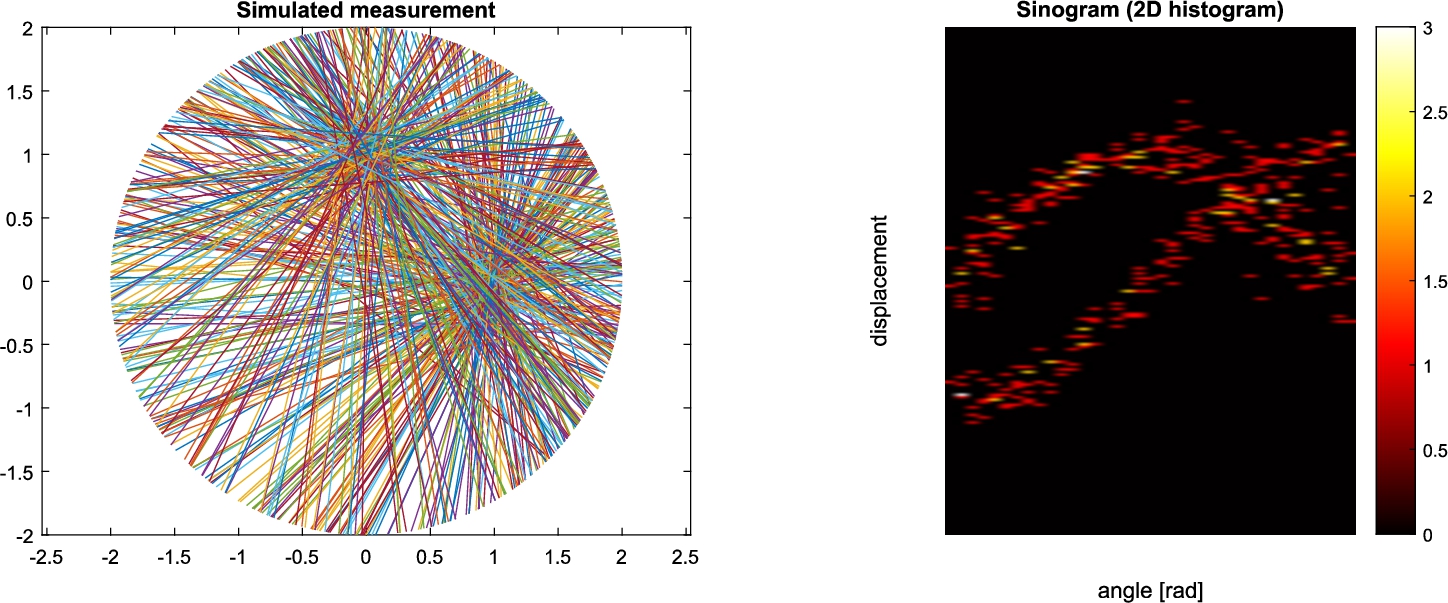
Data are collected along lines lying within a specific imaging plane. Traditionally, data are organized into sets of projections, integrals along all lines (LORs) for a fixed direction ϕ. The collection of all projections for
3Estimating the Gaussian Mixture Model
A Gaussian mixture model (Reynolds, 2015) is a weighted sum of K component Gaussian densities as given by the equation:
(1)
(2)
Traditionally in this setting, the GMMs are used to model activity concentration in voxels (Layer et al., 2015) or pixel values (Nguyen and Wu, 2013). Those models do not take into account the spatial correlation between observations, which can be corrected by introducing Markov random fields (Layer et al., 2015; Nguyen and Wu, 2013). In other image segmentation problems, this can be addressed by modelling the mixture weights as probability vectors, thereby creating a spatially varying finite mixture model (SVFMM) (Xiong and Huang, 2015).
Here, we apply the GMM directly to the spatial data, focusing only on the locations and not the values at those locations. In other words, the location of the tracer, i.e. the particles that originate the gamma rays, is represented by the the K Gaussian components. The points
As mentioned earlier, Gaussian mixture models have naturally appeared in many signal processing (Yu and Sapiro, 2011; Léger et al., 2011) and biometrics problems (Reynolds, 2015; Reynolds et al., 2000). Due to the flexibility of the mixtures, GMMs are convenient and effective for modelling various types of signals, as well as image inverse and missing/noisy data problems.
Note that in our simulations we assume that K, the number of mixture components, is known. In practical applications it should also be estimated, which is a further (and not insignificant) problem. For mixture components that are sufficiently separated in space, such as in Fig. 1, the sinogram itself could give insight into the most adequate number of components, otherwise ideas suggested in, e.g. Leroux (1992), Chen (1995), Cheng (2005), should be explored.
For clarity, in this section we focus only on one Gaussian component. Assuming we know a set of N events whose points of origin come from a Gaussian distribution with parameters
3.1Estimation of μ Using Minimal Distance
Each event in two dimensions is uniquely given by its slope
(3)
In general, the squared distance between d-dimensional vectors is defined as
(4)
First, note that for a fixed
(5)
(6)
1)
where2)
3)
4)
(7)
3.2Estimation of Σ Using 1D Projections
In the two-dimensional setting, since Σ is a symmetric matrix,
Figure 2 depicts a single event and its corresponding LOR. Recall that the line is determined by two parameters, one of which is the slope
(8)
Fig. 2
Illustration of the rotation. The event (LOR) is parallel to the new y-axis.
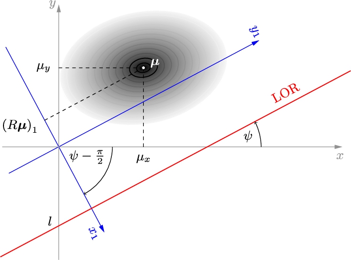
Given the original event parameters, the coordinates of the intersection of the event and the new x-axis are
(9)
We can use these one-dimensional projections and their squared (Euclidian) distance from the mean, to estimate the variance in (9). This squared distance is equal to
(10)
(11)
(12)
4EM-Like Algorithm
In many statistical models, maximum likelihood parameter estimation can not be performed directly since most equations do not have an explicit closed solution. Several iterative methods have been developed to combat this, most notably the expectation-maximization (EM) algorithm. It had been proposed and used in many different circumstances before its proper introduction in Dempster et al. (1977). The name comes from its two-step setup, namely the expectation (E) and maximization (M) step which interchange until an acceptable solution is found. In the context of GMMs, and generally in emission tomography (Shepp and Vardi, 1982), the issue is that the true mixture membership is unknown (latent). The E step for given mixture parameters estimates probabilities
1. Compute class membership probabilities. For each event, compute the squared distance from each component mean. We distinguish between a hard classification where we assign the event to its nearest component, and a soft classification where membership probability is inversely proportional to the squared distance.
2. Estimate component parameters. Either from a hard or soft classification, where each event participates with its proportional share, parameters of each component are estimated using methodology from Section 3.
This approach allows for different variants, depending on the type of distance used (Tafro and Seršić, 2019).
In this paper, initial steps of the iterative algorithm use Euclidian distance in (4). Since later iterations improve the estimates, the distance gradually transforms into the Mahalanobis distance, i.e.
(13)
5Results
To evaluate the methodology, we experimented in the two-dimensional setting with
First, for proof of concept we show that the method in Section 3 provides good estimates with both
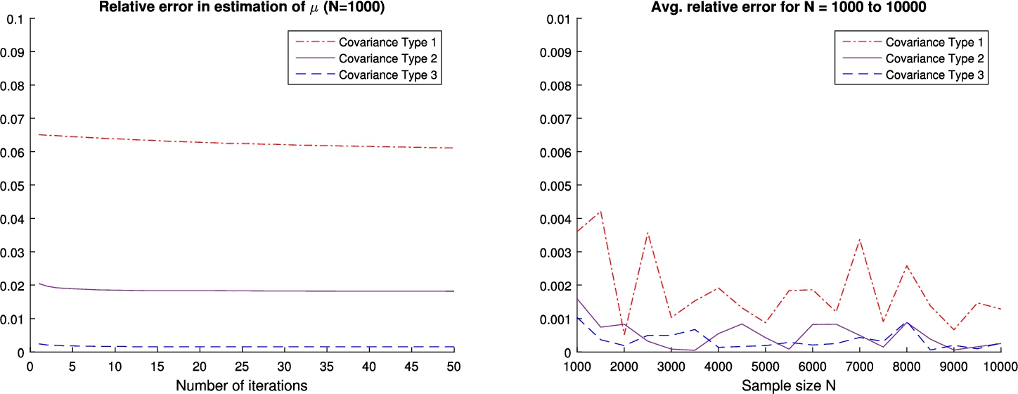
Fig. 3
Left: Relative error in estimation of
5.1One-Dimensional Estimation
Accuracy of an estimate
Initial value of α in the distance weight matrix was set to zero, and proportionally increased to 1 in the final iteration. The left side of Fig. 3 illustrates how the errors in the estimation of
For each of these types of covariances we then simulated a measurement from
Table 1
Mean estimation error,
| 13.78% | 11.88% | 9.28% | |
| 8.27% | 7.61% | 7.6% |
| 4.28% | 3.66% | 2.93% | |
| 2.61% | 2.38% | 2.37% |
Given that the variance of the traditional standard deviation estimator (from points) equals
5.2Two-Dimensional Estimation
For
For synthetic measurements from a variety of original (real) GMMs the algorithm proved robust regardless of the values of initial parameters, with estimation using
Table 2 shows the percentage of correctly classified events for several combinations of covariance matrices, where a total of
Table 2
Correct classification,
| Cov. 1 | Cov. 2 | Comp. 1 | Comp. 2 | Total |
| 87.63% | 93.49% | 89.83% | ||
| 93.52% | 92.13% | 93.00% | ||
| 91.26% | 95.83% | 92.98% |
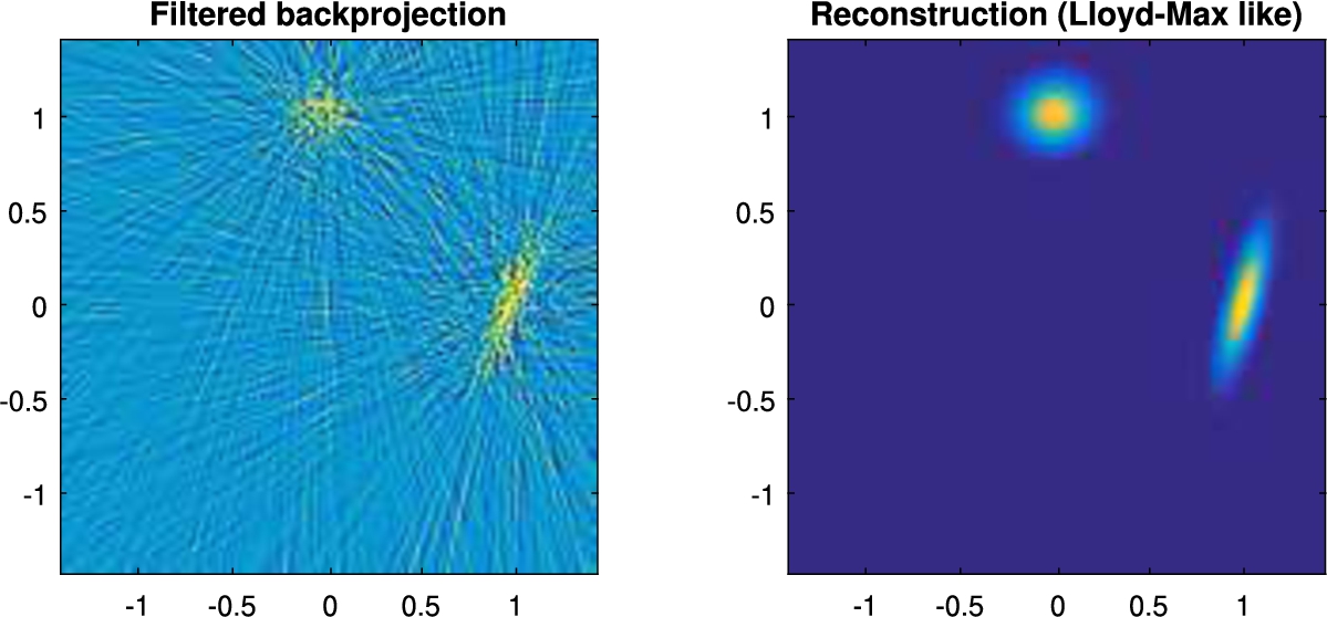
An illustration of the results for
Fig. 4
(a) Classical FBP reconstruction. (b) Proposed reconstruction using
6Conclusion
These results show proof of concept that it is possible to reconstruct data from latent mixture models using lower-dimensional observations and state-of-the-art computational techniques. Estimation from lower-dimensional measurements had not been thoroughly developed for Gaussian mixture models in general, and especially in this context. This paper shows that the main obstacle, slow computational speed, can be evaded by an alternative approach to minimization, which opens the door to various new procedures. Further work includes other metrics and membership calculation and utilizing traditional methods to obtain the number of mixing components and optimal initial values.
The fact that the reconstructed image is given by its parametric model (mean vectors
Appendices
Appendix
The
(14)
We insert it into all other equations and get a new system with only two unknown parameters:
(15)
We insert
(16)
Parameter
The value of parameter
(17)
Return to a higher dimension is achieved by putting calculated parameter value
Acknowledgments
This research has been supported by the Croatian Science Foundation under the project IP-2019-04-6703.
References
1 | Alessio, A., Kinahan, P. ((2006) ). PET image reconstruction. Nuclear Medicine, 1: , 1–22. https://doi.org/10.1118/1.2358198. |
2 | Bektaş, S., Şişman, Y. ((2010) ). The comparison of L11 and L22-norm minimization methods. International Journal of Physical Sciences, 5: (11), 1721–1727. |
3 | Chen, J. ((1995) ). Optimal rate of convergence for finite mixture models. The Annals of Statistics, 23: (1), 221–233. https://doi.org/10.1214/aos/1176324464. |
4 | Cheng, Y.-m. ((2005) ). Maximum weighted likelihood via rival penalized EM for density mixture clustering with automatic model selection. IEEE Transactions on Knowledge and Data Engineering, 17: (6), 750–761. https://doi.org/10.1109/TKDE.2005.97. |
5 | Dempster, A.P., Laird, N.M., Rubin, D.B. ((1977) ). Maximum likelihood from incomplete data via the EM algorithm. Journal of the Royal Statistical Society. Series B, 39: , 1–38. https://doi.org/10.2307/2984875. |
6 | Friedman, N., Russell, S. ((1997) ). Image segmentation in video sequences: a probabilistic approach. In: Proceedings of the Thirteenth Conference on Uncertainty in Artificial Intelligence, UAI’97, pp. 175–181. http://dl.acm.org/citation.cfm?id=2074226.2074247. |
7 | Golub, G.H., Van Loan, C.F. ((2012) ). Matrix Computations, Vol. 3: . JHU Press. https://doi.org/10.1137/1028073. |
8 | Helgason, S. ((1999) ). The Radon Transform, Vol. 2: . Springer. |
9 | Hudson, H.M., Larkin, R.S. ((1994) ). Accelerated image reconstruction using ordered subsets of projection data. IEEE Transactions on Medical Imaging, 13: (4), 601–609. https://doi.org/10.1109/42.363108. |
10 | Layer, T., Blaickner, M., Knäusl, B., Georg, D., Neuwirth, J., Baum, R.P., Schuchardt, C., Wiessalla, S., Matz, G. ((2015) ). PET image segmentation using a Gaussian mixture model and Markov random fields. EJNMMI Physics, 2: (1), 9. https://doi.org/10.1186/s40658-015-0110-7. |
11 | Léger, F., Yu, G., Sapiro, G. ((2011) ). Efficient matrix completion with Gaussian models. In: 2011 IEEE International Conference on Acoustics, Speech and Signal Processing (ICASSP). IEEE, pp. 1113–1116. |
12 | Leroux, B.G. (1992). Consistent estimation of a mixing distribution. The Annals of Statistics, 1350–1360. https://doi.org/10.1214/aos/1176348772. |
13 | Lloyd, S. ((1982) ). Least squares quantization in PCM. IEEE Transactions on Information Theory, 28: (2), 129–137. https://doi.org/10.1109/TIT.1982.1056489. |
14 | Natterer, F. ((1986) ). The Mathematics of Computerized Tomography, Vol. 32: . Siam. https://doi.org/10.1137/1.9780898719284. |
15 | Nguyen, T.M., Wu, Q.J. ((2013) ). Fast and robust spatially constrained Gaussian mixture model for image segmentation. IEEE Transactions on Circuits and Systems for Video Technology, 23: (4), 621–635. https://doi.org/10.1109/TCSVT.2012.2211176. |
16 | O’Sullivan, F., Pawitan, Y. ((1993) ). Multidimensional density estimation by tomography. Journal of the Royal Statistical Society: Series B (Methodological), 55: (2), 509–521. https://doi.org/10.1111/j.2517-6161.1993.tb01919.x. |
17 | Ralašić, I., Seršić, D., Petrinović, D. ((2019) ). Off-the-shelf measurement setup for compressive imaging. IEEE Transactions on Instrumentation and Measurement, 68: (2), 502–511. https://doi.org/10.1109/TIM.2018.2847018. |
18 | Ralašić, I., Tafro, A., Seršić, D. ((2018) ). Statistical compressive sensing for efficient signal reconstruction and classification. In: 2018 4th International Conference on Frontiers of Signal Processing (ICFSP), pp. 44–49. https://doi.org/10.1109/ICFSP.2018.8552059. |
19 | Rani, M., Dhok, S., Deshmukh, R. ((2018) ). A systematic review of compressive sensing: concepts, implementations and applications. IEEE Access, 6: , 4875–4894. https://doi.org/10.1109/ACCESS.2018.2793851. |
20 | Reader, A.J., Zaidi, H. ((2007) ). Advances in PET image reconstruction. PET Clinics, 2: (2), 173–190. PET Instrumentation and Quantification. https://doi.org/10.1016/j.cpet.2007.08.001. |
21 | Reynolds, D. ((2015) ). Gaussian mixture models. In: Li, S.Z., Jain, A.K. (Eds.), Encyclopedia of Biometrics. Springer, Boston, MA. https://doi.org/10.1007/978-1-4899-7488-4_196. |
22 | Reynolds, D.A., Quatieri, T.F., Dunn, R.B. ((2000) ). Speaker verification using adapted Gaussian mixture models. Digital Signal Processing, 10: (1–3), 19–41. https://doi.org/10.1006/dspr.1999.0361. |
23 | Rousseeuw, P.J., Croux, C. ((1993) ). Alternatives to the median absolute deviation. Journal of the American Statistical association, 88: (424), 1273–1283. https://doi.org/10.1080/01621459.1993.10476408. |
24 | Shepp, L.A., Vardi, Y. ((1982) ). Maximum likelihood reconstruction for emission tomography. IEEE Transactions on Medical Imaging, 1: (2), 113–122. https://doi.org/10.1109/TMI.1982.4307558. |
25 | Sović Kržić, A., Seršić, D. ((2018) ). L1 minimization using recursive reduction of dimensionality. Signal Processing, 151: , 119–129. https://doi.org/10.1016/j.sigpro.2018.05.002. |
26 | Tafro, A., Seršić, D. ((2019) ). Iterative algorithms for Gaussian mixture model estimation in 2D PET Imaging. In: 2019 11th International Symposium on Image and Signal Processing and Analysis (ISPA), pp. 93–98. https://doi.org/10.1109/ISPA.2019.8868570. |
27 | Tian, D. ((2018) ). Gaussian mixture model and its applications in semantic image analysis. Journal of Information Hiding and Multimedia Signal Processing, 9: (3), 703–715. |
28 | Tong, S., Alessio, A.M., Kinahan, P.E. ((2010) ). Image reconstruction for PET/CT scanners: past achievements and future challenges. Imaging in Medicine, 2.5: , 529–545. https://doi.org/10.2217/iim.10.49. |
29 | Xiong, T., Huang, Y. ((2015) ). Robust Gaussian mixture modelling based on spatially constraints for image segmentation. Journal of Information Hiding and Multimedia Signal Processing, 6: (5), 857–868. |
30 | Yu, G., Sapiro, G. ((2011) ). Statistical compressed sensing of Gaussian mixture models. IEEE Transactions on Signal Processing, 59: (12), 5842–5858. https://doi.org/10.1109/TSP.2011.2168521. |
31 | Zhang, J., Modestino, J.W., Langan, D.A. ((1994) ). Maximum-likelihood parameter estimation for unsupervised stochastic model-based image segmentation. IEEE Transactions on Image Processing, 3: (4), 404–420. https://doi.org/10.1109/83.298395. |
32 | Zhang, Y., Brady, M., Smith, S. ((2001) ). Segmentation of brain MR images through a hidden Markov random field model and the expectation-maximization algorithm. IEEE Transactions on Medical Imaging, 20: (1), 45–57. https://doi.org/10.1109/42.906424. |


