
Randentropy: A Software to Measure Inequality in Random Systems
Abstract
The software Randentropy is designed to estimate inequality in a random system where several individuals interact moving among many communities and producing dependent random quantities of an attribute. The overall inequality is assessed by computing the Random Theil’s Entropy. Firstly, the software estimates a piecewise homogeneous Markov chain by identifying the change-points and the relative transition probability matrices. Secondly, it estimates the multivariate distribution function of the attribute using a copula function approach and finally, through a Monte Carlo algorithm, evaluates the expected value of the Random Theil’s Entropy. Possible applications are discussed as related to the fields of finance and human mobility.
1Introduction
The issue of measuring inequality in a system found extensive treatment in the literature. One interesting approach is based on entropic measures. Starting from the pioneering work by Shannon (1948) on the mathematical theory of communication, the concept of entropy has found a rapid development and diffusion in many scientific communities. Notable examples are statistics (see, e.g. Kullback and Leibler, 1951), statistical mechanics (see, e.g. Jaynes, 1957), economy (see, e.g. Theil, 1967) and ecology (see, e.g. Phillips et al., 2006), just to name a few.
Recent efforts have been dedicated mainly to introduce new entropies as the cumulative residual entropy (see, Rao et al., 2004) or the cumulative past entropy (see, Di Crescenzo and Longobardi, 2009). In the meantime, and mainly motivated by economic problems, the notion of random entropy has emerged in terms of a normalization of a random process. The random entropy shares the same functional form as the classical entropy but is related to a random process (D’Amico and Di Biase, 2010). This more general entropy was called by the author Dynamic Theil Entropy. Nevertheless, we refer to it as Random Entropy, to avoid any possible misunderstanding with other dynamic entropies which are expressed as deterministic functions as in Di Crescenzo and Longobardi (2002), Asadi and Zohrevand (2007) and Calì et al. (2020).
The Random Entropy allows to quantify uncertainty in a random system evolving in time and encompasses recent approaches and measures introduced in Curiel and Bishop (2016). In this paper, we consider the general model considered in a previous work (D’Amico et al., 2019) and we present a software that permits the calculation of the inequality in a general system composed by a number of interacting individuals. Any individual moves among several communities in time and according to its membership, and depending on that of the other individuals, produces an attribute. The dynamic of individuals among the communities is described according to a piecewise homogeneous Markov chain which requires the identification of an unknown number of change-points (i.e. where the Markov chain changes its dynamic). Conditional on the occupancy of the communities, the individuals produce an attribute in quantities expressed by a multivariate probability distribution where the dependence structure is managed by a copula function. Finally, using a Monte Carlo algorithm, we show how to compute the moments of the Random Entropy.
The main innovation brought by this research is the building of the software Randentropy. It contemplates different aspects that were only partially considered in other research papers. Indeed, different studies deal with software and packages related to multi-state models of Markovian type. For example, in Ferguson et al. (2012) the authors consider a package for computing marginal and conditional occupation probabilities for Markov and non-Markov multi-state models, including the censoring problem and the use of covariates. In Jackson et al. (2011), multi-state models for panel data observed continuously and generally based on the Markov assumption have been instead considered. The possibility to obtain a time-varying model is considered using piecewise-constant time-dependent covariates. Contrarily to these studies, our software gives different transition probability matrices according to the change-point detection methodology presented in Polansky (2007), which is based only on observations of the Markov process and not on additional covariates. Moreover, once the piecewise homogeneous Markov chain is identified, the software provides sequences of dependent random vectors denoting the ownership of an attribute by the individuals of the system. Thus, the system becomes a multivariate Markov reward process on which the Random Entropy is evaluated. To our knowledge, our software is the only one that computes the Random Entropy and does it in a very general framework that encompasses recent contributions presenting diversity measurement based on (deterministic) entropy where the migration of individuals among the communities is not allowed, see Marcon and Hérault (2015a). Of potential interest is also the use of the software Randentropy to problems approached with the traditional concept of entropy, see e.g. Behrendt et al. (2019) and Saad and Ruai (2019).
The subsequent sections of this paper present the general mathematical model, relevant scenarios of application and the software main characteristics, both the CLI (Command Line Interface) and GUI (Graphical User Interface) are described.
2Theory
The main function driving the development of the software we are presenting here (i.e. Randentropy) refers to the computation of a measure of inequality on the distribution of a given attribute among a set of N individuals. The quantity of this attribute depends on a discriminatory criterion, according to whom the individual belongs to a given group. Accordingly to the nomenclature mainly derived within the ecology community, but preserving its general validity also in other domains, we denote the set of individuals as a meta-community that is partitioned in several interacting groups called communities. This description is the same adopted in Marcon and Hérault (2015b).
Let denote the meta-community by
The sequence of the visited communities by any individual
Firstly, we assume an independence assumption between the dynamics of the individuals. Thus, the community process for every individual will be denoted simply by
Moreover, we assume that
The symbols
Intuitively, the term piecewise refers to the existence of some points in time where the dynamic changes consistently. These times are called change-points. They break up the timeline into several sub-periods within whom the Markov process is homogeneous.
Fig. 1
Example of three change-points.
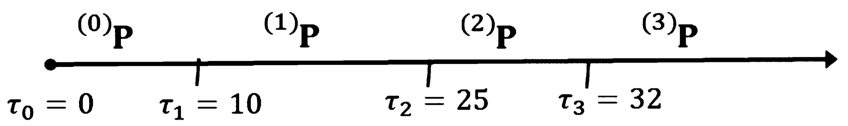
However, for the sake of clarity of presentation, consider the example illustrated in Fig. 1 where three change-points are considered at times
Next step concerns the specification of the processes describing the personal attributes, i.e.
This strategy is pursued first by assuming that the marginal distributions of the attributes of the individuals allocated in the same community at a given time share the same probability distribution function. Formally, let
Before presenting our second main assumption we need to present the concept of copula which will be a key issue in the model and software.
An N-dimensional copula C is any function
Additionally, a dependence structure is introduced through the application of a copula function. This is formally done advancing the second main assumption stating that: the conditional joint distribution of
A notable example of copula function is the Normal (or Gaussian) copula. Let R be a correlation matrix and denote by
In general, the corresponding density of the copula is
Here, the parameters are represented by the correlation matrix R.
As we are interested in measuring the inequality of the distribution of attributes in the meta-community, we need to introduce a measure of inequality. In particular, the measure of inequality we consider allows the user to face with stochastic processes. The measure is based on the Theil entropy (see Theil, 1967), closely related to the Shannon entropy (see Shannon, 1948). Given a probability distribution
(1)
The definition of Theil index has been extended for stochastic processes by D’Amico and Di Biase (2010) and successively applied and further investigated in D’Amico et al. (2012) and in D’Amico et al. (2014) for an additive decomposition of this index. The random extension of the Theil index is, indeed, introduced.
Let
We denote the Random Entropy in the meta-community by the stochastic process
(2)
An explicit formula for the expected value of
The whole computational procedure is made of several steps, thus, to simplify the readability of the reported pseudocode (see Algorithm 1), we are omitting some of the preliminary tasks, such as: the identification of the number K and dislocation in time of the change points
Algorithm 1
Monte Carlo Simulation of the Random Entropy
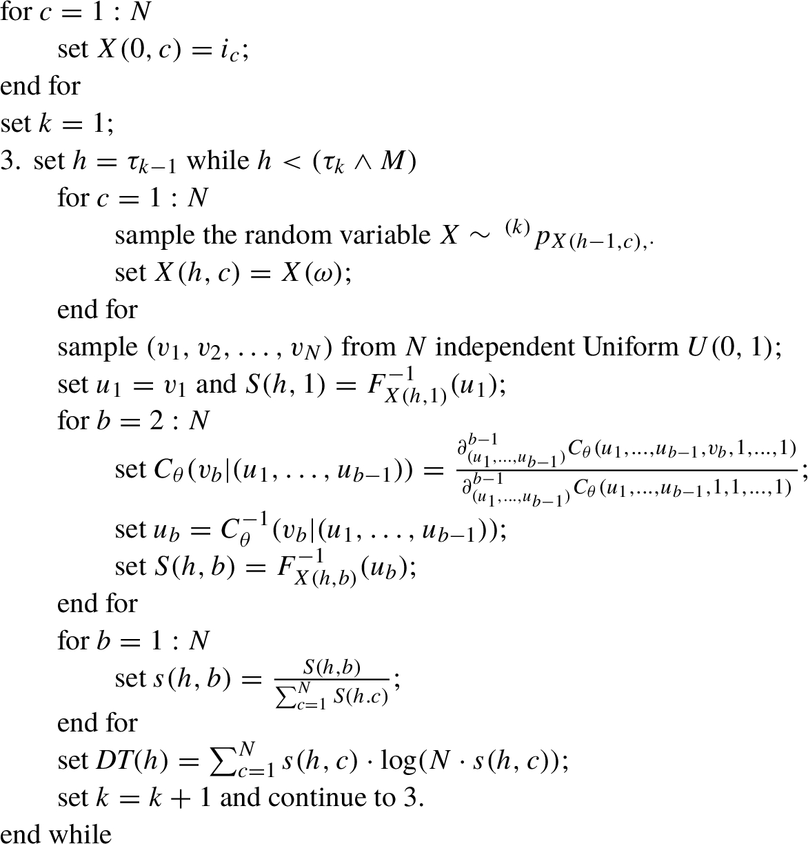
For easiness of notation we adopt the following vectorial notation along the Algorithm 1:
•
•
•
• M denotes the horizon time of the simulation.
The Algorithm 1 generates a vector of observations
The result of Algorithm 1 is a sequence of values
3Relevant Scenarios of Application
In this section we provide a short description of two possible domains of application of the model. Certainly, a variety of additional situations falls well within the described theoretical setting.
3.1Financial Inequality in an Economic Area
This application was originally considered by D’Amico et al. (2018a) and (2018b) and successively in a more comprehensive way in D’Amico et al. (2019). In this framework we have a meta-community that coincides with a given set of countries all belonging to a given Economic Area. A possible case is represented by the European Economic Area. Practically, every country receives a note about its financial creditworthiness, which is expressed in terms of a sovereign credit rating, see e.g. Trueck and Rachev (2009) and D’Amico et al. (2017). Credit ratings are measured in an ordinal scale and assigned by the rating agencies. Moody’s, Standard & Poor’s and Fitch are three major among others.
Each rating class can be seen as a community, in which the countries are allocated at every time. According to its own riskiness (expressed by rating class), each country pays interest rates on its debt. When the interest rates are compared to a benchmark they define the so-called credit spreads. Thus, credit spreads can be seen as personal attributes held by each country in time.
Empirical analysis has shown that credit spreads of European countries are positively correlated, with the exception of Denmark, Sweden and the United Kingdom. To model this complex correlation structure a copula function can be used according to our framework. Once the credit spreads are obtained, it is possible to compute the vector of attributes at time t,
3.2Human Mobility and Environmental Implications
Another area in which the
For example, it would be possible to consider pollution as a variable depending on the specific location, and to measure by the index
4Computational Details and Applications
The software we are presenting here has been engineered so that the main computational kernel is included in a single python module named randentropymod (Storchi, 2020). The cited module contains two classes: randentropykernel and changepoint. The two classes are devoted to the Markov reward approach computation, and to the change-point estimation, respectively. The full software bundle is then composed by two Command Line Interfaces (CLIs): randentropy.py and randentropy_qt.py, and a single Graphical User Interface (GUI) based on PyQt5 Summerfield (2007) (i.e. the Python binding of the cross-platform GUI toolkit).
While the two mentioned CLIs have been specifically developed to perform separately the Markov reward computation (i.e. randentropy.py) and the change-point estimation (i.e. changepoint.py), the GUI has a wider ability. Indeed, the GUI may be used to perform both the change-point estimation as well as the Markov reward computation, and clearly also to easily visualize and explore the obtained results.
The full software suite has been developed within the Linux OS environment. However, once the needed packages are downloaded and installed, it should work, without restrictions, also under Mac OS and Windows thanks to the intrinsic portability nature of the Python programming language. The Python packages, in addition to the aforementioned PyQT5, strictly needed to run the code are: Numpy (see Dubois et al., 1996) and Scipy (Jones et al., 2001) used to engineered the numerical tasks, matplotlib for the plots and data visualization (see Hunter, 2007).
4.1The Randentropykernel Class and Related CLI
As already stated, the randentropykernel class is devoted to the computation of the Random Entropy which is based on the Markov model with dependent rewards as described in Section 2. The class is made of several methods as the one to specify the community matrix (i.e. set_community) and the attributes matrix (i.e. set_attributes), which correspond to the matrices
The randentropy.py is the CLI that is naturally bonded to the mentioned class. As can be seen from Fig. 2, the user has the possibility to specify two input matrices (i.e. to specify both their locations and names): the first one representing the community matrix, while the second is the Attributes one. The mentioned matrices may be stored both on a MatLab file or on a CSV style one.
Fig. 2
CLI for the Markov reward approach.
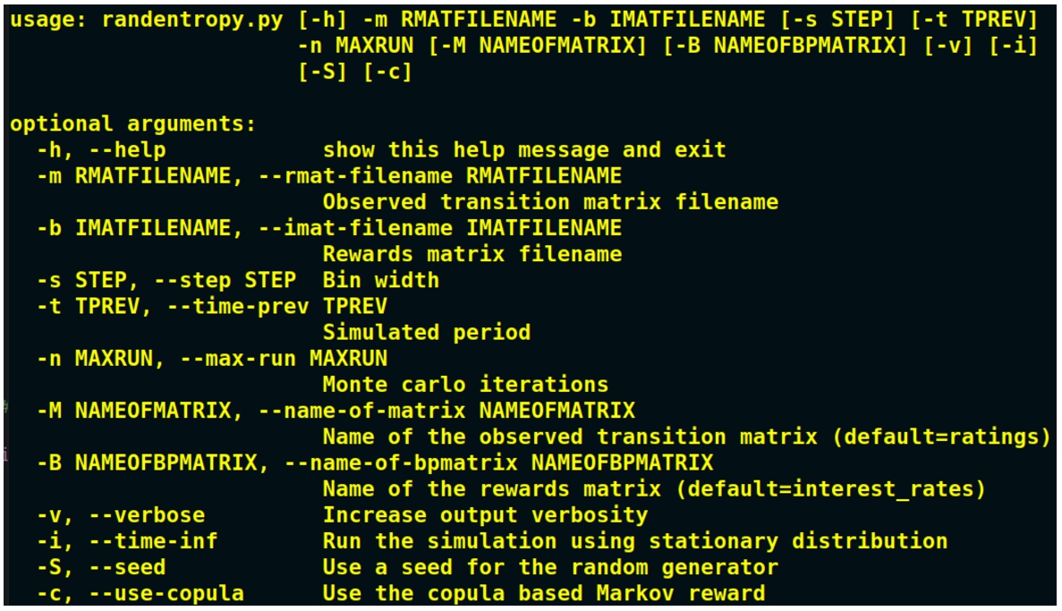
Evidently, the CLI options reported in Fig. 2 reflect the cited randentropykernel capabilities. Then, -s allows for the bin width specification, needed to estimate the probability distribution of the attribute given the community membership. Secondly, -t enables the user to specify the simulated period, and -n refers to the number of Monte Carlo iterations. Optionally, the -i flag allows the user to run the simulation after computing the stationary distribution.
It is finally somehow interesting to report here that: in case one wants to perform the simulation using the stationary distribution π of the Markov chain
4.2The Changepoint Class and Related CLI
As already stated within the randentropymod module there is also the changepoint class. The cited class, and thus the related CLI, is devoted to detect the position of k change-points, where
The most relevant methods within the class are needed to specify the transition matrix (i.e. set_community) and the number of change-points to be detected (i.e. set_num_of_cps). Once the initial settings have been specified, the main computation starts using the compute_cps method. Finally, the calculated x change-points can be retrieved using the get_cp1_found, get_cp2_found and get_cp3_found, respectively, for the first, second and third change-point.
Fig. 3
CLI for change-point detection algorithm.
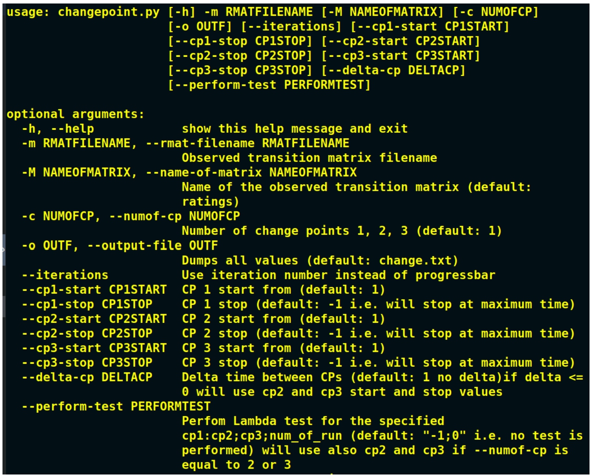
Once again the CLI options, reported in Fig. 3, as expected, reflect the class capabilities. Thus, to run the code, the input transition matrix has to be specified, in terms of a Matlab or a CSV filename, as well as the matrix name within the file (options -m and -M, respectively). The number of change-points to be considered has to be defined as well (i.e. using the -c option), otherwise the code will run assuming a single change-point. Optionally, an output filename, where all the results are written, can be specified using the -o/–output-file option.
Finally, we introduced some methods, and clearly the relative CLI options that can be used also to distribute the computational burden among several processes, thus CPUs. Indeed, while working with a huge amount of data it can be convenient to specify a range of time within which the algorithm is carried out, or to use a specific time distance between two change-points. Thus, the user has the ability to define a range of time for the first change-point (the same applies for the others) via the set_cp1_start_stop method. Similarly, using the set_delta_cp method, one can specify the delta time to be considered among the change-points.
4.3Graphical User Interface
All the previously illustrated functionalities have been integrated also on a GUI (Graphical User Interface). The GUI has been implemented using PyQT5, a comprehensive set of Python bindings for Qt v5 (PyQT, 2012). While we implemented two different CLIs, to fully cover the various aspects implemented within the randentropymod, the GUI is unique and can be access via the randentropy_qt.py file (Storchi, 2020).
Fig. 4
Dialog to specify the input matrices.
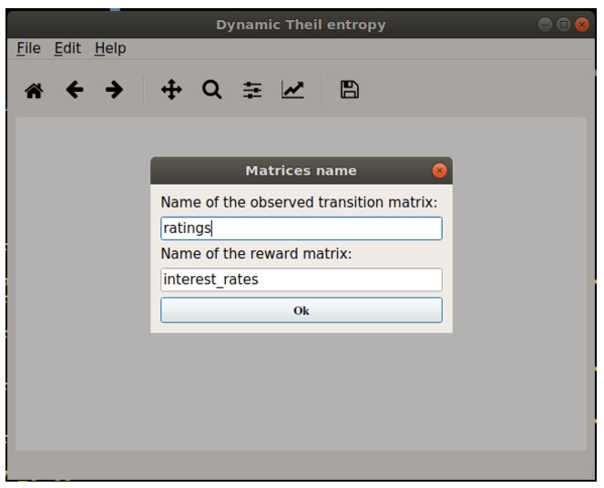
Fig. 5
Dialog to specify the the input parameters related to the Monte Carlo simulation.
The computation starts after choosing an input file, it can be both a Matlab, as well as a CSV, containing two matrices. The first matrix has to contain the data of the variable which is supposed to evolve according to a Homogeneous Markov Chain (HMC) (e.g. in the financial application the variable consists on the sovereign credit ratings, see Section 3.1). As a matter of fact, the first matrix is expected to be named “ratings” by default (see Fig. 4). The second matrix has to refer to the reward process describing the attribute which is driven by the HMC. In the case of the financial application, as illustrated in Section 3.1, this is the credit spread. As the code directly computes the credit spread starting from the interest rates, the second matrix directly collects the interest rate data. Indeed, by default, this matrix within the file is expected to be named “interest_rates” (see Fig. 4).
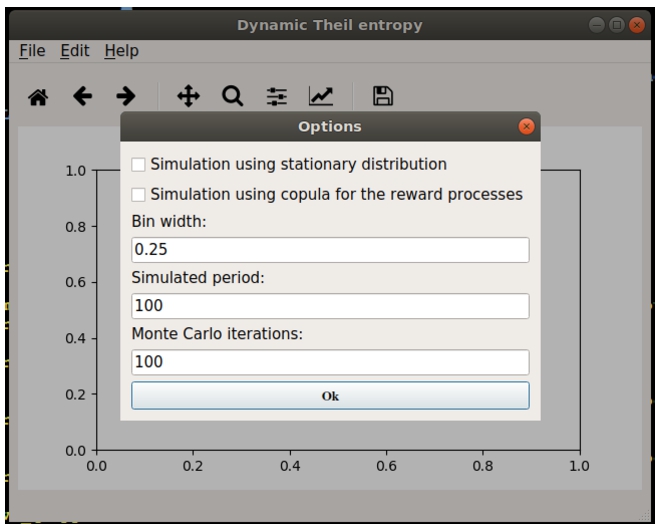
Once the two matrices have been specified, the user may start the computation: Edit -> Run. The use is prompted with a dialog window, reported in Fig. 5, where there is the ability to specify: the bin width to estimate the empirical distributions (one for each ordered variable of the first matrix), the simulated period and the number of Monte Carlo iterations.
Alternatively, the user can flag “Simulation using stationary distribution” to compute the asymptotic values of the Random Theil’s Entropy. After clicking the button OK, the program will start the computation, and when it finishes, it returns the plot of the Dynamic inequality (Fig. 6) that the user has the ability to interact with and to save as a graphical file (i.e. PNG, PDF, PS, and more).
Fig. 6
Output: dynamic inequality.
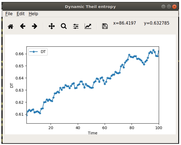
Fig. 7
Histogram of the CS empirical distribution/transition probability matrix.
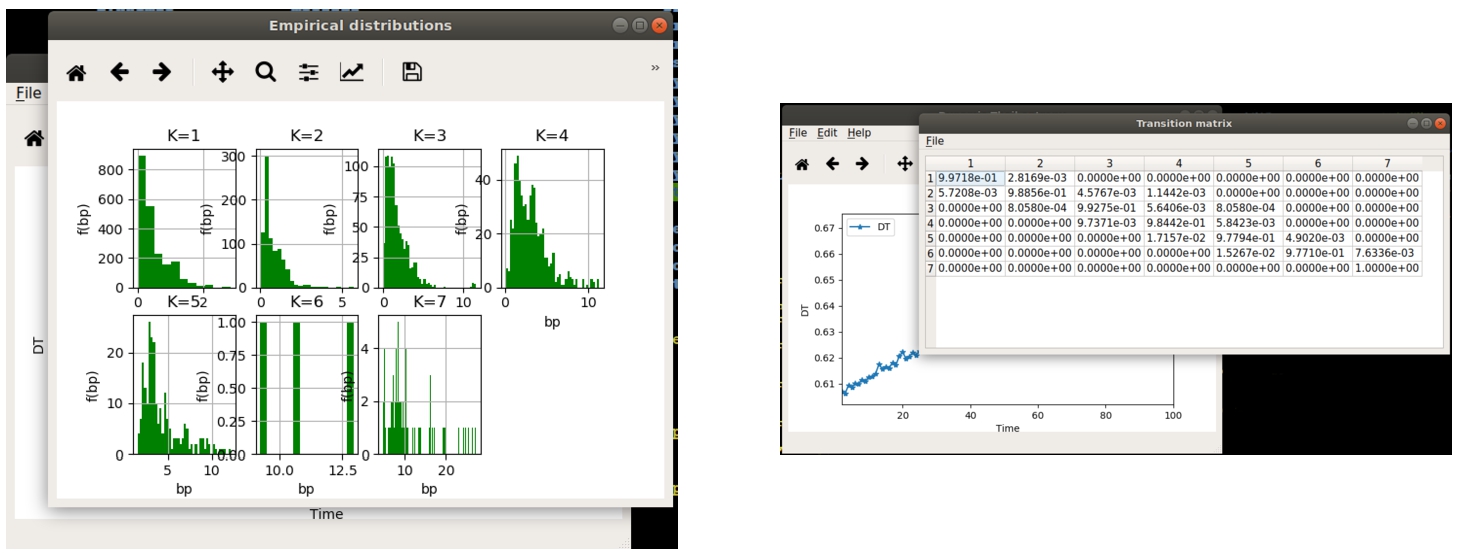
Fig. 8
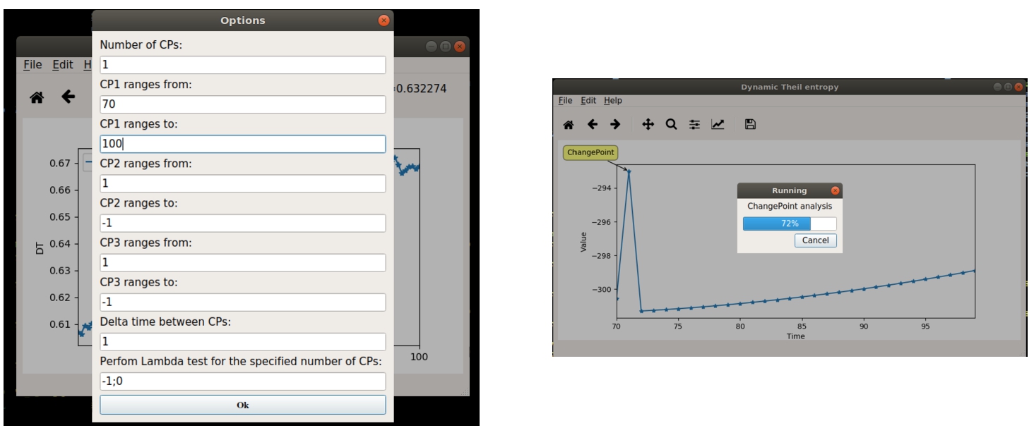
Options required for change-point detection.
Subsequently, by clicking on Edit -> Plot CS distributions the user can plot the histograms of the empirical distributions of the attribute. Moreover, by clicking on Edit –> View Transition matrix the transition probability matrix, estimated on the sequences of visited communities, is shown (Fig. 7).
Finally, with Edit -> RunChangePoint one can run the change-point detection algorithm. As described for the CLI, the code runs after the specification of: the number of change-points to be detected and the corresponding Λ test (see Fig. 8); the range of time where the algorithm is carried out and, eventually, the distance between two subsequent change-points.
In the case reported in Fig. 8, a single change-point is detected within a range of time spreading between
Fig. 9
Output of the change-point detection algorithm.
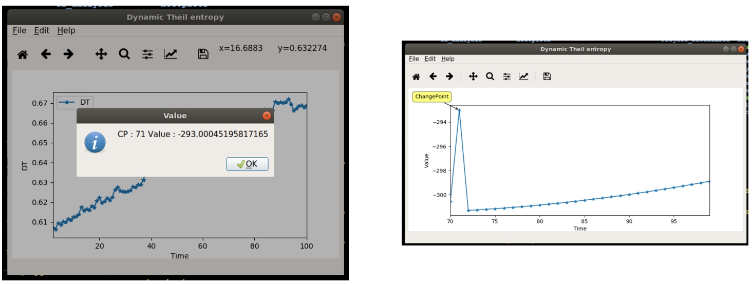
After confirming the chosen options, the computation starts and the GUI returns the plot of the likelihood function estimated on the community data (see in Fig. 9), together with the value of the maximum likelihood function, and the corresponding position of the calculated change-point. Evidently, also in this case, the resulting plot can be saved into a standard graphical file format.
4.4Testing Financial Inequality in an Economic Area
Finally, we will show how the described CLIs and GUI can be used to predict the financial inequality in the European Economic Area according to the theoretical model proposed in D’Amico et al. (2018a, 2018b). In this specific case, the meta-community coincides with all the countries within the European Community. Thus, each rating class, as assigned by rating agencies, can be seen as a community, in which the countries are allocated at every time step. Clearly, as also already stated in the previous section, the credit spread represents the personal attributes held by each country.
The results we are here reporting have been obtained using the monthly rating, attributed by the Standard & Poor’s agency, to the 26 European countries (UK and Cyprus have been excluded in the current meta-community sample) from January 1998 to December 2016 (see, D’Amico et al., 2018a, for extra details on the data-set we are here considering).
To detect the position of a change-point, within the considered horizon time, we compute the maximum value of the likelihood function considered as a function of the position of the change point. Finally, we fix the change point as the value that maximizes the likelihood function. In the proposed software one can use both the changepoint.py CLI as well as the GUI:
Fig. 10
GUI results for the change-point detection, see text for details.
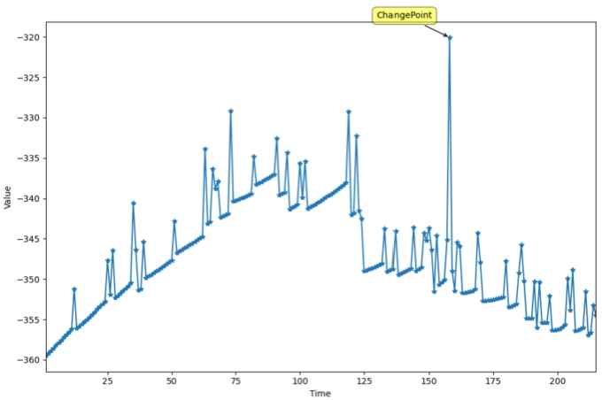
The result is reported in Fig. 10, where the likelihood function is computed depending on the position of the change point (measured on the X-axis). The software detects a change-point at time 158 (the maximum value of the likelihood function). The value 158 corresponds to a change point detected in January 2012. Indeed, at the beginning of 2012 the value of the total credit spread in Europe had a peak of about 10.000 basis points (bp) and this growth was driven by the rise of the securities yield of Greece (2.924 bp), Ireland (1.245 bp) and Portugal (1.385 bp), see D’Amico et al. (2018b) for more detail about the evolution of financial variables. Similarly, for the interested reader, financial examples with multiple change-points can be found in D’Amico et al. (2019)
It is relevant to notice that the software (i.e. the changepoint.py CLI) also provides an indication related to the choice of the best model as it computes the Bayesian information criterion (BIC) to balance the improvement in the goodness of fit test obtained by increasing the number of the parameters obtained by an increase in the number of change points. Precisely, the BIC is evaluated according to the relation
Equivalently, a user can forecast the financial inequality in an economic area and its evolution in time via the randentropy.py (or the GUI):
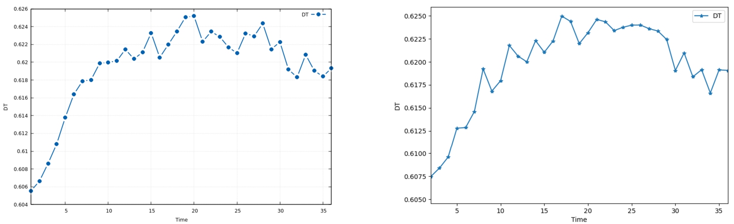
Fig. 11
Random Entropy. Results obtained using the CLI are reported on the left panel, while the ones obtained using the GUI have been reported on the right panel.
As a final remark, it is somehow important to underline that, evidently, a user has the capability of building its own code, to perform the same or similar computations just described, accessing directly the functionalities implemented within the randentropymod Python 3.x module.
5Conclusions and Perspectives
The Randentropy software allows estimating the inequality in a stochastic system according to the framework based on Random Entropy as developed in D’Amico et al. (2019). The methodology is able to consider dependent behaviours of the individuals and time-varying dynamics, which may be of interest in several applied domains. Possible developments of the research include the possibility to consider semi-Markov models, as done in the SemiMarkov R Package developed by Król and Saint-Pierre (2015), to which a reward scheme based on a copula function should be attached, followed by the evaluation of the Random Entropy according to our software.
Random Entropy evaluation, in the presented general framework, is a new and challenging subject of research and is not available in any software; this renders our investigation an “unicum” in the literature of inequality assessment in stochastic systems.
References
1 | Asadi, M., Zohrevand, Y. ((2007) ). On the dynamic cumulative residual entropy. Journal of Statistical Planning and Inference, 137: (6), 1931–1941. |
2 | Behrendt, S., Dimpfl, T., Peter, F.J., Zimmermann, D.J. ((2019) ). RTransferEntropy—quantifying information flow between different time series using effective transfer entropy. SoftwareX, 10: , 100265. |
3 | Calì, C., Longobardi, M., Navarro, J. ((2020) ). Properties for generalized cumulative past measures of information. Probability in the Engineering and Informational Sciences, 34: (1), 92–111. |
4 | Curiel, R.P., Bishop, S. ((2016) ). A measure of the concentration of rare events. Scientific Reports, 6: , 32369. |
5 | D’Amico, G., Di Biase, G. ((2010) ). Generalized concentration/inequality indices of economic systems evolving in time. Wseas Transactions on Mathematics, 9: (2), 140–149. |
6 | D’Amico, G., Di Biase, G., Manca, R. ((2012) ). Income inequality dynamic measurement of Markov models: application to some European countries. Economic Modelling, 29: (5), 1598–1602. |
7 | D’Amico, G., Di Biase, G., Manca, R. ((2014) ). Decomposition of the population dynamic Theil’s entropy and its application to four european countries. Hitotsubashi Journal of Economics, 55: (2), 229–239. |
8 | D’Amico, G., Di Biase, G., Janssen, J., Manca, R. ((2017) ). Semi-Markov Migration Models for Credit Risk. John Wiley & Sons. |
9 | D’Amico, G., Scocchera, S., Storchi, L. ((2018) a). Financial risk distribution in European Union. Physica A: Statistical Mechanics and its Applications, 505: , 252–267. |
10 | D’Amico, G., Regnault, P., Scocchera, S., Storchi, L. ((2018) b). A continuous-time inequality measure applied to financial risk: the case of the European Union. International Journal of Financial Studies, 6: (3), 62. |
11 | D’Amico, G., Petroni, F., Regnault, P., Scocchera, S., Storchi, L. ((2019) ). A Copula-based Markov reward approach to the credit spread in the European Union. Applied Mathematical Finance, 26: (4), 359–386. |
12 | Di Crescenzo, A., Longobardi, M. ((2002) ). Entropy-based measure of uncertainty in past lifetime distributions. Journal of Applied probability, 39: , 434–440. |
13 | Di Crescenzo, A., Longobardi, M. ((2009) ). On cumulative entropies. Journal of Statistical Planning and Inference, 139: (12), 4072–4087. |
14 | Dubois, P.F., Hinsen, K., Hugunin, J. ((1996) ). Numerical python. Computers in Physics, 10: (3), 262–267. |
15 | Durante, F., Sempi, C. ((2016) ). Principles of Copula Theory, Vol. 474: . CRC Press, Boca Raton, FL. |
16 | Ferguson, N., Datta, S., Brock, G. ((2012) ). msSurv: an R package for nonparametric estimation of multistate models. Journal of Statistical Software, 50: (14), 1–24. |
17 | Hunter, J.D. ((2007) ). Matplotlib: a 2D graphics environment. Computing in Science & Engineering, 9: (3), 90–95. |
18 | Jackson, C.H., ((2011) ). Multi-state models for panel data: the msm package for R. Journal of Statistical Software, 38: (8), 1–29. |
19 | Jaynes, E.T. ((1957) ). Information theory and statistical mechanics. Physical Review, 106: (4), 620. |
20 | Jones, E., Oliphant, T., Peterson, P. (2001). SciPy: Open source scientific tools for Python. [Online; accessed 2019-02-05]. http://www.scipy.org. |
21 | Król, A., Saint-Pierre, P. ((2015) ). SemiMarkov: an R package for parametric estimation in multi-state semi-Markov models. Journal of Statistical Software, 66: (6). |
22 | Krumme, C., Llorente, A., Cebrian, M., Moro, E. ((2013) ). The predictability of consumer visitation patterns. Scientific Reports, 3: , 1645. |
23 | Kullback, S., Leibler, R.A. ((1951) ). On information and sufficiency. The Annals of Mathematical Statistics, 22: (1), 79–86. |
24 | Marcon, E., Hérault, B. ((2015) a). entropart: an R package to measure and partition diversity. Journal of Statistical Software, 67: (1), 1–26. |
25 | Marcon, E., Hérault, B. ((2015) b). entropart: an R package to measure and partition diversity. Journal of Statistical Software, 67: (1), 1–26. |
26 | Phillips, S.J., Anderson, R.P., Schapire, R.E. ((2006) ). Maximum entropy modeling of species geographic distributions. Ecological Modelling, 190: (3-4), 231–259. |
27 | Polansky, A.M. ((2007) ). Detecting change-points in Markov chains. Computational Statistics & Data Analysis, 51: (12), 6013–6026. |
28 | PyQT (2012). PyQt Reference Guide. http://www.riverbankcomputing.com/static/Docs/PyQt4/html/index.html. |
29 | Rao, M., Chen, Y., Vemuri, B.C., Wang, F. ((2004) ). Cumulative residual entropy: a new measure of information. IEEE Transactions on Information Theory, 50: (6), 1220–1228. |
30 | Saad, T., Ruai, G. ((2019) ). PyMaxEnt: a Python software for maximum entropy moment reconstruction. SoftwareX, 10: , 100353. |
31 | Shannon, C.E. ((1948) ). A mathematical theory of communication. Bell System Technical Journal, 27: (3), 379–423. |
32 | Song, L., Kotz, D., Jain, R., He, X. ((2006) ). Evaluating next-cell predictors with extensive Wi-Fi mobility data. IEEE Transactions on Mobile Computing, 5: (12), 1633–1649. |
33 | Storchi, L. (2020). MarkovTheil code. GitHub. |
34 | Summerfield, M. ((2007) ). Rapid GUI Programming with Python and Qt: The Definitive Guide to PyQt Programming (paperback). Pearson Education. |
35 | Theil, H. (1967). Economics and information theory. Technical report. |
36 | Trueck, S., Rachev, S.T. ((2009) ). Rating Based Modeling of Credit Risk: Theory and Application of Migration Matrices. Academic Press. |


