
Interval-Valued and Circular Intuitionistic Fuzzy Present Worth Analyses
Abstract
Present worth (PW) analysis is an important technique in engineering economics for investment analysis. The values of PW analysis parameters such as interest rate, first cost, salvage value and annual cash flow are generally estimated including some degree of uncertainty. In order to capture the vagueness in these parameters, fuzzy sets are often used in the literature. In this study, we introduce interval-valued intuitionistic fuzzy PW analysis and circular intuitionistic fuzzy PW analysis in order to handle the impreciseness in the estimation of PW analysis parameters. Circular intuitionistic fuzzy sets are the latest extension of intuitionistic fuzzy sets defining the uncertainty of membership and non-membership degrees through a circle whose radius is r. Thus, we develop new fuzzy extensions of PW analysis including the uncertainty of membership functions. The methods are given step by step and an application for water treatment device purchasing at a local municipality is illustrated in order to show their applicability. In addition, a multi-parameter sensitivity analysis is given. Finally, discussions and suggestions for future research are given in conclusion section.
1Introduction
Engineering economics is a collection of mathematical techniques which easify the comparison of investment alternatives. The main investment analysis techniques of engineering economics are benefit/cost ratio analysis (B/C), rate of return analysis (ROR), present worth analysis (PW), annual cash flow analysis (ACF) and payback period analysis (PPA). PW analysis is the major technique of engineering economics which finds the equivalent present worth of the future cash flows based on these parameters: first cost
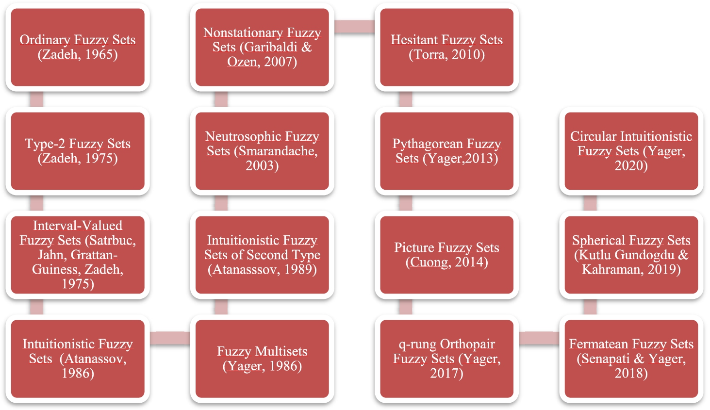
Fuzzy sets theory was developed by Zadeh (1965) in 1965 and the extensions of these ordinary fuzzy sets (OFSs) have been developed by numerous fuzzy set researchers. These fuzzy set extensions have been used in estimating, decision making, engineering economics, and controlling together with other intelligent systems. The extensions of ordinary fuzzy sets can be given as type-2 fuzzy sets in Zadeh (1975), intuitionistic fuzzy sets (IFSs) in Atanassov (1986), fuzzy multisets in Yager (1986), intuitionistic fuzzy sets of second type in Atanassov (1989), neutrosophic sets (NSs) in Smarandache (1999), nonstationary fuzzy sets in Garibaldi and Ozen (2007), hesitant fuzzy sets (HFSs) in Torra (2010), Pythagorean fuzzy sets (PFSs) in Yager (2013), picture fuzzy sets in Cuong (2014), q-rung orthopair fuzzy sets (q-ROFs) in Yager (2017), fermatean fuzzy sets (FFSs) in Senapati and Yager (2020), spherical fuzzy sets (SFSs) in Kutlu Gündoğdu and Kahraman (2019) and circular intuitionistic fuzzy sets (C-IFSs) in Atanassov (2020). In Fig. 1, the historical progress of the fuzzy set theory is given.
Fig. 1
Fuzzy set extensions.
Consideration of vagueness in the definition of membership functions is an old issue first time handled by Zadeh (1975). Type-2 fuzzy sets, interval-valued fuzzy sets and hesitant fuzzy sets try to incorporate this vagueness into their models. Similarly, Atanassov (2020) developed C-IFSs as an extension of IFSs in order to handle this issue. A circle around the single valued intuitionistic fuzzy number is defined by a radius r. In this study, the main aim and contribution is to introduce a new extension of PW analysis with interval-valued intuitionistic fuzzy sets (IVIF) and C-IFSs.
The estimation of investment parameters generally involves uncertainty and vagueness. This uncertainty is best handled by the fuzzy set theory in the literature. Most of the publications on fuzzy engineering economics employ ordinary fuzzy sets. However, there are some papers employing intuitionistic fuzzy sets, Pythagorean fuzzy sets, neutrosophic sets, hesitant fuzzy sets, type-2 fuzzy sets, and fermatean fuzzy sets in the investment analysis techniques. In the following, we present the review results on fuzzy PW analysis. Kahraman et al. (1995) presented financial models based on some discounting techniques such as fuzzy equivalent uniform annual worth and fuzzy PW analyses. Iliev and Fustik (2003) used fuzzy net present analysis in evaluating hydroelectric projects based on fuzzy profitability index. This model was created by using triangular fuzzy numbers. Omitaomu et al. (2004) used present value model with triangular fuzzy numbers in the evaluation of information system projects. Kahraman et al. (2004) proposed fuzzy present worth based fuzzy models for quantifying manufacturing flexibility. The fuzzy model included uncertain cash flows and discount rates that were handled as triangular fuzzy numbers. Kahraman and Kaya (2008) studied equivalent fuzzy annual worth analysis in investment assessment. Matos and Dimitrovski (2008) introduced studies using equivalent uniform annual worth analysis with trapezoidal fuzzy numbers. Kuchta (2008) presented fuzzy PW analysis applications in optimization. Dimitrovski and Matos (2008) introduced uncorrelated and correlated cash flows in fuzzy PW analysis with arithmetic operations. Shahriari (2011) proposed a fuzzy net present value methodology that uses triangular fuzzy numbers in investment analysis. Kahraman et al. (2015) presented hesitant and intuitionistic fuzzy present and annual worth analyses. These developed methods use triangular hesitant fuzzy data, triangular intuitionistic fuzzy data, interval-valued hesitant data, and interval-valued intuitionistic fuzzy data in engineering economic problems for better forecasting. Kahraman et al. (2018a) introduced Pythagorean PW analysis for investment decision problems. Sarı and Kahraman (2017) applied net PW analysis with type-2 fuzzy sets. One of the PW analysis papers which uses neutrosophic sets belongs to Aydin et al. (2018). They introduced simplified neutrosophic PW analysis. The investment parameters’ membership functions were defined by neutrosophic sets. The method was compared with classical and intuitionistic fuzzy PW analysis. Kahraman et al. (2018b) proposed ordinary fuzzy PW analysis, type-2 fuzzy PW analysis, intuitionistic fuzzy PW analysis, and hesitant fuzzy PW analysis in wind energy investment analysis. Aydin and Kabak (2020) developed future and present worth techniques in investment analysis with neutrosophic sets. Sergi and Sari (2021) extended PW analysis with fermatean fuzzy sets. The literature review is summarized in Table 1.
Table 1
Fuzzy PW analysis publications.
| Authors | Year | Type of fuzzy sets | Problem | Publication type |
| Kahraman et al. (1995) | 1995 | OFSs | Fuzzy flexibility evaluation | Conference paper |
| Iliev and Fustik (2003) | 2003 | OFSs | Hydroelectric project economical evaluation | Conference paper |
| Omitaomu et al. (2004) | 2004 | OFSs | Information system project for engineering economic analysis | Conference paper |
| Kahraman et al. (2004) | 2004 | OFSs | Fuzzy present worth models a for quantifying manufacturing flexibility | Article |
| Kahraman and Kaya (2008) | 2008 | OFSs | Fuzzy equivalent annual worth analysis in investment assessment | Book chapter |
| Matos and Dimitrovski (2008) | 2008 | OFSs | Fuzzy equivalent uniform annual worth analysis | Book chapter |
| Kuchta (2008) | 2008 | OFSs | Project selection optimization problem fuzzy net present value analysis | Book chapter |
| Dimitrovski and Matos (2008) | 2008 | OFSs | Uncorrelated and correlated cash flow in fuzzy PW analysis | Book chapter |
| Shahriari (2011) | 2011 | OFSs | Triangular fuzzy net present value for projects presentation | Book chapter |
| Kahraman et al. (2015) | 2015 | HFSs & Triangular hesitant data sets Interval-valued intuitionistic fuzzy sets & Triangular interval-valued intuitionistic fuzzy sets | Hesitant and intuitionistic fuzzy present worth and annual worth analyses | Article |
| Kahraman et al. (2018a) | 2018 | PFSs | Pythagorean fuzzy PW analysis in investments. | Conference paper |
| Sarı and Kahraman (2017) | 2017 | Type-2 fuzzy sets | Solid waste collection system for selection between roadside and underground waste bins. | Book chapter |
| Aydin et al. (2018) | 2018 | NSs | Investment evaluation problem with present value analysis. | Article |
| Kahraman et al. (2018b) | 2018 | OFSs Type-2 fuzzy sets HFSs | Ordinary fuzzy PW analysis, type-2 fuzzy PW analysis, intuitionistic fuzzy PW analysis, and hesitant fuzzy PW analysis | Book chapter |
| Aydin and Kabak (2020) | 2020 | NSs | Single valued neutrosophic present and future worth analysis | Article |
| Sergi and Sari (2021) | 2021 | FFSs | Fermatean fuzzy net PW analysis | Conference paper |
This paper is organized as follows: In Section 2, preliminaries of IVIF and C-IFSs are given. In Section 3, interval-valued intuitionistic fuzzy PW analysis extension is given. In Section 4, circular intuitionistic fuzzy PW analysis extension is given. In Section 5, a real life problem is solved with these proposed extensions in order to show the applicability of these proposed methods with a sensitivity analysis. Finally, conclusion is given in Section 6 with future suggestions.
2Preliminaries
In this section, the preliminaries of interval-valued intuitionistic fuzzy sets and C-IFSs are given with definitions.
2.1Interval-Valued Intuitionistic Fuzzy Sets
Intuitionistic fuzzy sets (IFSs) (Atanassov, 1986) were introduced by Atanassov in 1986. IVIFSs are an extension of IFSs that is developed by Atanassov and Gargov (1989) which have extensively been employed in the literature. IVIF numbers’ preliminaries are summarized in the following:
Definition 1.
Let X be a non-empty set. An IVIF set in X is an object
(1)
Definition 2.
Let
(2)
(3)
Definition 3.
Let
(4)
Definition 4.
Let
(5)
Definition 5.
Let
(6)
Definition 6.
Let
(7)
2.2Circular Intuitionistic Fuzzy Sets
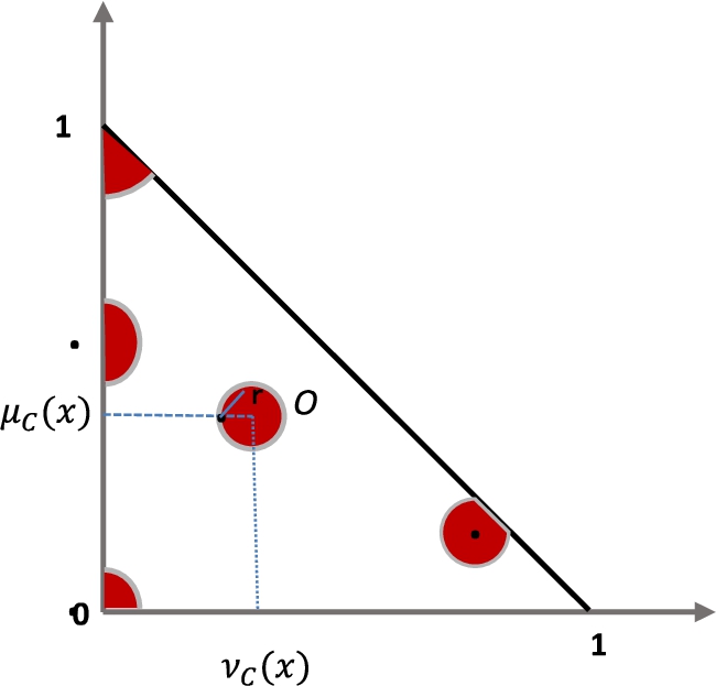
C-IFSs are introduced by Atanassov (2020) as an extension of the IFSs which each element is represented by a circle with radius r. C-IFSs is defined in Definition 8.
Definition 8.
Let E be a fixed universe. A C-IFS
(9)
(10)
The degree of indeterminacy is calculated as in Eq. (11):
(11)
In contrast with the standard IFSs, where each element is represented by a point in the intuitionistic fuzzy interpretation triplet, each element in C-IFSs is represented by a circle with centre
Definition 9.
In an IFS
(12)
Then, the radius of the
(13)
(14)
Definition 10.
Let’s have five circle forms as it is shown in Fig. 2, where the basic geometric interpretation of C-IFS is given.
(15)
(16)
C-IFSs is an extension of the standard IFSs and each standard IFS has the form
Fig. 2
C-IFS geometrical representation.
Definition 11.
Let
(17)
(18)
(19)
(20)
(21)
(22)
(23)
(24)
Aggregation of the intuitionistic fuzzy numbers is realized by using Definition 12.
3Interval-Valued Intuitionistic Fuzzy PW Analysis
The parameters of
(26)
(27)
(28)
(29)
(30)
(31)
Aggregation of IVIF numbers is performed by Eq. (25). Later, parameter values can be computed by multiplying the defuzzified values of membership functions with parameter values. The score function and defuzzification function of memberships are used for obtaining crisp values for each parameter. After defuzzification process the present worth is obtained by Eq. (32):
(32)
4Circular Intuitionistic Fuzzy PW Analysis
The parameters of FC, SV, AB, AC, i, and n are given by circular intuitionistic fuzzy numbers (CIFN) as in Eqs. (33)–(38):
(33)
(34)
(35)
(36)
(37)
(38)
In this method, aggregation of IFSs is performed by Eq. (25).
Later, parameter values can be computed by multiplying the defuzzified values of membership functions with parameter values. The score function and defuzzification function of memberships are used for obtaining crisp values for each parameter. After defuzzification process the present worth is obtained by Eq. (39):
(39)
5Application
A water treatment device will be purchased by a local municipality. The interval-valued intuitionistic fuzzy data of this device are given in Table 2. Three experts having different experiences assign three different intervals for each of investment parameters and determine their interval-valued intuitionistic fuzzy membership and non-membership degrees. w values in Table 2 represent the weights of experts based on their experience levels.
Table 2
Interval-valued intuitionistic fuzzy parameters.
| Parameter | Expert | w | Alternative | |
| First cost | E1 | 0.5 | ||
| 0.2 | ||||
| 0.3 | ||||
| E2 | 0.25 | |||
| 0.45 | ||||
| 0.3 | ||||
| E3 | 0.35 | |||
| 0.3 | ||||
| 0.35 | ||||
| Annual benefit | E1 | 0.5 | ||
| 0.2 | ||||
| 0.3 | ||||
| E2 | 0.25 | |||
| 0.45 | ||||
| 0.3 | ||||
| E3 | 0.35 | |||
| 0.3 | ||||
| 0.35 | ||||
| Annual cost | E1 | 0.5 | ||
| 0.2 | ||||
| 0.3 | ||||
| E2 | 0.25 | |||
| 0.45 | ||||
| 0.3 | ||||
| E3 | 0.35 | |||
| 0.3 | ||||
| 0.35 | ||||
| Salvage value | E1 | 0.5 | ||
| 0.2 | ||||
| 0.3 | ||||
| E2 | 0.25 | |||
| 0.45 | ||||
| 0.3 | ||||
| E3 | 0.35 | |||
| 0.3 | ||||
| 0.35 | ||||
| Interest rate | E1 | 0.5 | ||
| 0.2 | ||||
| 0.3 | ||||
| E2 | 0.25 | |||
| 0.45 | ||||
| 0.3 | ||||
| E3 | 0.35 | |||
| 0.3 | ||||
| 0.35 | ||||
| Life | E1 | 0.5 | ||
| 0.2 | ||||
| 0.3 | ||||
| E2 | 0.25 | |||
| 0.45 | ||||
| 0.3 | ||||
| E3 | 0.35 | |||
| 0.3 | ||||
| 0.35 |
We apply two levels of aggregation: Aggregation within each parameter and aggregation between parameters. In Table 3, the aggregated membership functions and expected weighted interval-values within each parameter are given. Then, aggregation between parameters is applied. For both of aggregation levels, Eq. (4) is used.
Table 3
Aggregation within each parameter.
| Parameter | Experts | Experts’ weights | Weighted interval-values | Aggregated membership functions | |
| FC | E1 | 0.4 | 216000 | 258000 | |
| E2 | 0.25 | 221000 | 260500 | ||
| E3 | 0.35 | 220000 | 260000 | ||
| AB | E1 | 0.4 | 44000 | 54000 | |
| E2 | 0.25 | 45250 | 55250 | ||
| E3 | 0.35 | 45000 | 55000 | ||
| AC | E1 | 0.4 | 14000 | 24000 | |
| E2 | 0.25 | 15250 | 25250 | ||
| E3 | 0.35 | 15000 | 25000 | ||
| SV | E1 | 0.4 | 88000 | 108000 | |
| E2 | 0.25 | 90500 | 110500 | ||
| E3 | 0.35 | 90000 | 78500 | ||
| IR | E1 | 0.4 | 0.088 | 0.108 | |
| E2 | 0.25 | 0.091 | 0.111 | ||
| E3 | 0.35 | 0.09 | 0.11 | ||
| n | E1 | 0.4 | 20.8 | 22.8 | |
| E2 | 0.25 | 22.1 | 25.05 | ||
| E3 | 0.35 | 21 | 25 | ||
Expected value calculations are given in Table 4. For instance, the value
Table 4
Values after aggregation within each parameter.
| Parameter | Expected interval-values | Aggregated membership functions |
| FC | ||
| AB | ||
| AC | ||
| SV | ||
| IR | ||
| Life |
The aggregation between parameters is the next step. Lower and upper
Now, circular intuitionistic fuzzy
Table 5
Circular intuitionistic fuzzy parameters.
| Parameters | Experts | W | Alternative | Membership function | Within aggregated membership functions ( | r | |
| First Cost | E1 | 0.5 | 0.486 | 0.627 | |||
| 0.2 | 0.592 | ||||||
| 0.3 | 0.627 | ||||||
| E2 | 0.25 | 0.020 | 0.153 | ||||
| 0.45 | 0.097 | ||||||
| 0.3 | 0.153 | ||||||
| E3 | 0.35 | 0.018 | 0.129 | ||||
| 0.3 | 0.122 | ||||||
| 0.35 | 0.129 | ||||||
| Annual Benefit | E1 | 0.5 | 0.048 | 0.093 | |||
| 0.2 | 0.093 | ||||||
| 0.3 | 0.022 | ||||||
| E2 | 0.25 | 0.062 | 0.080 | ||||
| 0.45 | 0.080 | ||||||
| 0.3 | 0.062 | ||||||
| E3 | 0.35 | 0.041 | 0.080 | ||||
| 0.3 | 0.101 | ||||||
| 0.35 | 0.041 | ||||||
| Annual Cost | E1 | 0.5 | 0.061 | 0.151 | |||
| 0.2 | 0.151 | ||||||
| 0.3 | 0.010 | ||||||
| E2 | 0.25 | 0.100 | 0.160 | ||||
| 0.45 | 0.066 | ||||||
| 0.3 | 0.160 | ||||||
| E3 | 0.35 | 0.315 | 0.315 | ||||
| 0.3 | 0.200 | ||||||
| 0.35 | 0.145 | ||||||
| Salvage Value | E1 | 0.5 | 0.048 | 0.093 | |||
| 0.2 | 0.093 | ||||||
| 0.3 | 0.023 | ||||||
| E2 | 0.25 | 0.133 | 0.133 | ||||
| 0.45 | 0.075 | ||||||
| 0.3 | 0.029 | ||||||
| E3 | 0.35 | 0.176 | 0.177 | ||||
| 0.3 | 0.036 | ||||||
| 0.35 | 0.177 | ||||||
| Interest Rate | E1 | 0.5 | 0.039 | 0.105 | |||
| 0.2 | 0.105 | ||||||
| 0.3 | 0.025 | ||||||
| E2 | 0.25 | 0.144 | 0.144 | ||||
| 0.45 | 0.002 | ||||||
| 0.3 | 0.139 | ||||||
| E3 | 0.35 | 0.090 | 0.090 | ||||
| 0.3 | 0.052 | ||||||
| 0.35 | 0.052 | ||||||
| Life | E1 | 0.5 | 0.032 | 0.085 | |||
| 0.2 | 0.085 | ||||||
| 0.3 | 0.031 | ||||||
| E2 | 0.25 | 0.046 | 0.059 | ||||
| 0.45 | 0.059 | ||||||
| 0.3 | 0.055 | ||||||
| E3 | 0.35 | 0.034 | 0.074 | ||||
| 0.3 | 0,074 | ||||||
| 0.35 | 0,043 |
A radius
Table 6
Expected parameters, aggregated membership functions and
| Parameters | Expected parameters | Within aggregated membership functions | |
| FC | 0.627 | ||
| AB | 0.101 | ||
| AC | 0.315 | ||
| SV | 0.177 | ||
| IR | 0.144 | ||
| Life | 0.085 |
For instance, the value of
Table 7 gives us the values of the investment parameters for both optimistic and pessimistic cases, separately.
Table 7
Optimistic and pessimistic membership functions.
| Parameters | Optimistic membership functions | Pessimistic membership functions |
| FC | ||
| AB | ||
| AC | ||
| SV | ||
| IR | ||
| Life | ||
| Membership functions (Max μ, Min ϑ for optimistic), (Max ϑ, Min μ for pessimistic) |
The score values for optimistic and pessimistic membership values are calculated as 1 and −0.741, respectively using Eq. (7).
Table 8 shows the average values of expected interval-values for the parameters.
Table 8
Expected interval-values and average values of parameters.
| Parameters | Expected interval-values | Midpoints |
| FC | 238,987.500 | |
| AB | 49,662.500 | |
| AC | 18,262.500 | |
| SV | 93,812.500 | |
| IR | 0.099 | |
| Life | 22.664 |
Based on the parameter values in Table 8,
(40)
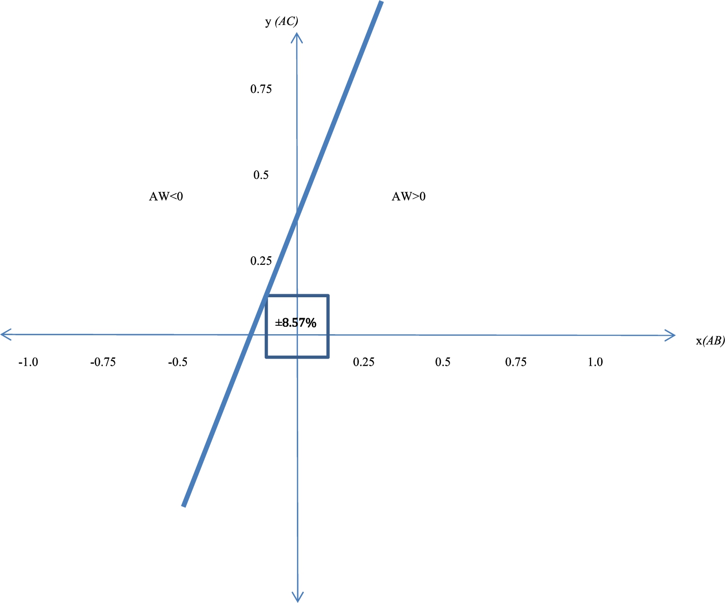
5.1Sensitivity Analysis
Sensitivity analysis is based on the midpoints of the parameters which are given in Table 8. The experts indicate that the most critical parameters are
(41)
(42)
Fig. 3 shows that possible
Fig. 3
Two parameters sensitivity analysis.
6Conclusion
C-IFSs (Atanassov, 2020) are the latest extension of IFSs based on the similar idea of type-2 fuzzy sets, which try to incorporate the vagueness and impreciseness of membership functions into the problem modelling. In this study, a comprehensive literature review has been presented and no investment analysis using circular intuitionistic fuzzy sets has been observed in this literature review. We have proposed new
References
1 | Atanassov, K., Gargov, G. ((1989) ). Interval-valued intuitionistic fuzzy sets. Fuzzy Sets and Systems, 31: , 343–349. |
2 | Atanassov, K.T. ((1986) ). Intuitionistic fuzzy sets. Fuzzy sets and Systems, 20: (1), 87–96. |
3 | Atanassov, K.T. ((1989) ). More on intuitionistic fuzzy sets. Fuzzy Sets and Systems, 33: (1), 37–45. |
4 | Atanassov, K.T. ((2020) ). Circular intuitionistic fuzzy sets. Journal of Ambient Intelligence and Smart Environments, 39: (5), 5981–5986. |
5 | Aydin, S., Kabak, M. ((2020) ). Investment analysis using neutrosophic present and future worth techniques. Journal of Intelligent and Fuzzy Systems, 38: (1), 627–637. |
6 | Aydin, S., Kahraman, C., Kabak, M. ((2018) ). Evaluation of investment alternatives using present value analysis with simplified neutrosophic sets. Engineering Economics, 29: (3), 254–263. |
7 | Cuong, B.C. ((2014) ). Picture fuzzy sets. Journal of Computer Science and Cybernetics, 30: (4), 409–420. |
8 | Dimitrovski, A., Matos, M. ((2008) ). Fuzzy present worth analysis with correlated and uncorrelated cash flows. In: Kahraman, C. (Ed.), Fuzzy Engineering Economics with Applications. Studies in Fuzziness and Soft Computing, Vol. 233: . Springer, Berlin, Heidelberg, pp. 11–41. |
9 | Garibaldi, J.M., Ozen, T. ((2007) ). Uncertain fuzzy reasoning: a case study in modelling expert decision making. IEEE Transactions on Fuzzy Systems, 15: (1), 16–30. |
10 | Iliev, A., Fustik, V. ((2003) ). Fuzzy logic approach for hydroelectric project evaluation. IFAC Proceedings Volumes 36: 7), 241–246. |
11 | Kahraman, C., Kaya, I. ((2008) ). Fuzzy equivalent annual-worth analysis and applications. In: Kahraman, C. (Ed.), Fuzzy Engineering Economics with Applications. Studies in Fuzziness and Soft Computing, Vol. 233: . Springer, Berlin, Heidelberg, pp. 71–81. |
12 | Kahraman, C., Tolga, E., Ulukan, Z. ((1995) ). Fuzzy flexibility analysis in automated manufacturing systems. In: IEEE Symposium on Emerging Technologies & Factory Automation, Vol. 3: , pp. 299–307. |
13 | Kahraman, C., Beskese, A., Ruan, D. ((2004) ). Measuring flexibility of computer integrated manufacturing systems using fuzzy cash flow analysis. Information Sciences, 168: (1–4), 77–94. |
14 | Kahraman, C., Çevik Onar, S., Öztayşi, B. ((2015) ). Engineering economic analyses using intuitionistic and hesitant fuzzy sets. Journal of Intelligent and Fuzzy Systems, 29: (3), 1151–1168. |
15 | Kahraman, C., Onar, S.C., Oztaysi, B. ((2018) a). Present worth analysis using Pythagorean fuzzy sets. In: Kacprzyk, J., Szmidt, E., Zadrożny, S., Atanassov, K., Krawczak, M. (Eds.), Advances in Fuzzy Logic and Technology 2017. EUSFLAT2017, IWIFSGN 2017. Advances in Intelligent Systems and Computing, Vol. 642: . Springer, Cham, pp. 336–342. https://doi.org/10.1007/978-3-319-66824-6_30. |
16 | Kahraman, C., Çevik Onar, S., Öztayşi, B., Sarıİ, U., İlbahar, E. ((2018) b). Wind energy investment analyses based on fuzzy sets. In: Kahraman, C., Kayakutlu, G. (Eds.), Energy Management—Collective and Computational Intelligence with Theory and Applications. Studies in Systems, Decision and Control, Vol. 149: . Springer, Cham. |
17 | Kuchta, D. ((2008) ). Optimization with fuzzy present worth analysis and applications. In: Kahraman, C. (Ed.), Fuzzy Engineering Economics with Applications. Studies in Fuzziness and Soft Computing, Vol. 233: . Springer, Berlin, Heidelberg, pp. 43–69. |
18 | Kutlu Gündoğdu, F., Kahraman, C. ((2019) ). Spherical fuzzy sets and spherical fuzzy TOPSIS method. Journal of Intelligent and Fuzzy Systems, 36: (1), 337–352. |
19 | Matos, M., Dimitrovski, A. ((2008) ). Case studies using fuzzy equivalent annual worth analysis. In: Kahraman, C. (Ed.), Fuzzy Engineering Economics with Applications. Studies in Fuzziness and Soft Computing, Vol. 233: . Springer, Berlin, Heidelberg, pp. 83–95. |
20 | Omitaomu, H.O., Nsofor, C.G., Badiru, A.B. ((2004) ). Integrative present value analysis model for evaluating information system projects. In: IIE Annual Conference and Exhibition, pp. 2065–2070. |
21 | Sarı, İ.U., Kahraman, C. ((2017) ). Economic analysis of municipal solid waste collection systems using type-2 fuzzy net present worth analysis. In: Intelligence Systems in Environmental Management: Theory and Applications. Springer, Cham, pp. 347–364. |
22 | Senapati, T., Yager, R.R. ((2020) ). Fermatean fuzzy sets. Journal of Ambient Intelligence and Humanized Computing, 11: , 663–674. |
23 | Sergi, D., Sari, I.U. ((2021) ). Fuzzy capital budgeting using fermatean fuzzy sets. In: Kahraman, C., Cevik Onar, S., Oztaysi, B., Sari, I., Cebi, S., Tolga, A. (Eds.), Intelligent and Fuzzy Techniques: Smart and Innovative Solutions. INFUS 2020. Advances in Intelligent Systems and Computing, Vol. 1197: . Springer, Cham. |
24 | Shahriari, M. ((2011) ). Mapping fuzzy approach in engineering economics. International Research Journal of Finance and Economics, 81: , 6–12. |
25 | Smarandache, F. ((1999) ). A Unifying Field in Logics. Neutrosophy: Neutrosophic Probability, Set and Logic. American Research Press, Rehoboth. |
26 | Torra, V. ((2010) ). Hesitant fuzzy sets. International Journal of Intelligent Systems, 25: (6), 529–539. |
27 | Wei, G., Wang, X. ((2007) ). Some geometric aggregation operators based on interval-valued intuitionistic fuzzy sets and their application to group decision making. In: 2007 International Conference on Computational Intelligence and Security. IEEE, Harbin, pp. 495–499. |
28 | Xu, Z. ((2007) ). Methods for aggregating interval-valued intuitionistic fuzzy information and their application to decision making. Kongzhi Yu Juece/Control and Decision, 22: (2), 215–219. |
29 | Xu, Z.S. ((2010) ). A distance measure based method for interval-valued intuitionistic fuzzy multi-attribute group decision making. Information Sciences, 180: , 181–190. |
30 | Xu, Z.S., Yager, R.R. ((2006) ). Some geometric aggregation operators based on intuitionistic fuzzy sets. International Journal of General Systems, 35: , 417–433. |
31 | Yager, R.R. ((1986) ). On the theory of bags. International Journal of General System, 13: (1), 23–37. |
32 | Yager, R.R. ((2013) ). Pythagorean fuzzy subsets. In: Joint IFSA World Congress and NAFIPS Annual Meeting (IFSA/NAFIPS), 24–28 June, Edmonton, Canada, pp. 57–61. |
33 | Yager, R.R. ((2017) ). Generalized orthopair fuzzy sets. IEEE Transactions on Fuzzy Systems, 25: (5), 1222–1230. |
34 | Zadeh, L.A. ((1965) ). Fuzzy sets. Information Control, 8: (3), 338–353. |
35 | Zadeh, L.A. ((1975) ). The concept of a linguistic variable and its application to approximate reasoning. Information Sciences, 8: (3), 199–249. |


