
A New Similarity Measure for Picture Fuzzy Sets and Its Application to Multi-Attribute Decision Making
Abstract
As an extension of intuitionistic fuzzy sets, picture fuzzy sets can deal with vague, uncertain, incomplete and inconsistent information. The similarity measure is an important technique to distinguish two objects. In this study, a similarity measure between picture fuzzy sets based on relationship matrix is proposed. The new similarity measure satisfies the axiomatic definition of similarity measure. It can be testified from a numerical experiment that the new similarity measure is more effective. Finally, we apply the proposed similarity measure to multiple-attribute decision making.
1Introduction
There is a lot of vague and uncertain information in the real world; Zadeh (1965) established the fuzzy set to handle this information. The fuzziness and uncertainty are characterized by assigning a membership degree to each element. But in reality, the single membership degree cannot adequately express the hesitancy of multiple information. Atanassov Atanassov (1986) developed the intuitionistic fuzzy set to eliminate such situations. Intuitionistic fuzzy set consists of the membership degree and the non-membership degree, the sum of which is not more than one. Intuitionistic fuzzy set has been widely used in pattern recognition (Chu et al., 2014; Chen and Chang, 2015; Dhivya and Sridevi, 2019; Luo et al., 2018), decision making (Chen et al., 2016; Li and Zeng, 2015; Ngan et al., 2018), clustering analysis (Khan and Lohani, 2016; Hwang et al., 2018; Jiang and Jin, 2019; Wang and Mao, 2018), image processing (Bustince et al., 2007; Xu et al., 2009) and so on. Intuitionistic fuzzy set has received extensive attention from the research community, but it is limited when dealing with ambiguous, uncertain, incomplete, and inconsistent information. For example, voting questions: all voting results can be grouped into four groups that are “vote for”, “abstain”, “vote against” and “refuse to vote”. Cuong (2013) presents the picture fuzzy set, which is composed of the positive, the negative, the neutral and the refusal membership degrees. It is more flexible than intuitionistic fuzzy set in dealing with such problems. Therefore, numerous studies related to picture fuzzy sets have become popular among various WEI domains. Wei et al. (2019) studied two aggregation operators of a picture fuzzy set, and applied it to the safety assessment of a construction project. Wei et al. (2021) developed some picture 2-tuple linguistic power Hamy mean aggregation operators based on the power average and power geometric operations, and used it for enterprise resource planning system selection. Zhang et al. (2020) extended multi-attributive border approximation area comparison method to the multiple attribute group decision making with picture 2-tuple linguistic numbers. Luo and Long (2021) propose some picture fuzzy geometric aggregation operators, and apply it to multi-attribute decision making questions.
As one of the research hotspots of picture fuzzy sets, similarity measure is used to assess the similarity between two objects. Distance measures and similarity measures are complementary and are used to illustrate differences between two matters. Recently, the exploration of distance measures and similarity measures between picture fuzzy sets have presented a lot of achievements. Cuong (2013) gave the Hamming distance and Euclidean distance. Singh et al. (2018) developed two distance measures with parameters, which contain normalized Hamming distance, normalized Euclidean distance and normalized Hausdorff distance as special situations. Based on these distances, Singh et al. studied a new similarity measure and applied it to assess flood disaster risk. Son (2016) introduced a generalized distance measure, and applied it to clustering issues. Dutta (2017) pointed out that Son’s distance measure has limitations, presented a new distance measure and used it for medical diagnostic problems. Liu and Zeng (2019) explored some picture fuzzy weighted, ordered weighted and hybrid weighted distance measures, and used them for multi-attribute group decision making. Dinh and Thao (2018) presented several distance and dissimilarity measures and applied them to pattern recognition and decision making problems. Wei (2016) presented picture fuzzy cross-entropy, and used it for multi-attribute decision making questions. Wei et al. (2018) introduced cosine projection model, and employed it to decision making problems. Wei and Gao (2018) proposed a normalized Dice similarity measure with parameter, and applied it to building material recognition. Wei (2017b) proposed a similarity measure based on cosine function, and used it for strategic decision making issues. Luo and Zhang (2020) proposed a similarity measure based on the constituent functions of a picture fuzzy set, and applied it to pattern recognition.
However, existing similarity measures do not take into account the relationship between four functions of the picture fuzzy set, which will lead to unreasonable results in some cases (see Example 4.1). This study introduces a new similarity measure between picture fuzzy sets, which not only considers the four functions of picture fuzzy sets but also considers the relationship between them. In particular, the relationship between the refusal membership function and positive membership function, neutral membership function, negative membership function are considered separately. A numerical example shows that the proposed similarity measure can conquer the defect of some existing ones. When applied to multi-attribute decision making, reasonable and effective results can be obtained. The rest of this paper consists of the following. In Section 2, we review primary concepts and properties about picture fuzzy sets. In Section 3, a novel similarity measure based on relationship matrix is proposed. In Section 4, the proposed similarity measure is used for multi-attribute decision making. Section 5 is the conclusion.
2Preliminaries
In this part, some basic concepts of picture fuzzy sets are reviewed. We list some existing similarity measures that will be used later.
Definition 2.1
Definition 2.1(See Atanassov, 1986).
A intuitionistic fuzzy set A on universe X is an object of the form:
Definition 2.2
Definition 2.2(See Cuong, 2013).
A picture fuzzy set A on universe X is an object of the form:
Let
Definition 2.3
Definition 2.3(See Cuong et al., 2016).
Let
(1)
(2)
(3)
Definition 2.4
Definition 2.4(See Singh et al., 2018).
Let
Let
Dinh and Thao’s similarity measures (Dinh and Thao (2018)):
(1)
(2)
(3)
(4)
(5)
(6)
(7)
(8)
(9)
(10)
(11)
Palash’s similarity measures (Dutta, 2017):
(12)
3A New Similarity Measure for Picture Fuzzy Sets
In this section, we will give a new similarity measure between picture fuzzy sets based on a relationship matrix, which is composed of the values of the relationship between positive membership, neutral membership, negative membership and refusal membership, respectively.
Theorem 3.1.
Let
(13)
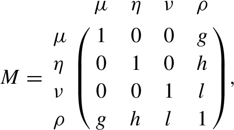
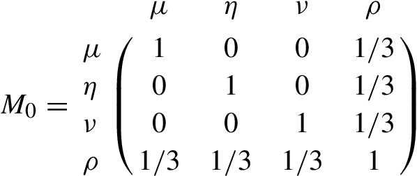
In this relationship matrix, we know that the relation value between positive membership and positive membership is 1. Similarly, the relation value between neutral memberships, negative memberships, refusal memberships are 1. Since the three component functions of picture fuzzy set are independent of each other, the relation value among positive membership, neutral membership and negative membership are 0. We assume that the values of the relationship between the refusal membership and positive membership, neutral membership, negative membership are g, h, l, respectively. It’s clear that g, h, l are not greater than one, and they add up to one.
Proof.
Let
Taking a close explanation of the similarity measure
(S1) For
(S2) Obviously,
(S3)
(S4) Let
In the same way, we can get
(1) Suppose that
(2) Suppose that
(3) Suppose that
Furthermore, picture fuzzy sets
(4)
(5)
(6)
(7)
(8)
(9)
Similarly, these cases can be proved.
Remark 3.1.
Let
(14)
 .
.Remark 3.2.
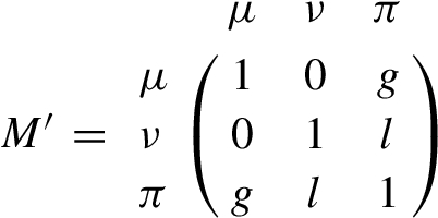
If picture fuzzy sets A and B degenerate into intuitionistic fuzzy sets, the similarity measure
(15)
 , and
, and Remark 3.3.
For
Theorem 3.2.
Let
(16)
4Applications
In this section, a numerical example is constructed. Some of the existing similarity measures cannot produce rational results, while the proposed similarity measure can get a logical result. Then we apply the proposed similarity measure to multi-attribute decision making.
4.1Numerical Comparisons
Example 4.1.
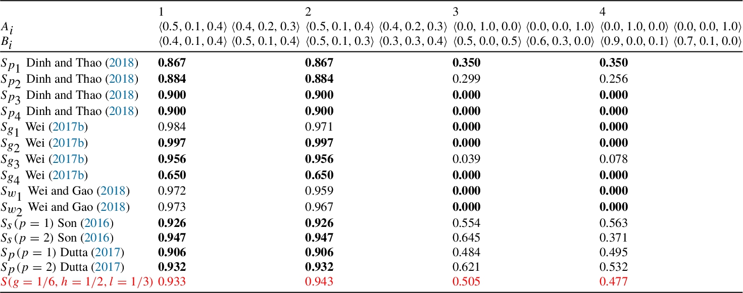
By comparing the first pairs of picture fuzzy sets
Table 1
Comparisons of different similarity measures (counter-intuitive cases are in bold type).
4.2Algorithm and Applications
4.2.1Algorithm for Multi-Attribute Decision Making
Let
Step 1. Attributes may be divided into two types: cost attribute
Step 2. Let
Step 3. Calculate the similarity measure
Step 4. Rank all alternatives
4.2.2Applications for Multi-Attribute Decision Making
Example 4.2.
Joshi and Kumar (2018) consider an Indian multinational is planning its financial strategy in line with the group’s strategic objectives. After preliminary screening, four alternatives were obtained and determined as:
Step 1.
Table 2
Picture fuzzy decision matrix.
Step 2. The ideal alternative is
Table 3
Normalized picture fuzzy decision matrix.
Step 3. We calculate the similarity measure
Table 4
The results of similarity measure
| 0.711 | 0.703 | |
| 0.773 | 0.771 | |
| 0.715 | 0.708 | |
| 0.641 | 0.627 |
Table 5
Ranking results.
| Methods | Ranking order |
Step 4. The maximal similarity is the best one, the ranking results are shown in Table 5.
Table 6
Comparisons with other methods.
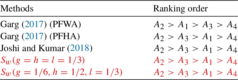
From the above results, it is clear that the best financial strategy is
Example 4.3.
Wei et al. (2018) consider an organization intends to select a promising emerging technology commercial enterprise. After their preliminary screening five enterprises are expressed as
Table 7
Normalized picture fuzzy decision matrix.
Step 1.
Table 8
The results of similarity measure
| 0.649 | 0.652 | |
| 0.717 | 0.721 | |
| 0.718 | 0.724 | |
| 0.604 | 0.606 | |
| 0.626 | 0.629 |
Step 2. The ideal alternative is
Step 3. We calculate the similarity measure
Step 4. The maximal similarity is the best one, we get ranking results in Table 9.
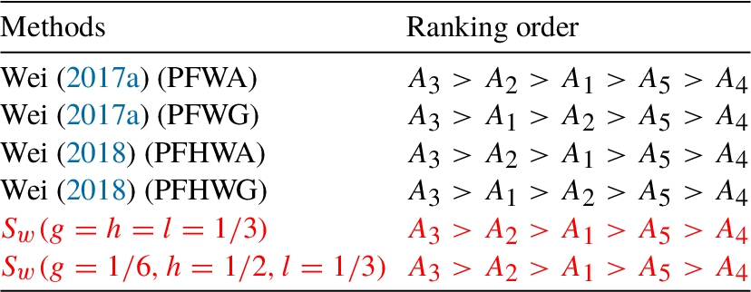
From the above discussion, it is clear that the most promising enterprise is
Table 9
Ranking results.
| Methods | Ranking order |
Table 10
Comparisons with other methods.
Example 4.4.
Table 11
Normalized picture fuzzy decision matrix.
Consider a supplier who wants to choose a construction company to work with. After their preliminary screening three companies are expressed as
Step 1.
Step 2. The ideal alternative is
Step 3. We calculate similarity measure
Table 12
The results of similarity measure
| 0.757 | 0.739 | |
| 0.749 | 0.734 | |
| 0.657 | 0.645 |
Table 13
Ranking results.
| Methods | Ranking order |
Step 4. The maximal similarity is the best alternative, we get the ranking results in Table 13.
Table 14
Comparisons with other methods.
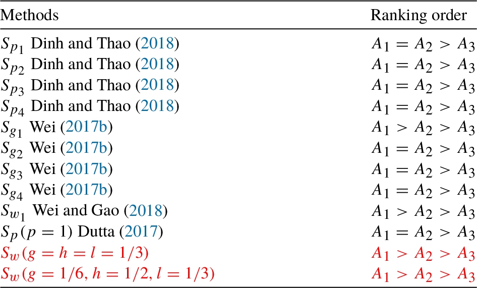
From the above discussion, it is clear that the best company is
4.3Analysis and Discussion
In practical problems, we find that the proposed method can also solve some multi-attribute decision making problems which can be solved by existing methods. The proposed method can solve some multi-attribute decision making problems which cannot be solved by existing methods. It shows that the method we proposed is reasonable and superior. Furthermore, we find some existing methods can’t make decisions, because the similarity measure formulas only carry out simple operations on positive membership, neutral membership and negative membership, and it may result in the calculation result of similarity between picture fuzzy sets and other different picture fuzzy sets being the same. The new method based on relational matrix is proposed, which overcomes the defects mentioned above and achieves good results in multi-attribute decision making.
5Conclusions
In this study, we develop a novel similarity measure between picture fuzzy sets based on the relationship matrix, which not only considers the four membership functions of picture fuzzy sets but also the relations between them. Particularly, the relationship between the refusal membership and positive membership, neutral membership, negative membership are explored. The proposed similarity measure satisfies the axiom definition of similarity measure. A numerical comparison shows that the proposed similarity measure is more effective than other methods in distinguishing picture fuzzy sets. It can conquer defects of some existing similarity measures. Moreover, in multi-attribute decision experiments, the decision results show that the proposed similarity measure is valid and superior.
Acknowledgement
The authors would like to thank the Editor and anonymous reviewers for their valuable comments and suggestions.
References
1 | Atanassov, K. ((1986) ). Intuitionistic fuzzy sets. Fuzzy Sets and Systems, 20: , 87–96. |
2 | Bustince, H., Barrenechea, E., Pagola, M. ((2007) ). Image thresholding using restricted equivalence functions and maximizing the measures of similarity. Fuzzy Sets and Systems, 158: , 496–516. |
3 | Chen, S.M., Chang, C.H. ((2015) ). A novel similarity measure between Atanassov’s intuitionistic fuzzy sets based on transformation techniques with applications to pattern recognition. Information Sciences, 291: , 96–114. |
4 | Chen, S.M., Cheng, S.H., Chiou, C.H. ((2016) ). Fuzzy multiattribute group decision making based on intuitionistic fuzzy sets and evidential reasoning methodology. Information Fusion, 27: , 215–227. |
5 | Chu, C.H., Hung, K.C., Julian, P.A. ((2014) ). Complete pattern recognition approach under Atanassov’s intuitionistic fuzzy sets. Knowledge-Based Systems, 66: , 36–45. |
6 | Cuong, B. (2013). Picture fuzzy sets-sets – a new concept for computational intelligence problems. In: Proceedings of the Third World Congress on Information and Communication Technologies (WICT 2013), Hanoi. IEEE, pp. 1–6. |
7 | Cuong, B., Kreinovitch, V., Ngan, R.T. (2016). A classification of representable t-norm operators for picture fuzzy sets. In: Eighth International Conference on Knowledge and Systems Engineering (KSE 2016), Hanoi. IEEE, pp. 19–24. |
8 | Dhivya, J., Sridevi, B. ((2019) ). A novel similarity measure between intuitionistic fuzzy sets based on the mid points of transformed triangular fuzzy numbers with applications to pattern recognition and medical diagnosis. A Journal of Chinese Universities, 34: , 229–252. |
9 | Dinh, N.V., Thao, N.X. ((2018) ). Some measures of picture fuzzy sets and their application in multi-attribute decision making. Mathematical Sciences and Computing, 3: , 23–41. |
10 | Dutta, P. ((2017) ). Medical diagnosis via distance measures on picture fuzzy sets. Advances in Modelling and Analysis A, 54: , 137–152. |
11 | Garg, H. ((2017) ). Some picture fuzzy aggregation operators and their applications to multicriteria decision making. Research Article – Systems Engineering, 42: , 5275–5290. |
12 | Hwang, C.M., Yang, M.S., Hung, W.L. ((2018) ). New similarity measure of intuitionistic fuzzy sets based on the jaccard index with its application to clustering. International Journal of Intelligent Systems, 38: (8), 1672–1688. |
13 | Jiang, Q., Jin, X. ((2019) ). A new similarity/distance measure between intuitionistic fuzzy sets based on the transformed isosceles triangles and its applications to pattern recognition. Expert Systems with Applications, 116: , 439–453. |
14 | Joshi, D., Kumar, S. (2018). An approach to multi-criteria decision making problems using dice similarity measure for picture fuzzy sets. In: Communications in Computer and Information Science, 1–6. |
15 | Khan, M.S., Lohani, Q.M.D. ((2016) ). A similarity measure for atanassov intuitionistic fuzzy sets and its application to clustering. In: 2016 International Workshop on Computational Intelligence (IWCI), pp. 232–239. https://doi.org/10.1109/IWCI.2016.7860372. |
16 | Li, J.H., Zeng, W.Y. ((2015) ). A new dissimilarity measure between intuitionistic fuzzy sets and its application in multipile attribute decision making. International Journal of Fuzzy Systems, 29: , 1311–1320. |
17 | Liu, M., Zeng, S.Z. ((2019) ). Picture fuzzy weighted distance measures and their applications to investment selection. Amfiteatru Economic, 21: , 682–695. |
18 | Luo, M.X., Zhang, Y. ((2020) ). A new similarity measure between picture fuzzy sets and its application. Engineering Applications of Artificial Intelligence, 96: , 103956. |
19 | Luo, M.X., Long, H.F. ((2021) ). Picture fuzzy geometric aggregation operators based on a trapezoidal fuzzy number and its application. Symmetry, 13(1): , 119. |
20 | Luo, X., Li, W., Zhao, W. ((2018) ). Picture fuzzy weighted distance measures and their applications to investment selection. Applied Intelligence, 48: , 2792–2808. |
21 | Ngan, R.T., Song, L.H., Cuong, B.C. ((2018) ). H-max distance measure of intuitionistic fuzzy sets in decision making. Applied Soft Computing, 69: , 393–425. |
22 | Singh, P., Mishra, N.K., Kumar, M., Saxena, S., Singh, V. ((2018) ). Risk analysis of flood disaster based on similarity measures in picture fuzzy environment. Afrika Matematika, 29: , 1019–1038. |
23 | Son, L.H. ((2016) ). Generalized picture distance measure and applications to picture fuzzy clustering. Applied Soft Computing, 46: , 284–295. |
24 | Song, Y.F., Wang, X.D., Lei, L., Quan, W., Huang, W.L. ((2016) ). An evidential view of similarity measure for Atanassov’s intuitionistic fuzzy sets. Journal of Intelligent and Fuzzy Systems, 31: , 1653–1668. |
25 | Wang, F., Mao, J. ((2018) ). Aggregation similarity measure based on intuitionistic fuzzy closeness degree and its application to clustering analysis. Journal of Intelligent and Fuzzy Systems, 35: , 609–625. |
26 | Wei, G.W. ((2016) ). Picture fuzzy cross-entropy for multiple attribute decision making problems. Journal of Business Economics and Management, 17: , 491–502. |
27 | Wei, G.W. ((2017) a). Picture fuzzy aggregation operators and their application to multiple attribute decision making. Journal of Intelligent and Fuzzy Systems, 33: , 713–724. |
28 | Wei, G.W. ((2017) b). Some cosine similarity measures for picture fuzzy sets and their applications to strategic decision making. Informatica, 144: , 547–564. |
29 | Wei, G.W. ((2018) ). Picture fuzzy hamacher aggregation operators and their application to multiple attribute decision making. Fundamenta Informaticae, 157: , 271–320. |
30 | Wei, G.W., Gao, H. ((2018) ). The generalized dice similarity measures for picture fuzzy sets and their applications. Informatica, 160: , 107–124. |
31 | Wei, G.W., Alsaadi, F.T., Hayat, T., Alsaedi, A. ((2018) ). Projection models for multiple attribute decision making with picture fuzzy information. International Journal of Machine Learning and Cybernetics, 9: , 491–502. |
32 | Wei, G.W., Zhang, S.Q., Lu, J.P., Wu, J., Wei, C. ((2019) ). An extended bidirectional projection method for picture fuzzy MAGDM and its application to safety assessment of construction project. IEEE Access, 7: , 166138–166147. |
33 | Wei, G.W., Wang, J., Gao, H., Wei, C. ((2021) ). Approaches to multiple attribute decision making based on picture 2-tuple linguistic power Hamy mean aggregation operators. RAIRO-Operations Research, 55: , 435–460. |
34 | Xu, S.P., Zhang, H., Jiang, S.L. ((2009) ). Image similarity measure based on intuitionistic fuzzy set. Pattern Recognition and Artificial Intelligence, 22: , 157–161. |
35 | Zadeh, L.A. ((1965) ). Fuzzy sets. Information Control, 8: , 338–353. |
36 | Zhang, S.Q., Wei, G.W., Alsaadi, F.E., Hayat, T., Wei, C., Zhang, Z.Z.P. ((2020) ). MABAC method for multiple attribute group decision making under picture 2-tuple linguistic environment. Soft Computing, 24: , 5819–5829. |


