Los Alamos chess game 2 (after P-K3) is solved; black wins in 21 moves

1.Problem

Los Alamos chess is a chess variant played on a 6×6 board without bishops, and with only six pawns on each side. It follows the standard rules of chess with three differences designed to further simplify the game: no pawn double-step moves (and therefore no en passant captures), no castling, and pawns may not be promoted to bishops. The initial board position is shown in Fig. 1. Both the reduction in book-keeping and the elimination of the bishops (clergy) lead to game also being known as “anti-clerical chess”.

The origin of Los Alamos chess dates back to the early 1950s, and the severe technical limitations of the MANIAC 1 computer. Following the success of the Manhattan Project in developing the atomic bomb, Robert Oppenheimer directed John von Neumann and Nick Metropolis to construct the first fully electronic computer to be installed at (what today is known as) Los Alamos National Laboratories in New Mexico, USA. Based on von Neumann’s earlier IAS machine running at the Institute for Advanced Studies in Princeton, MANIAC 1 could execute 10 thousand instructions per second, used 2,400 vacuum tubes, and had 1024 40-bit words (5000 bytes) of electrostatic Cathode Ray Tube (CRT) memory and 10K words of magnetic drum storage.

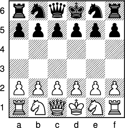
Fig. 1.

Opening position for (full) Los Alamos chess.

Although primitive in comparison to today’s hardware, this system allowed for the earliest experiments in computer chess and artificial intelligence. The simplifications of Los Alamos Chess enabled Mark Wells, Paul Stein and Stanisław Ulam to write the world’s first computer program for a chess-like game, Los Alamos chess (Fig. 2). This program could search 2 moves (4 ply) ahead, and took on average 12 minutes to ponder each move. Los Alamos chess’ use of a 6×6 board may have been driven as much by reliability as by capacity, as regular chess was estimated to require about 2 hours per move on MANIAC I (Kister et al., 1957), which operationally had a mean time between failures of about 5 hours.

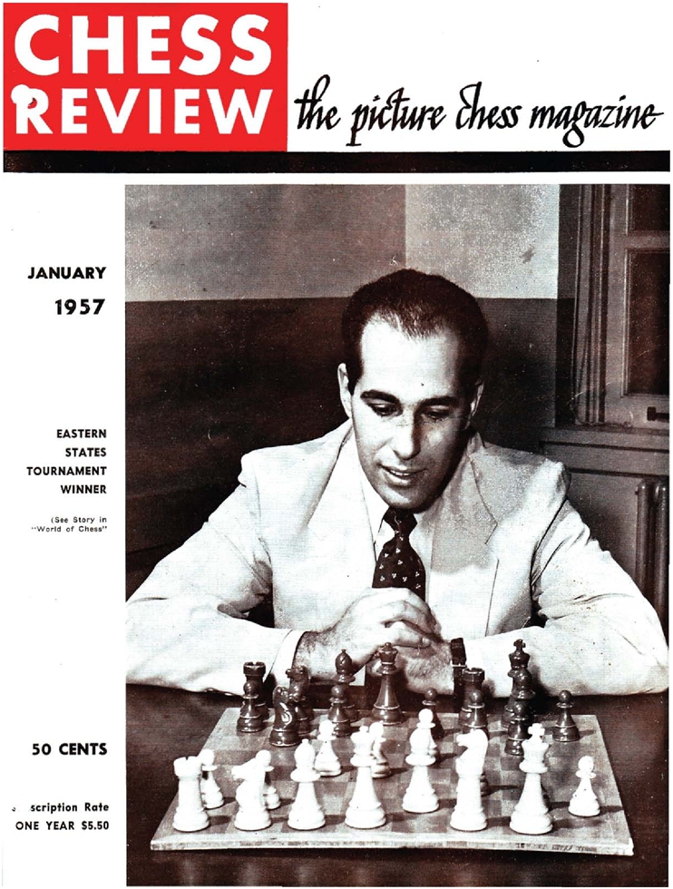
The first experiments in computer chess where published by Paul Stein and Stanisław Ulam in the January 1957 issue of Chess Review in an article entitled “Experiments in Chess on Electronic Computing Machines”. Stanisław Ulam is perhaps best known as one of the two co-inventors of the hydrogen bomb, and directed software development on the MANIAC 1. By an interesting co-incidence, the cover of this issue of Chess Review (Fig. 3) depicts the Eastern States Tournament Winner: Hans Berliner. Hans Berliner is famous in the world of computer chess, as the developer of the HiTech chess engine, inventor of the B∗ search algorithm, a chess master, and both a grand master and world champion in correspondence chess (Berliner, 1979-1985). It is tempting to speculate that the Stein and Ulam article first describing computer chess to the general public appearing in “his” issue may have been instrumental in Hans’ life long interest in computer chess.

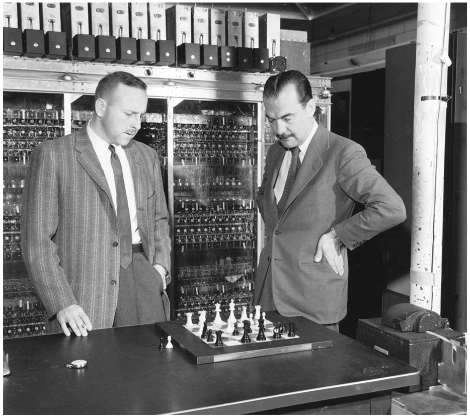
Fig. 2.

Paul Stein and Nick Metropolis play Los Alamos chess in front of MANIAC 1.

The article details the first three games played by MANIAC 1. Game 1 was MANIAC 1 playing against itself. Because the brute-force algorithms used by MANIAC 1 were completely deterministic, all machine-vs-machine games would produce this same sequence of moves. Game 2, the first game against a human opponent, was played against a strong chess player, Martin Kruskal of Princeton University, who played White, but to even the odds White played without a queen. In this game, Kruskal opened with P-K3 (also written as d2d3), and eventually won the game after 38 moves (75 ply). The third game was played against a beginner, a laboratory assistant who had been taught the rules of chess in the previous week. In this third game, MANIAC I playing White won in 23 moves (45 ply), marking the first time a computer had beaten a human opponent in a game of skill.

Fig. 3.

Hans Berliner on the front cover of the January 1957 issue of chess review, that contained Stein and Ulam’s first description of Los Alamos chess.

In this article, we use the term ‘Los Alamos Chess Game 2’ to denote not only the above landmark match, but also the minichess variant of Los Alamos chess where White plays without a queen. It was not previously known whether the material disadvantage for White, but with the first move advantage and slightly better initial mobility, is decisive under perfect play by both opponents.

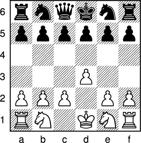
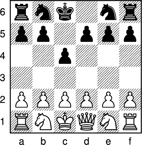
The board for Los Alamos chess game 2, after White’s opening move P-K3, with Black to move, as faced by MANIAC 1 is shown in Fig. 4. In Forsyth–Edwards notation (FEN) notation, this position is written as rnqknr/pppppp/6/3P2/PPP1PP/RN1KNR w - - 0 1 (Edwards, 1994). The main result of this paper is a game theoretic analysis of this position.

2.Methods

A two player game is weakly solved if there exists an algorithm that secures a win for either player, against any possible move by the opponent, from the beginning of the game. For this work, a weak solution or proof consists of a table of positions and their corresponding moves for one side, that covers all positions reachable from the starting “root” position under all possible counter-moves by the opponent, and each position eventually leads (without cycles) to a terminal checkmate. In computer science terminology, such a proof tree is actually a directed acyclic graph (DAG).

The effort involved in (weakly) solving a game depends upon a number of factors, including the size of the search space, the branching factor, the depth of the solution and the decision complexity (Allis, 1994). The number of unique chess games, the Shannon number, was first estimated by Claude Shannon to be about 10120 to demonstrate that solving chess by brute force is impractical (Shannon, 1950). The most recent upper bound on the number of possible regular 8×8 chess positions, as calculated by John Tromp, is about 8.7×1045 (Tromp, 2021). Modifying Tromp’s Haskell program to provide an estimate for Los Alamos chess yields an estimate of about 4×1029 possible positions, significantly simpler than regular chess, but higher than the about 5×1020 positions in checkers, which was weakly solved by Jonathan Schaeffer in 2007 (Schaeffer, 2008), and the about 1028 positions in Othello/Reversi, which was weakly solved by Hiroki Takizawa in 2023 (Takizawa, 2023). Likewise, the branching factor of Los Alamos chess, which is around 22, is roughly two thirds of the branching factor of regular chess, which is around 35. Go has a branching factor of 300, and Connect Four has a branching factor of 7. The largest chess variant solved prior to this work is Gardener’s minichess, which is played on a 5×5 board (Mhalla and Prost, 2013).

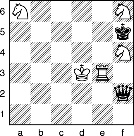
By convention many chess problems are posed as “White to move and win” and indeed many of the custom tools used/developed by the author made this assumption. Without loss of generality, the problem may be rephrased as a White to move (and win) problem, by reversing the board, as shown in Fig. 5 below. In Forsyth–Edwards notation this starting position is described as rnk1nr/pp1ppp/2p3/6/PPPPPP/RNKQNR w - - 0 1.

Fig. 4.

Los Alamos chess game 2 after P-K3, with black to move and win in 21 moves.

Solving this chess position involved several pieces of custom software, including traditional alpha-beta tree search (Campbell and Marsland, 1983), proof-number search (Breuker et al., 1994; Winands et al., 2003), Monte Carlo tree search (Coulom, 2007) and end-game tablebase generators, but the main recent workhorse was a slightly modified version of Fairy-Stockfish, developed by Fabian Fichter (Fichter, 2021). Fairy-Stockfish is chess variant engine derived from the computer chess champion chess engine Stockfish (originally written by Tord Romstad, Marco Costalba and Joona Kiiski, but now developed and maintained by the Stockfish community). The minor modifications were to extend the command language with a proof command to write out a proof-tree in the file format used by the author’s pre-existing suite of tools.

Fig. 5.

Equivalent reversed board, with white to move and win in 21 moves.

Fairy-Stockfish was run on multiple (desktop) machines, but a typical configuration/run used about 1TB of RAM for transposition table, and 96 threads (on a 2×24 core AMD EPYC 7443). In this configuration, Fairy-Stockfish playing Los Alamos chess reports searching about 500 million positions per second. Even on such powerful machines, finding a Los Alamos chess mate-in-18 moves, can require over 24 hours, and deeper endings can fail to terminate. Therefore the proof needed to be (recursively) decomposed into sub-proofs, and each of these solved, and the resulting pieces combined (and verified) using custom scripts. For this work, the proof was split into about 200 smaller subtasks, each requiring about a day to complete. Note that although a chess engine can search hundreds of millions of positions per second, writing (or reading) the discovered proof-tree (even on a solid-state disk drive) is significantly slower.

Unfortunately, Stockfish on its own is insufficient to conclusively solve a chess position or mate problem, due to its use of Zobrist hashing transposition tables (Zobrist, 1990; Hyatt and Cozzie, 2005). To obtain their remarkable “nodes-per-second” performance, modern chess engines take a heuristic short cut to look-up transpositions without storing/checking the exact hash position, often without interprocess synchronization to avoid race conditions. In competitive chess, the 1-in-a-billion chance of a hash collision is both unlikely to be encountered in the few seconds or minutes allowed per move, and typically harmless should it occur. However, analysis of large scale proofs, with trillions of positions being considered over several days, the probability of encountering collisions becomes more significant and problematic, where just one such mistake can invalidate a (mathematically) rigorous proof. Fortunately, Stockfish can be used as an “oracle” producing near perfect proofs, where flaws can be detected and corrected in post-processing.

It is difficult to estimate the time taken to derive this proof, as the solution of Los Alamos Chess and its variants has been a hobby project of the author for over 15 years, and is still continuing today. Clearly the project hasn’t been full time, and many of the early efforts were not used in this proof, and may indeed end up being dead-ends. For example, Fig. 6 shows a position from a seven piece tablebase, which ultimately wasn’t used in this work. However, the main body of the work reported here was performed over 15 months of elapsed time, and several CPU centuries of computation time. The resulting proof, once found, can now be checked and confirmed on a laptop computer (single threaded) in about 15 minutes.

3.Results

This position shown in Fig. 5 is mate in 21 moves (41 ply) responding d2-d3, the Los Alamos chess equivalent of the Scandinavian Defense. The proof of this can be expressed as the set of 267,410,115 White moves from every White-to-move position reachable from the above starting position.

It should be noted that the number of nodes in a proof is approximately the square root of the number of positions in the search space that must be considered to find the proof. Mathematically, if the average branching factor (or fan-out) for White is w and the average branching factor for Black is b the number of games of n moves is wnbn. A proof however need only specify one move (of the w possible moves) for each White position, hence is approximately bn. Therefore if w≈b the proof is the square root of the search space. In practice, the losing side is more often in check or has less mobility (from less material), so search spaces can be dramatically larger than the size of the proof, especially when the proof (minimal-maximal) depth isn’t known. For this proof w≈28 and for non-mated positions b≈4.

Hence Los Alamos chess game 2, from the above position, is weakly solved. Expressing this proof as a text file, listing each position and White move per line, results in a 12Gbyte file (1.5Gb when compressed with gzip).

Fig. 6.

Endgame tablebase position, white to move and win in 178 moves.

The second level of the proof tree (or proof DAG) is detailed in Table 1 below. From the position in Fig. 5, after White commences with d2d3, Black has 13 responses. The move that White should respond after each of these, and the maximum depth until mate is given in the table.

The entirety of the proof is far too large to place in the body of this article, but can be downloaded from the site given in the supplementary material section. It is estimated that a human being can read a few tens of megabytes of text in their lifetime, so the full proof constitutes many lifetimes worth of reading. The third level of the tree contains 164 unique positions with White to move, and so on.

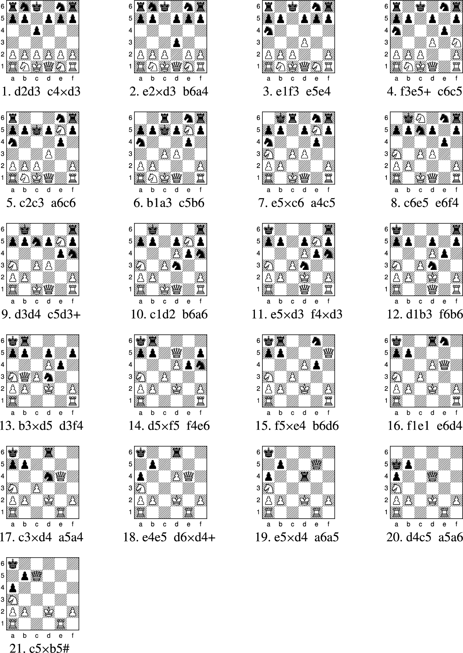
The shape of a DAG (with a single root) can conveniently be described by two histograms, as presented in Table 2, where the first histogram describes the minimum distance from the root within the DAG, and the second histogram describes the maximum distance to a leaf. Conceptually, the first histogram may be thought of a the depth within the proof, where the root appears at depth 1, the 13 positions of Table 1 appear at depth 2 and so on. The second histogram may be consider the mate-in-N number for node, where the root node appears at the bottom of the table, with mate-in-21, and 168,204,805 positions (or 62.94% of the positions) are leaf notes that are mate-in-1. Fig. 7 shows one of the (1446) longest sequences of the proof, also known as a principal variation.

4.Future work

The obvious next goal is to remove the “after P-K3” qualifier, and confirm that there is no opening move for White that avoids defeat. This would require similar proofs to the one given here, for the other ten opening moves. Work on this is already underway.

This proof differs from full 8×8 chess in two important factors; the smaller 6×6 board and the material asymmetry of White playing without a queen. Both dramatically reduce the search space. To determine which factor is more significant, it will be interesting to observe whether solving (symmetric) Los Alamos chess on a 6×6 board, or solving (asymmetric) 8×8 chess without a queen will occur first.

Fig. 7.

The principal variation (longest sequences of moves) of the proof.

5.Conclusion

Advances in computer hardware allow solutions to problems considered impossible just a few years ago. Whilst weakly solving regular chess on an 8×8 board is still some way off, the (weak) solution of a chess-like game on a 6×6 board inevitably brings that day a little bit closer.

6.Supplementary material

A machine-readable file containing the proof, game2_d2d3.proof.gz, is available via figshare as https://figshare.com/articles/dataset/game2_d2d3_proof_gz/25424674. The digital object identifier (DOI) for this file is 10.6084/m9.figshare.25424674. This ASCII text file, contains 267410116 lines, starting with a header comment line (specifying the root position of the proof), followed by one line per position, for each giving the proof move, and for non-mating moves the number moves remaining until checkmate.

References

1 | Allis, V. ((1994) ). Searching for solutions in games and artificial intelligence. PhD thesis, Maastricht University. |
2 | Bell, A.G. ((1978) ). The Machine Plays Chess? Pergamon Press. |
3 | Berliner, H.J. ((1979) ). The B∗ tree search algorithm: A best first proof procedure. Artificial Intelligence, 12: (1), 23–40. doi:10.1016/0004-3702(79)90003-1. |
4 | Berliner, H.J. ((1985) ). Hitech wins North American Computer-Chess Championship. International Computer Games Association (ICGA) Journal, 8: (4), 246–247. doi:10.3233/ICG-1985-8412. |
5 | Breuker, D., Allis, V. & van den Herik, J. ((1994) ). Mate in 38: Applying proof-number search. In J. van den Herik, B. Herschberg and J. Uiterwijk (Eds.), Advances in Computer Chess (Vol. 7: ). |
6 | Campbell, M. & Marsland, T. ((1983) ). A comparison of minimax tree search algorithms. Artificial Intelligence, 20: (4), 347–367. doi:10.1016/0004-3702(83)90001-2. |
7 | Coulom, R. ((2007) ). Efficient selectivity and backup operators in Monte-Carlo tree search. In J. van der Herik, P. Ciancarini and H.H.L.M. Donkers (Eds.), Proceedings Computers and Games. Springer. |
8 | Edwards, S.J. ((1994) ). Standard: Portable game notation specification and implementation guide. https://ia902908.us.archive.org/26/items/pgn-standard-1994-03-12/PGN_standard_1994-03-12.txt. |
9 | Fichter, F. ((2021) ). Fairy-Stockfish. https://fairy-stockfish.github.io/. |
10 | Hyatt, R. & Cozzie, A. ((2005) ). The effect of hash signature collisions in a chess program. International Computer Games Association (ICGA) Journal, 8: (3). |
11 | Kister, J., Stein, P., Ulam, S., Walden, W. & Wells, M. ((1957) ). Experiments in chess. Journal of the ACM, 4: (2), 174–177. doi:10.1145/320868.320877. |
12 | Mhalla, M. & Prost, F. ((2013) ). Gardner’s minichess variant is solved. International Computer Games Association (ICGA) Journal, 36: (4), 215–221. |
13 | Schaeffer, J. ((2008) ). One Jump Ahead: Computer Perfection at Checkers. Springer. |
14 | Shannon, C. ((1950) ). Programming a computer for playing chess. Philosophical Magazine, 41: (314). |
15 | Stein, P. & Ulam, S. ((1957) ). Experiments in chess on electronic computing machines. Chess Review, 13–17. |
16 | Takizawa, H. ((2023) ). Othello is solved, CoRR. doi:10.48550/ARXIV.2310.19387. |
17 | Tromp, J. ((2021) ). Chess position ranking. https://github.com/tromp/ChessPositionRanking. |
18 | Winands, M.H.M., Uiterwijk, J.W.H.M. & van den Herik, H.J. ((2003) ). PDS-PN: A new proof-number search algorithm. Computers and Games, 61–74. doi:10.1007/978-3-540-40031-8_5. |
19 | Zobrist, A. ((1990) ). A new hashing method with application for game playing. International Computer Chess Association (ICCA) Journal, 13: (2). |