
Deep learning based network similarity for model selection
Abstract
Capturing data in the form of networks is becoming an increasingly popular approach for modeling, analyzing and visualising complex phenomena, to understand the important properties of the underlying complex processes. Access to many large-scale network datasets is restricted due to the privacy and security concerns. Also for several applications (such as functional connectivity networks), generating large scale real data is expensive. For these reasons, there is a growing need for advanced mathematical and statistical models (also called generative models) that can account for the structure of these large-scale networks, without having to materialize them in the real world. The objective is to provide a comprehensible description of the network properties and to be able to infer previously unobserved properties. Various models have been developed by researchers, which generate synthetic networks that adhere to the structural properties of real networks. However, the selection of the appropriate generative model for a given real-world network remains an important challenge.
In this paper, we investigate this problem and provide a novel technique (named as TripletFit) for model selection (or network classification) and estimation of structural similarities of the complex networks. The goal of network model selection is to select a generative model that is able to generate a structurally similar synthetic network for a given real-world (target) network. We consider six outstanding generative models as the candidate models. The existing model selection methods mostly suffer from sensitivity to network perturbations, dependency on the size of the networks, and low accuracy. To overcome these limitations, we considered a broad array of network features, with the aim of representing different structural aspects of the network and employed deep learning techniques such as deep triplet network architecture and simple feed-forward network for model selection and estimation of structural similarities of the complex networks. Our proposed method, outperforms existing methods with respect to accuracy, noise-tolerance, and size independence on a number of gold standard data set used in previous studies.
1.Introduction
Datasets emerging from different fields such as biology, neuroscience, engineering, social science, economics, etc. are often represented as networks to understand the complex systems in these fields.
To understand the formation and evolution of real-world networks various generative models have been proposed to generate synthetic networks that follow the non-trivial topological properties of real-world networks [7,13,35,37,57,59]. For example, Watts-Strogatz model [59] synthesizes small-world networks with small average path length and high clustering coefficient, and Barabási–Albert model [7] generate scale-free networks with long-tail (power law) degree distribution. In addition to degree distribution, clustering and path lengths, other structural properties such as modularity, assortativity and special eigenvalues – are also supported in newer generative models [3,35].
Despite the progress made in proposing many generative models, there is currently no universal generative model that is applicable for all applications. Therefore, prior to network generation, we have to perform the non-trivial task of choosing the appropriate generative model for a particular application (also called model selection). Since we want to choose the model that is most representative of the real network, model selection involves deep analysis of the properties of the given network (called target network), and accordingly the most appropriate model is chosen. Essentially, model selection attempts to evaluate a library of candidate generative models and predict which the most appropriate for generating complex network instances similar to the real network. There are many applications of model selection including network sampling [22,34,36,54], simulation of network dynamics [12,42,46] and summarization [2,39,50] etc.
In order to perform effective model selection, we require a similarity measure to compare networks across their topological properties such as average path length, transitivity, clustering coefficient, modularity, etc.. A large amount of existing literature discussed the importance of structural similarity metric for complex networks, an appropriate definition of distance similarity metric is the basis for many machine learning and data analysis tasks such as classification and clustering [10,26,31,40,50]. An important property of the chosen distance metric is that it should be agnostic to network size so that it can compare networks of different scales. This is a departure from other similarity/dissimilarity notions including graph similarity with known node correspondence [31] and classical graph similarity approaches (including graph alignment, graph matching, graph isomorphism) [60,62]. One related approach to developing a network similarity metric is to create a feature vector for each network based on existing network topological properties and then computing the similarity of feature vectors based on Euclidean distance in feature space [10,49,50]. In this paper, we propose a novel method for automatic learning of the similarity metric via a specialized deep neural architecture. The model learns via supervised training wherein it learns from pairs of similar and dissimilar networks and maps the features onto space where distances between similar networks are smaller than distances between dissimilar networks.
2.Related work
In the literature, several network model selection (or network classification) methods are available most of them are based on graphlet counting feature [26,41,48], and combination of local and global features of network topology [2,4,43] for selecting the best generative model. Other methods are also developed for model selection problem [20,27].
To measure the structural similarities between two networks various quantitative measures have been reported [4,10,17,40,48–51,62]. Graph isomorphism is one of the classical approaches to compare two graphs. Two graphs are said to be isomorphic if they have an identical topology. Some variants of this approach are also proposed, including subgraph isomorphism and maximum common subgraphs [11]. Several isomorphism-inspired methods based on counting the number of spanning trees [28] and computing the node-edge similarity scores are also available [62]. These different methods are computationally expensive and not suitable for the large complex networks. Various approaches utilized graphlet counts as a measure of network similarity [26,29,48] and distance measures for network comparison in which network are represented in the form of feature vectors that summarize the network topology [2,11,35,39,50].
In the analysis of complex networks, a size-independent similarity metric plays an important role in the evaluation of the network generation models [7,37,59,60], evaluation of sampling methods [22,34,36,54], study of epidemic dynamics [12,42,46], generative model selection [26,41,43], biological networks comparison [48,49], network classification and clustering [2,16,26,41,43], and anomaly and discontinuity detection [10,45].
3.Materials and methods
In this section we describe our model, formly known as ‘TripleFit’, for complex networks. The model consists of two important processes: (a) model selection and (b) structural network similarity. The model selection is based on the structural similarity between two complex networks. For a given target (realistic) network instance, the proposed method chooses the appropriate generative model among six generative models that can generate a synthetic network similar to the target (realistic) network. The selection of the best model is based on the embedded feature space of the target network and various synthetic networks generated from different generative models. In the proposed method, we developed a network distance metric by utilizing topological features for separating the various types of network classes. The simplest choice would be to compute the Euclidean distance between the two topological feature vectors of two networks. In this way, we utilize the triplet neural network architecture to learn the best distance metric [24]; the goal will be to learn a transformation from the original feature space to an embedded feature space, in which the euclidean distance between similar networks is smaller than distances between dissimilar networks. We also quantify the structural similarity between two networks by computing the Euclidean distance between the corresponding network topological feature vectors in transformed space.
3.1.Dataset description:
In this study, we have taken a gold standard data set 11 named as Reference Networks Datasets (RND) used in the previous study [4] that describes a Noise-tolerant model selection method for complex networks. For evaluating the network model selection they consider six network generative models: Kronecker Graphs (KG) [35], Forest Fire model (FF) [37], Barabási-Albert model (BA) [7], Watts-Strogatz model (WS) [59], Erdös-Rényi (ER) [19] and Random Power Law (RP) [57]. The detailed description of the dataset is given in the referred study [4].
Fig. 1.
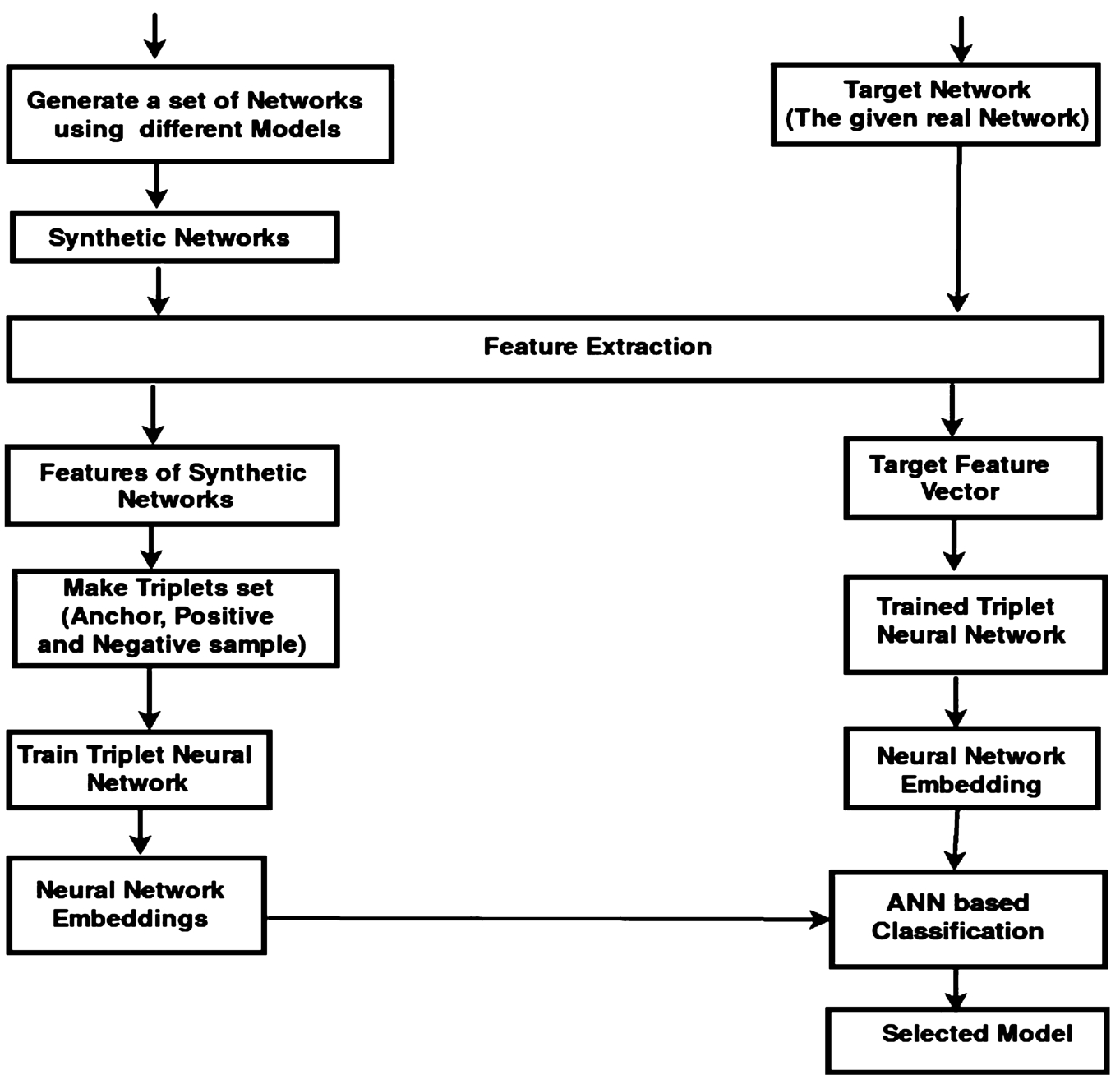
The proposed methodology for model selection.
3.2.Overall model selection strategy
Figure 1 shows a high-level view of the model selection process. The methodology is configurable by several decision points, such as the set of considered network features, the candidate generative models. The steps for constructing the final network classifier are described here:
(1) We took 1000 network instances of different size and densities (using different parameters) for each candidate network generative model from RND, for capturing their growth mechanism and generation process. These network instances will form the dataset for learning the triplet neural network.
(2) We extract the topological features (clustering coefficient, modularity, degree distribution, etc.) of each network instance. The result is a dataset of labeled structural features in which each record consists of topological features of a synthesized network along with the label of its generative model.
(3) Construct the triplets a from the labeled dataset which comprises of the positive, negative and anchor samples, where the positive and anchor sample is of the same class (or same generative model), and the negative sample is of a different class. These triplets are utilized for learning the distance metric using a triplet network. So, we train the triplet neural network using the different triplets. This trained triplet neural network transforms the feature space into another feature space (called embedding feature space) in which the distance between the positive and anchor sample is smaller than the distance between negative and anchor sample. This new embedding feature space will form the dataset for learning a network classifier.
(4) The labeled embedding feature dataset forms the training and test data for a supervised learning algorithm. The learning algorithm will return a network classifier which can predict the class (the best generative model) for a given network instance.
(5) The same topological features used in Step 2 are also extracted from the real world (target) network. Then pass this feature vector into trained triplet neural network, which we trained in Step 3 and generate the embedding feature vector of the target network. This embedding feature vector of the target network is used as the input of the learned classifier, which is trained in Step 4.
The learned network classifier is a customized model selector for finding the model that fits the target network. It gets the topological features of the target network as the input and returns the most compatible generative model.
Besides the network model selection, proposed method also estimate the structural similarities of networks. For measuring the structural similarity between two networks, we extract the topological features of two given networks as in Step 2. Then we pass both feature vectors into trained triplet neural network, trained in Step 3, and generate embedding feature vectors for both networks. Then we compute the Euclidean distance between the two embedding feature vectors, representing the similarity between two networks. The distances between similar networks are smaller compared to dissimilar networks. Section 4.3 describes the computation of structural similarities between the network instances generated in Step 1. Detailed description of the steps described in the above section are presented below:
3.3.Network features
The process of model selection, as described in Fig. 1, utilizes network topological features in the second and fifth steps. There are various features are defined in network literature to quantify the topological properties of the network. We considered only some well-known and frequently studied measures, which are relevant to our study. A diverse set of local and global network features were utilized to construct feature vectors. A brief description of the calculated measures is as follows:
Degree distribution: Degree distribution defined as the probability distribution of the degrees of all nodes of the network. We quantify a degree distribution by computing its variance
Where
Entropy: The entropy of the degree distribution provides an average measurement of the heterogeneity which in turn determines the robustness of the network. Formally, the entropy is defined as [16]:
WhereClustering coefficient: Clustering coefficient is a measure of segregation in network analysis. Clustering coefficient
The clustering coefficient C for the whole network is calculated by the average value ofCharacteristic path length: The mean of the shortest path length between all pairs of nodes also called the characteristic path length [59] and is a measure of network integration. For a graph G with n nodes, the network characteristic path length is given by:
whereEfficiency: Global efficiency is a measure of integration, that is the calculated by average inverse shortest path length between all pairs of nodes in the network. For a graph G with n nodes and k edges, the global efficiency of a network is defined as [1,33]:
whereAssortativity coefficient: Assortativity is a measure of how well nodes of similar degree are linked to one another in the network. A network is said to show assortative mixing if high degree nodes have a high tendency to connect to other high degree nodes and similarly low degree nodes have a bias towards connecting to low degree nodes. To quantify the level of assortative mixing in a network we define an assortativity coefficient which is defined as [44]:
Where
Modularity: Modularity has been widely used as a quality measure for measure the strength of division of a network into modules (also called cluster or communities). Networks with high modularity have dense connections between the nodes within modules but sparse connections between nodes in different modules. The modularity of an unweighted graph partitioned into modules is evaluated by [15]:
Where
Network features are not standardized i.e. there is no universal best set of features for networks and other features such as shrinking diameter, densification, vulnerability, network resilience, rich-club phenomenon, etc. have also been used. The proposed methodology is not limited to the specified network feature set. Hence, one can also utilize another set of features, according to their application domain. In this study, we utilized only 8 network topological features.
3.4.Triplet neural network
Triplet neural network is a deep learning model, which aims to learn useful representations of data by distance comparisons [24]. Recently, triplet network architecture have successfully applied in many computer vision tasks [14,32,52,58]. In past few years, deep learning models have been widely exploited to solve various machine learning tasks. Deep Learning is automating the extraction of high-level meaningful complex abstractions as data representations (features) through the use of a hierarchical learning approach. The notion of hierarchical features stems from neuroscientific discoveries of the visual cortex that indicate a hierarchy of cells with successively higher level cells firing for more complex visual patterns [5,8,9,23,61].
Fig. 2.
A schematic representation of triplet neural network architecture, which consists three feed forward neural networks of the same instance with shared parameters.
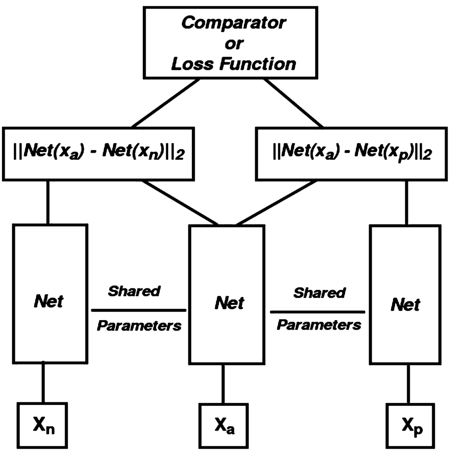
Triplet network, as shown in the Fig. 2, is a model inspired by the Siamese Network which comprise three feed forward networks of the same instance with shared parameters. The network gives two intermediate values when fed three samples to it. These intermediate values come from
We train this network for a 2-class classification problem using the triplet input
3.5.Triplet neural network architecture
Here, we briefly describe the implementation details of Triplet Neural Network. A Triplet Neural Network consists of three feedforward neural networks of shared weights, followed by two layers. An advanced activation function ELU (Exponential Linear Unit) are applied between two consecutive layers. Network configuration (ordered from input to output) consists of layers dimensions
3.6.Network models
Among several existing network generative models, we have selected six important models: Kronecker Graphs (KG) [35], Forest Fire model (FF) [37], Barabási-Albert model (BA) [7], Watts-Strogatz model (WS) [59], Erdös-Rényi (ER) [19] and Random Power Law (RP) [57]. The selected models are the state of the art methods of network generation. Existing model selection methods have ignored some new and important generative models such as Kroneckr graphs and Forest Fire [4]. All the models are briefly described in the study [4]. The characteristic of above six generative models are defined as follows:
Erdös-Rényi (ER): This model generates completely random networks. The number of nodes and edges are configurable [19].
Barabási-Albert model (BA): This model generates random scale-free networks using a preferential attachment mechanism [7].
Watts-Strogatz model (WS): This model generates synthetic networks with small characteristic path lengths and high clustering coefficient. It starts with a regular lattice and then rewires some edges of the network randomly [59].
Forest Fire model (FF): In this model, edges are added in a process similar to a fire-spreading process. This model is inspired by Copying model and Community Guided Attachment but supports the shrinking diameter property [37].
Random Power Law Model (RP): The RP model generates synthetic networks by following a variation of ER model that supports the power law degree distribution property [57].
Kronecker Graphs (KG): This model generates realistic synthetic networks by applying a non standard matrix operation (the kronecker product) on a small initiator matrix. This model is mathematically tractable and supports many network features, such as heavy tail degree distribution, small diameters, heavy tails for eigenvalues and eigenvectors, and densification and shrinking diameters over time [35].
4.Results
In this section, we evaluate our proposed method for network model selection and structural network similarity. We utilize the RND to evaluate our model against other existing methods. The proposed model is evaluated by first transforming the networks dataset into the feature dataset using the topological features mentioned in Section 3.3. Thus we have several network instances generated using six generative models and many real world networks that correspond to one feature vector representation in feature dataset. In previous methods size (number of nodes) and/or density of a target network is considered in the generation of training data [26,41,43]. In our methodology, the size and density of the target network are not considered in the generation of the training data. In the proposed method, a Triplet Neural Network is utilized to find the best network distance metric, which is capable of separating networks of different classes.
4.1.Evaluation of network distance metric
The TripletFit method is primarily based on learning of network distance metric. The distance metric learning problem is concerned with learning a distance function, which can separate networks of different generative models. In this study, we choose euclidean distance (
Fig. 3.
Visualization of embedded feature set into two dimensional space using t-SNE method.
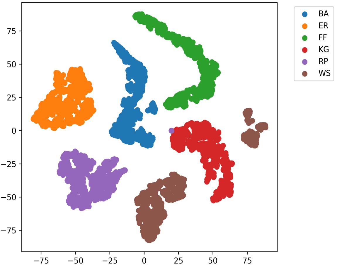
In this section, we show that learned distance function is capable of separating different class generative models. In this order, we visualize the high-dimensional embedded feature dataset using T-Distributed Stochastic Neighbor Embedding (t-SNE) technique, which projects the high-dimensional embedding data into low dimensional embedding. t-SNE is a non-linear dimensionality reduction technique, allowing visualize of high-dimensional data. It learned the low dimensional embedding by minimizing the Kullback-Leibler divergence between the two distributions: a distribution that measures pairwise similarities of the input data points and a distribution that measures pairwise similarities of the corresponding low-dimensional points in the embedding [55,56]. t-SNE representation of high-dimensional embedded features dataset into two-dimensional space is given in Fig. 3, where different colors are shown, different generative models.
As described in Fig. 3, each class of generative model is clearly separate in embedding feature space. Hence, we utilized the embedded feature dataset for both model selection (network classification) and network similarities (network comparison).
4.2.Evaluation of the model selection approach
First, we evaluate the TripletFit for model selection, on the synthetic labeled dataset, which is constructed by the network instances of known generative models mentioned in Section 3.6. To the best of our knowledge, these are the most widely used generative models in network generation applications, and they also cover a wide range of network structures.
Each generative model offers a set of parameters for tuning the synthesized networks so that they follow the properties of real (target) networks. The Number of nodes (or network size) is an important parameter of considered models. Unlike other network model selection methods [2,26,41,43,48], we select the all the parameters randomly. The size of the network is randomly chosen from 1000 to 5000 nodes, and other network parameters are also chosen randomly from the parameter ranges described in study [4]. As compared with the size of real (target) network, we generate smaller sizes of the network instances for training the proposed method. This feature increases the efficiency and performance of our proposed method.
The generative model selection is treated as a network classification problem. In this study, we developed a supervised learning algorithm for network model selection. In this way, we utilized an Artificial Neural Network (ANN) model [25,30] as a classifier to select an appropriate generative model for a given real network. For training the ANN model, we utilized embedded features dataset generated in Step 3 of Section 3.2. We performed 10-fold cross-validation process for evaluation of our proposed method, where the whole dataset is randomly divided into 10 equal subsets. From the 10 subsets, a single subset is retained as a test set, and the remaining subsets are used as a training data. This process repeated 10 times. We construct the test set in such a way that, every iteration contained an equal number of networks instances (i.e., 100) of each generative model. The final accuracy of proposed method is calculated by mean of accuracies of each iteration. The detailed average results (average outcome of 10-folds) of the classifier is given in Table 1.
Table 1
Results of TripletFit method on synthetic network dataset
| Pred | True | ||||||
| BA | ER | FF | KG | RP | SW | Class precision | |
| BA | 100 | 0 | 0 | 0 | 0 | 0 | 100% |
| ER | 0 | 100 | 0 | 0 | 0 | 0 | 100% |
| FF | 0 | 0 | 100 | 0 | 0 | 0 | 100% |
| KG | 0 | 0 | 0 | 100 | 2 | 0 | 98.04% |
| RP | 0 | 0 | 0 | 0 | 98 | 0 | 100% |
| SW | 0 | 0 | 0 | 0 | 0 | 100 | 100% |
| Class recall | 100% | 100% | 100% | 100% | 98% | 100% | Accuracy: 99.70 % |
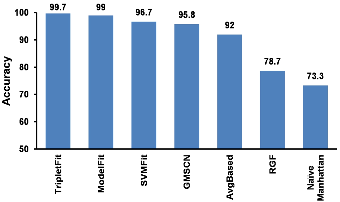
Aliakbary et al. [4] compared their proposed method (ModelFit) with various existing model selection methods: GMSCN [43], SVMFit [30,47], RGF [49], AvgBased, Naïve-Manhattan. GMSCN utilized LADTree decision tree classifier on RND. SVMFit is an SVM-based classification method. AvgBased is a distance based classifier which considers an average distance of the given network with neighbor networks. RGF-method is another distance based method, utilizes the concept of the graphlet count features. Finally, the Naïve-Manhattan distance can be defined as pure Manhattan distance of the network features, where all the network features shares the equal weights during distance calculation. More details about these methods can be found through the research paper [4]. We compared our proposed method with other methods reported in the work of Aliakbary et al. [4], a comparative summary of results is shown in Fig. 4.
Fig. 4.
The accuracy comparison of different network selection methods.
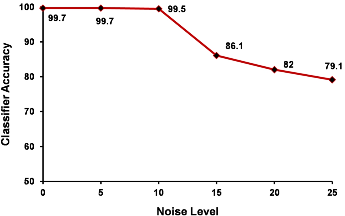
We also evaluate the robustness of our proposed method by introduce varying noise levels (noise =
Fig. 5.
The robustness of TripleFit with respect to different levels of noise.
4.3.Evaluation of the network similarity approach
In this section, we measure the structural similarities between different synthetic and real world complex networks. In order to measure the structural network similarity between two networks, we compute the euclidean distance between the embedded feature vectors of corresponding networks.
Fig. 6.
Structural similarities between synthetic networks.
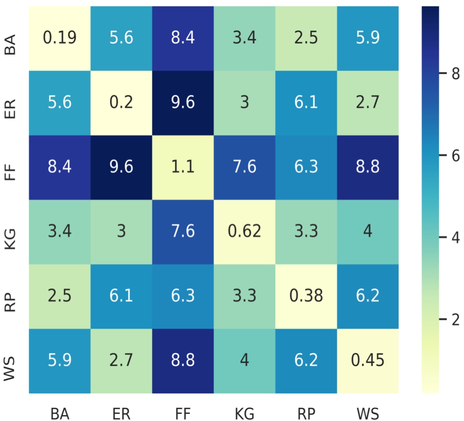
We employ the Euclidean distance as a structural network similarity measure for comparison of real networks. To measures the structural similarity between two networks, compute euclidean distance between embedded features of these two networks. The question: is the euclidean distance capable of describing the structural similarities in real network data? In order to evaluate this, we compute the euclidean distance between every pair of embedded feature vectors of 6000 network instances, generated by six different generative models as described in Step 4 of Section 3.2. Then we plot a heatmap of this
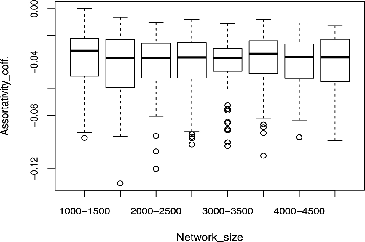
4.4.Effect of network sizes on assortativity measure
The assortativity coefficient has been shown dependency upon network size [38]. Hence, we carried out an extensive analysis of this issue. In the Appendix: Figs 7 to 12 shows the boxplots of assortativity in various network size ranges for different network types. We do confirm that a few network types, particularly the Barabási-Albert model, assortativity slightly increases with network size. The major implication of this observation is that the proposed approach should not be used for a very large range of network sizes. It is to be noted that the dependencies are rather weak, with a reasonable range of network sizes, hence the proposed model can be used effectively as has been demonstrated in our study. Further, we carried out an additional experiment in which we removed the assortativity feature from our model and the results shows that this feature is not critical to the overall strategy of the proposed network comparison methodology. Thus, if users intend to reuse our model for a very large range of network sizes, they are advised to remove assortativity features and the cost of doing so in terms of model performance is not very high.
4.5.Case study
In order to find the effectiveness of proposed method for real networks, we have applied TripleFit on some real networks. The real network instances and the results of TripletFit on these networks are described below:
(1) “p2p-Gnutella08”, Gnutella is a small peer to peer file sharing network with about
(2) “Email-URV”, Email-URV is the network of emails interchanges between members of the University Rovira i Virgili of Tarragona, Spain. This data set is collected by Guimera et al. [21]. The data covers total
(3) “email-Enron”, email-Enron is the communication network covers all the email communication of Federal Energy Regulatory Commission during its investigation. In this network nodes represent the email addresses and an edge represents the email interchange between two address i.e., an address sent at least one email to other address.
(4) “cit-HepPh”, cit-HepPh is a arxiv High Energy Physics Phenomenology paper citation network. Which covers all the citations within a dataset of
(5) “cit-HepTh” cit-HepTh is a arxiv High Energy Physics Theory paper citation network. Which covers all the citations within a dataset of
(6) “ca-HepPh” ca-HepPh is a arxiv High Energy Physics Phenomenology collaboration network (or co-authorship network). Which covers scientific collaborations between authors papers submitted to High Energy Physics – Phenomenology category within a dataset of
(7) “ca-HepTh” ca-HepPh is a arxiv High Energy Physics Theory collaboration network (or co-authorship network). Which covers scientific collaborations between authors papers submitted to High Energy Physics – Theory category within a dataset of
Table 2 shows the results after applying Tripletfit on the real networks as described above. As Table 2 shows, various real-networks, which are selected from a wide range of sizes, densities and domains, are categorized in different network models by the classifier. This fact indicates that no generative model is dominated in proposed method for real networks and it suggests different models for different network structures. The case study also verifies that no generative model is sufficient for synthesizing networks similar to real networks and we should find the best model fitting the target network in each application. As a result, the task of generative model selection is an important stage before generating network instances. Accordingly for the chosen seven real networks the appropriate generative model selected and shown in last column of Table 2.
Table 2
Real networks and the selected generative model using network model selection method
| Network | No. of nodes | No. of edges | Selected model |
| p2p-Gnutella08 [53] | 6301 | 20777 | SW |
| Email-URV [18] | 1133 | 10903 | FF |
| email-Enron [53] | 36692 | 367662 | SW |
| cit-HepPh [53] | 34546 | 421578 | BA |
| cit-HepTh [53] | 27770 | 352807 | FF |
| ca-HepPh [53] | 12008 | 237010 | SW |
| ca-HepTh [53] | 9877 | 51971 | BA |
As we discussed, we can utilize network similarity method for model selection. So in that way we compute euclidean distance between embedded features of real networks and generative networks (synthesized by generative network models). Table 3 shows the average euclidean distance between embedded features of a real network and all instances of particular generative network. A smallest average distance shows strong structural similarity between real network and generative network.
Table 3
Real networks and the selected generative model using structural network similarity method
| Real networks | Generative networks | ||||||
| BA | ER | FF | KG | RP | SW | Selected model | |
| p2p-Gnutella08 [53] | 44.94 | 40.43 | 30.71 | 44.75 | 44.92 | 30.21 | SW |
| Email-URV [18] | 18.29 | 13.78 | 3.56 | 18.10 | 18.28 | 4.06 | FF |
| email-Enron [53] | 87.8 | 83.3 | 73.57 | 87.61 | 87.79 | 73.07 | SW |
| cit-HepPh [53] | 0.21 | 4.29 | 14.51 | 0.32 | 0.29 | 14.01 | BA |
| cit-HepTh [53] | 16.4 | 11.9 | 1.72 | 16.22 | 16.4 | 2.18 | FF |
| ca-HepPh [53] | 72.85 | 68.35 | 58.63 | 72.67 | 72.86 | 58.12 | SW |
| ca-HepTh [53] | 0.31 | 4.19 | 14.42 | 0.39 | 0.34 | 13.92 | BA |
5.Discussion
In this paper, we proposed a novel method for network model selection and network similarity. In this method, we investigated the network distance metric for comparing the topological propoerties (topology) of the complex networks. In simple words for a given real network find the matching generative model using network topology based features. The computational strategy adopted include first generating instances from select group of generative models. Second the triplet set of features characterizing the network property from the above set of instances and thirdly these features are embedded and fed as input to the classifier and the other input to the classifier come from the real network data refer Fig. 1. The classifier will provide us to appropriate generative model that fits real network. The second objective is to estimate the network similarity using euclidean distance measure. The result of our analysis with seven real networks shows the usefulness of proposed method refer Tables 2 and 3. We have seen in our study that the model selected through model selection (using classification scheme) and the model selected through network similarity (using euclidean distance measure) agreed completely refer Tables 2 and 3.
Figure 5 shown the sensitiveness of proposed method to perturbations in the network topology by introducing various noise levels (or variability i.e. noise = 5%, 10%, 15%, 20%, 25%) into test case network. The noise was introduced in the network by rewiring a particular fraction of network edges between the randomly selected pair of nodes. We observe that the classification performance of proposed methodology do not affected upto 10% of noise after that it drops considerably. In other words the proposed method is less sensitive to perturbation in network topology of test set. Hence it is independent of size and density of the test case network (e.g., a real network). Therefore, variability factor is considered clearly in proposed methodology.
In our methodology, the size and density of the target network are not considered in the generation of the training data. Size and density independence is an important feature of our method. It enables the classifier to learn from a dataset of generated networks with different sizes and different densities, perhaps smaller than the size of the target network. For example, given a very large size of network instance as the target network, we can prepare the dataset of generated networks with smaller size than the target network. This facility decreases the time of network generation and feature extraction considerably. The proposed method outperforms the various existing methods, which highlight the effectiveness of deep learning architectures in the learning of a distance metric for topological comparison of complex networks. Our proposed method (TripletFit), outperforms the state-of-the-art methods with respect to accuracy and noise tolerance.
Benefits of our study may help biologist to mimic real word network this may help further insight into the network topology and properties. With the large scale generation of Next Gen Sequencing data and its annotation may further demand fast and reliable model selection software tools. The present study may in the direction too.
Author contributions
K.V.S. and L.V. conceived and designed the study. K.V.S. and A.K.V. implemented the algorithm and prepared the figures of the numerical results. K.V.S., A.K.V. and L.V. analyzed and interpreted the results, and wrote the manuscript. All the authors have read and approved the final manuscript.
Competing interests
We declare that there is no competing of interests for this work.
Notes
1 Downloaded from http://ce.sharif.edu/~aliakbary/datasets.html on May 5, 2016.
Acknowledgements
The authors would like to thank J.N.U. and U.G.C., India for providing the research fellowship to K.V.S. and A.K.V.
Appendices
Appendix
AppendixAssortative plots for different network size
In this section, we describe the boxplots of assortativity in various network size ranges under different network types.
Fig. 7.
Assortativity boxplot for Barabási-Albert model.
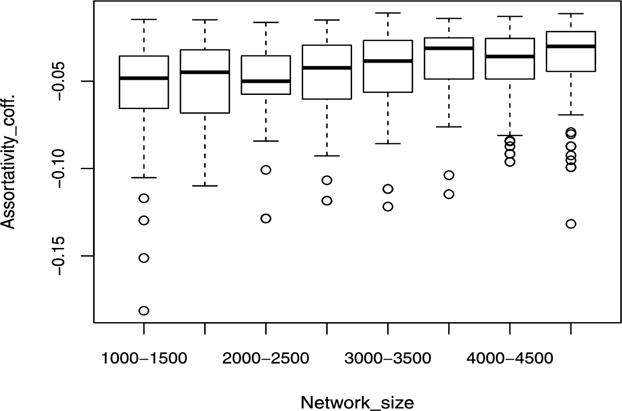
Fig. 8.
Assortativity boxplot for Erdös-Rényi model.
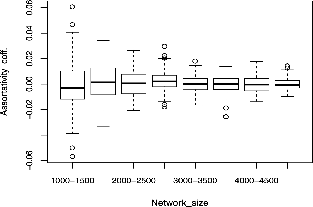
Fig. 9.
Assortativity boxplot for forest fire model.
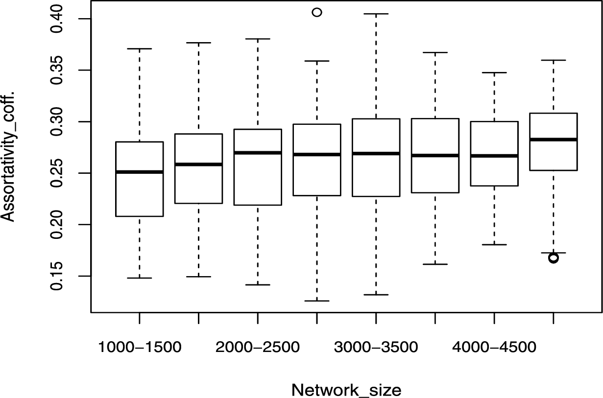
Fig. 10.
Assortativity boxplot for Kronecker graphs.
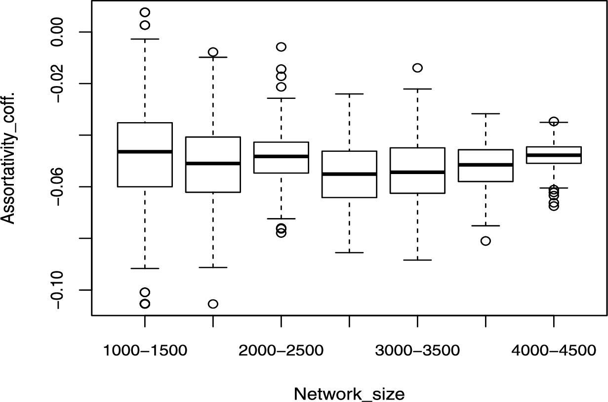
Fig. 11.
Assortativity boxplot for random power law model.
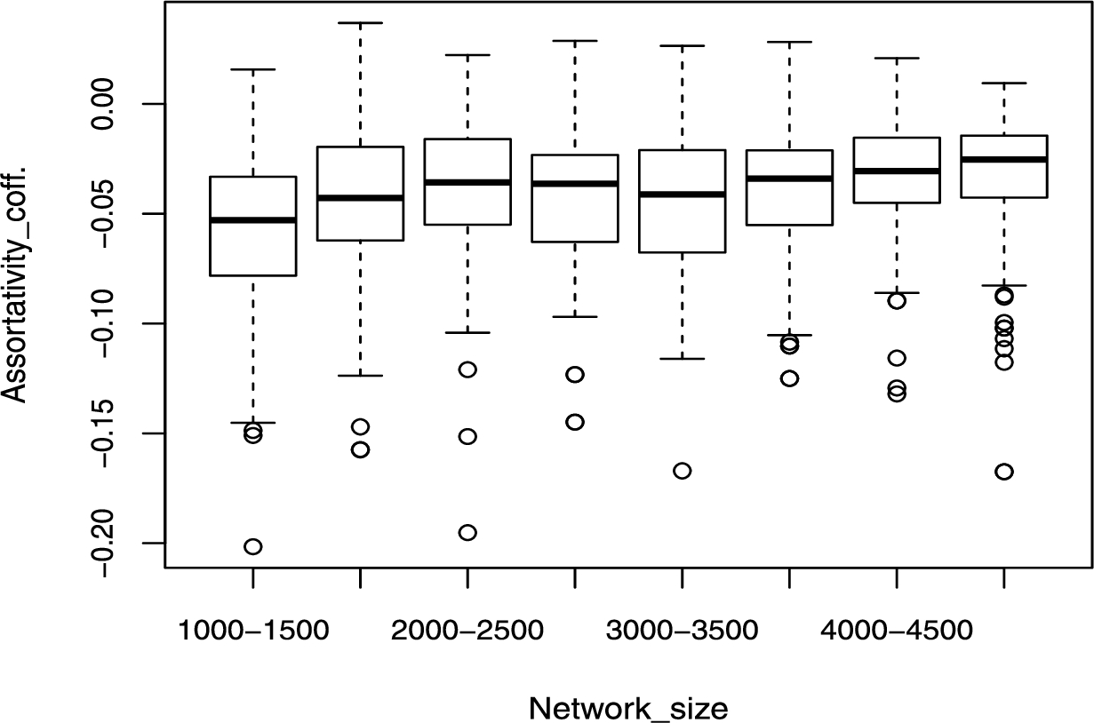
Fig. 12.
Assortativity boxplot for Watts-Strogatz model.
References
[1] | S. Achard and E. Bullmore, Efficiency and cost of economical brain functional networks, PLoS Comput Biol 3: (2) ((2007) ), e17. |
[2] | E.M. Airoldi, X. Bai and K.M. Carley, Network sampling and classification: An investigation of network model representations, Decision support systems 51: (3) ((2011) ), 506–518. doi:10.1016/j.dss.2011.02.014. |
[3] | L. Akoglu and C. Faloutsos, RTG: A recursive realistic graph generator using random typing, in: Joint European Conference on Machine Learning and Knowledge Discovery in Databases, Springer, Berlin Heidelberg, (2009) , pp. 13–28. doi:10.1007/978-3-642-04180-8_13. |
[4] | S. Aliakbary, S. Motallebi, S. Rashidian, J. Habibi and A. Movaghar, Noise-tolerant model selection and parameter estimation for complex networks, Physica A: Statistical Mechanics and its Applications 427: ((2015) ), 100–112. doi:10.1016/j.physa.2015.02.032. |
[5] | I. Arel, D.C. Rose and T.P. Karnowski, Deep machine learning – a new frontier in artificial intelligence research [research frontier], IEEE Computational Intelligence Magazine 5: (4) ((2010) ), 13–18. doi:10.1109/MCI.2010.938364. |
[6] | J.M. Badham, Commentary: Measuring the shape of degree distributions, Network Sci. 1: ((2013) ), 213–225. doi:10.1017/nws.2013.10. |
[7] | A.-L. Barabási and R. Albert, Emergence of scaling in random networks, Science 286: (5439) ((1999) ), 509–512. doi:10.1126/science.286.5439.509. |
[8] | Y. Bengio, A. Courville and P. Vincent, Representation learning: A review and new perspectives, IEEE transactions on pattern analysis and machine intelligence 35: (8) ((2013) ), 1798–1828. doi:10.1109/TPAMI.2013.50. |
[9] | Y. Bengio and Y. LeCun, Scaling learning algorithms towards AI, Large-scale kernel machines 34: (5) ((2007) ), 1–41. |
[10] | M. Berlingerio, D. Koutra, T. Eliassi-Rad and C. Faloutsos, Network similarity via multiple social theories, in: Advances in Social Networks Analysis and Mining (ASONAM), 2013 IEEE/ACM International Conference on, IEEE, (2013) , pp. 1439–1440. |
[11] | Borgwardt and K. Michael, Graph kernels, 2007, PhD diss. |
[12] | L. Briesemeister, P. Lincoln and P. Porras, Epidemic profiles and defense of scale-free networks, in: Proceedings of the 2003 ACM Workshop on Rapid Malcode, ACM, (2003) , pp. 67–75. doi:10.1145/948187.948200. |
[13] | D. Chakrabarti and C. Faloutsos, Graph mining: Laws, generators, and algorithms, ACM computing surveys (CSUR) 38: (1) ((2006) ), 2. doi:10.1145/1132952.1132954. |
[14] | G. Chechik, V. Sharma, U. Shalit and S. Bengio, Large scale online learning of image similarity through ranking, Journal of Machine Learning Research 11: ((2010) ), 1109–1135. |
[15] | A. Clauset, M.E. Newman and C. Moore, Finding community structure in very large networks, Physical review E 70: (6) ((2004) ), 066111. doi:10.1103/PhysRevE.70.066111. |
[16] | Costa, L.da F., F.A. Rodrigues, G. Travieso and P. Ribeiro Villas Boas, Characterization of complex networks: A survey of measurements, Advances in physics 56: (1) ((2007) ), 167–242. doi:10.1080/00018730601170527. |
[17] | B. Crawford, R. Gera, J. House, T. Knuth and R. Miller, Graph structure similarity using spectral graph theory, in: International Workshop on Complex Networks and Their Applications, Springer International Publishing, (2016) , pp. 209–221. |
[18] | E-mail network URV, Retrieved from http://deim.urv.cat/~alexandre.arenas/data/welcome.htm on January 16, 2017. |
[19] | P. Erdös and A. Rényi, On the central limit theorem for samples from a finite population, Publ. Math. Inst. Hungar. Acad. Sci 4: ((1959) ), 49–61. |
[20] | Goncalves, W. Nunes, A. Souto Martinez and O. Martinez Bruno, Complex network classification using partially self-avoiding deterministic walks, Chaos: An Interdisciplinary Journal of Nonlinear Science 22: (3) ((2012) ), 033139. doi:10.1063/1.4737515. |
[21] | R. Guimera, L. Danon, A. Diaz-Guilera, F. Giralt and A. Arenas, Self-similar community structure in a network of human interactions, Physical review E 68: (6) ((2003) ), 065103. doi:10.1103/PhysRevE.68.065103. |
[22] | J.-D.J. Han, D. Dupuy, N. Bertin, M.E. Cusick and M. Vidal, Effect of sampling on topology predictions of protein-protein interaction networks, Nature biotechnology 23: (7) ((2005) ), 839–844. doi:10.1038/nbt1116. |
[23] | G.E. Hinton, Learning multiple layers of representation, Trends in cognitive sciences 11: (10) ((2007) ), 428–434. doi:10.1016/j.tics.2007.09.004. |
[24] | E. Hoffer and N. Ailon, Deep metric learning using triplet network, in: International Workshop on Similarity-Based Pattern Recognition, Springer International Publishing, (2015) , pp. 84–92. doi:10.1007/978-3-319-24261-3_7. |
[25] | K. Hornik, M. Stinchcombe and H. White, Multilayer feedforward networks are universal approximators, Neural networks 2: (5) ((1989) ), 359–366. doi:10.1016/0893-6080(89)90020-8. |
[26] | J. Janssen, M. Hurshman and N. Kalyaniwalla, Model selection for social networks using graphlets, Internet Mathematics 8: (4) ((2012) ), 338–363. doi:10.1080/15427951.2012.671149. |
[27] | G. Jurman, R. Visintainer, M. Filosi, S. Riccadonna and C. Furlanello, The HIM glocal metric and kernel for network comparison and classification, in: IEEE International Conference on Data Science and Advanced Analytics (DSAA), IEEE, (2015) , p. 1–10. |
[28] | A.K. Kelmans, Comparison of graphs by their number of spanning trees, Discrete Mathematics 16: (3) ((1976) ), 241–261. doi:10.1016/0012-365X(76)90102-3. |
[29] | R. Kondor, N. Shervashidze and K.M. Borgwardt, The graphlet spectrum, in: Proceedings of the 26th Annual International Conference on Machine Learning, ACM, (2009) , pp. 529–536. |
[30] | S.B. Kotsiantis, I. Zaharakis and P. Pintelas, Supervised machine learning: A review of classification techniques, 2007, pp. 3–24. |
[31] | D. Koutra, J.T. Vogelstein and C. Faloutsos, Deltacon: A principled massive-graph similarity function, in: Proceedings of the 2013 SIAM International Conference on Data Mining, Society for Industrial and Applied Mathematics, (2013) , pp. 162–170. |
[32] | B.G. Kumar, G. Carneiro and I. Reid, Learning local image descriptors with deep Siamese and triplet convolutional networks by minimising global loss functions, in: Proceedings of the IEEE Conference on Computer Vision and Pattern Recognition, (2016) , pp. 5385–5394. |
[33] | V. Latora and M. Marchiori, Efficient behavior of small-world networks, Physical review letters 87: (19) ((2001) ), 198701. doi:10.1103/PhysRevLett.87.198701. |
[34] | Lee, S. Hoon, P.-J. Kim and H. Jeong, Statistical properties of sampled networks, Physical Review E 73: (1) ((2006) ), 016102. doi:10.1103/PhysRevE.73.016102. |
[35] | J. Leskovec, D. Chakrabarti, J. Kleinberg, C. Faloutsos and Z. Ghahramani, Kronecker graphs: An approach to modeling networks, Journal of Machine Learning Research 11: ((2010) ), 985–1042. |
[36] | J. Leskovec and C. Faloutsos, Sampling from large graphs, in: Proceedings of the 12th ACM SIGKDD International Conference on Knowledge Discovery and Data Mining, ACM, (2006) , pp. 631–636. doi:10.1145/1150402.1150479. |
[37] | J. Leskovec, J. Kleinberg and C. Faloutsos, Graphs over time: Densification laws, shrinking diameters and possible explanations, in: Proceedings of the Eleventh ACM SIGKDD International Conference on Knowledge Discovery in Data Mining, ACM, (2005) , pp. 177–187. doi:10.1145/1081870.1081893. |
[38] | N. Litvak and R. Van Der Hofstad, Uncovering disassortativity in large scale-free networks, Physical Review E 87: (2) ((2013) ), 022801. doi:10.1103/PhysRevE.87.022801. |
[39] | P. Mahadevan, D. Krioukov, K. Fall and A. Vahdat, Systematic topology analysis and generation using degree correlations, in: In ACM SIGCOMM Computer Communication Review, Vol. 36: , ACM, (2006) , pp. 135–146. |
[40] | A. Mehler, Structural similarities of complex networks: A computational model by example of wiki graphs, Applied Artificial Intelligence 22: (7–8) ((2008) ), 619–683. doi:10.1080/08839510802164085. |
[41] | M. Middendorf, E. Ziv and C.H. Wiggins, Inferring network mechanisms: The Drosophila melanogaster protein interaction network, Proceedings of the National Academy of Sciences of the United States of America 102: (9) ((2005) ), 3192–3197. doi:10.1073/pnas.0409515102. |
[42] | A. Montanari and A. Saberi, The spread of innovations in social networks, Proceedings of the National Academy of Sciences 107: (47) ((2010) ), 20196–20201. doi:10.1073/pnas.1004098107. |
[43] | S. Motallebi, S. Aliakbary and J. Habibi, Generative model selection using a scalable and size-independent complex network classifier, Chaos: An Interdisciplinary Journal of Nonlinear Science 23: (4) ((2013) ), 043127. doi:10.1063/1.4840235. |
[44] | M.E.J. Newman, Assortative mixing in networks, Physical review letters 89: (20) ((2002) ), 208701. doi:10.1103/PhysRevLett.89.208701. |
[45] | P. Papadimitriou, A. Dasdan and H. Garcia-Molina, Web graph similarity for anomaly detection, Journal of Internet Services and Applications 1: (1) ((2010) ), 19–30. doi:10.1007/s13174-010-0003-x. |
[46] | R. Pastor-Satorras and A. Vespignani, Epidemic dynamics in finite size scale-free networks, Physical Review E 65: (3) ((2002) ), 035108. doi:10.1103/PhysRevE.65.035108. |
[47] | J.C. Platt, Fast training of support vector machines using sequential minimal optimization, in: Advances in Kernel Methods, MIT Press, (1999) , pp. 185–208. |
[48] | N. Pržulj, Biological network comparison using graphlet degree distribution, Bioinformatics 23: (2) ((2007) ), e177–e183. |
[49] | N. Pržulj, D.G. Corneil and I. Jurisica, Modeling interactome: Scale-free or geometric?, Bioinformatics 20: (18) ((2004) ), 3508–3515. doi:10.1093/bioinformatics/bth436. |
[50] | A. Sala, L. Cao, C. Wilson, R. Zablit, H. Zheng and Y. Ben Zhao, Measurement-calibrated graph models for social network experiments, in: Proceedings of the 19th International Conference on World Wide Web, ACM, (2010) , pp. 861–870. doi:10.1145/1772690.1772778. |
[51] | T.A. Schieber, L. Carpi, A. Díaz-Guilera, P.M. Pardalos, C. Masoller and M.G. Ravetti, Quantification of network structural dissimilarities, Nature communications 8: ((2017) ), 13928. doi:10.1038/ncomms13928. |
[52] | F. Schroff, D. Kalenichenko and J. Philbin, Facenet: A unified embedding for face recognition and clustering, in: Proceedings of the IEEE Conference on Computer Vision and Pattern Recognition, (2015) , pp. 815–823. |
[53] | SNAP: Stanford Network Analysis Project, Retrieved from http://snap.stanford.edu/ on January 16, 2017. |
[54] | Stumpf, P.H. Michael and C. Wiuf, Sampling properties of random graphs: The degree distribution, Physical Review E 72: (3) ((2005) ), 036118. doi:10.1103/PhysRevE.72.036118. |
[55] | L. van der Maaten and G. Hinton, Visualizing data using t-SNE, Journal of Machine Learning Research 9: ((2008) ), 2579–2605. |
[56] | L.J.P. van der Maaten, Learning a parametric embedding by preserving local structure, in: Proceedings of the Twelfth International Conference on Artificial Intelligence and Statistics (AIS-TATS), JMLR W&CP, Vol. 5: , (2009) , 384–391. |
[57] | D. Volchenkov and P. Blanchard, An algorithm generating random graphs with power law degree distributions, Physica A: Statistical Mechanics and its Applications 315: (3) ((2002) ), 677–690. doi:10.1016/S0378-4371(02)01004-X. |
[58] | J. Wang, Y. Song, T. Leung, C. Rosenberg, J. Wang, J. Philbin, B. Chen and Y. Wu, Learning fine-grained image similarity with deep ranking, in: Proceedings of the IEEE Conference on Computer Vision and Pattern Recognition, (2014) , pp. 1386–1393. |
[59] | D.J. Watts and S.H. Strogatz, Collective dynamics of ‘small-world’ networks, nature 393: (6684) ((1998) ), 440–442. doi:10.1038/30918. |
[60] | R.C. Wilson and P. Zhu, A study of graph spectra for comparing graphs and trees, Pattern Recognition 41: (9) ((2008) ), 2833–2841. doi:10.1016/j.patcog.2008.03.011. |
[61] | R.H. Wurtz, Recounting the impact of hubel and wiesel, The Journal of physiology 587: (12) ((2009) ), 2817–2823. doi:10.1113/jphysiol.2009.170209. |
[62] | L.A. Zager and G.C. Verghese, Graph similarity scoring and matching, Applied mathematics letters 21: (1) ((2008) ), 86–94. doi:10.1016/j.aml.2007.01.006. |


