Machine learning analyses of highly-multiplexed immunofluorescence identifies distinct tumor and stromal cell populations in primary pancreatic tumors¹

2.1Human pancreatic ductal adenocarcinoma (PDAC) specimens

De-identified human tissue samples were collected from consented, end-stage PDAC patients within three-hours of the patient passing. At autopsy, surgical pathologists grossly identified primary and metastatic tumor sites. Tumors, uninvolved tissue immediately adjacent to tumors, and otherwise uninvolved tissue samples were collected from all abdominal organs and stored in formalin (< 48 h), paraffin imbedded, and subsequently cut into 5 μm sections (UNMC Tissue Sciences Facility) for future labeling and analyses. In addition to gross identification of tumors during the autopsy by a pathologist, H&E labeled slides of formalin fixed, paraffin embedded sections were reviewed by a surgical pathologist to classify individual tumor samples before and after completion of MxIF and WSI. Of the 154 PDAC autopsies performed at the time of these analyses, we selected patients who had not undergone treatment (n= 14), who had primary tumors collected (n= 11), whose primary tumor was large enough to analyze and contained distinctive tumor and stroma regions in the TME (n= 9). Three of these samples were excluded by our surgical pathologist for not being mucinous tumors, a marker used along with H&E staining to identify tumor and stromal areas in each TME. All patients were diagnosed in stage IV, equally divided among males and females, and ranged in age from 64 – 80 (Table 1). Supplementary Table 1 provides additional patient demographics.

Consistent with The Code of Ethics of the World Medical Association (Declaration of Helsinki), all human samples were collected from consented patients through the UNMC Pancreatic Rapid Autopsy Program in compliance with Institutional Review Board review (#091-01).

2.2Multiplexed immunofluorescent (MxIF) staining and whole slide imaging (WSI) of PDAC specimens

MxIF analyses were performed on a tissue section adjacent to the section studied by the pathologist. Tissue sections were deparaffinized and rehydrated using xylene and an alcohol gradient. Antigen retrieval was performed using a microwave heated acidic citrate buffer (20 min, low heat), additional benchtop incubation (20 min), and subsequent blocking with 1% BSA (1 h). Slides were stained with antibodies directly conjugated with fluorophores or by indirect immunofluorescence (Supplementary Table 2). Coverslips were mounted using mounting media with DAPI (Prolong Gold Antifade Mountant, ThermoFisher Scientific) and allowed to dry for 48 h prior to WSI.

Directly conjugated antibodies were either purchased pre-labeled or labeled in-house using a Cy5 or Cy3 labeling kit from Cytiva (Amersham CyDye kits) or lighting-link conjugation kits from Abcam (PE/Cy7® Conjugation Kit – Lightning-Link®). When present, BSA was removed from the antibody storage solutions prior to labeling using a purification kit from Thermo Fisher Scientific (Melon™ Gel IgG Spin Purification Kit). Secondary antibodies were occasionally used with unconjugated primaries when cross-reactivity with other antibodies in the antibody panel was not a potential. Marker targets are summarized in Table 2 with antibody concentration and catalog information listed in Supplementary Table 2. Spleen was used as positive control for immune cells.

WSI was performed using a Pannoramic 250 whole slide scanner (3D Histech) fitted with a Carl-Zeiss Plan-Apochromat 20 ×/NA 0.8 objective. Fluorophores were excited by a SPECTRA X light engine (Lumencore) through a dichromatic filter with bandpasses for Dapi/Cy2/Cy3/Cy5 with a Zeiss filter cube (Semrock: LF405/488/561/635-B-000). The Cy7 channel was excited using a BrightLine® filter set (Semrock: Cy7-B-000). Following individual rounds of antibody labeling and WSI, coverslips were gently removed (24 h, gentle agitation in PBS, at RT). Once the cover slip was removed, slides were submerged in 3% Triton (10 min) and transferred to an alkaline H2O2 solution (15 min, gentle agitation) to quench fluorescence and allow re-staining with a new set of antibodies. Between every other round of staining, slides were scanned prior to re-staining to verify quenching was successful prior to additional fluorescence staining. Staining rounds and antigen detection where repeated with the same pattern across all tissues (Table 2). Once all rounds of staining were complete, slides were H&E stained for pathologist review. An example area of quenching and re-staining can be found in Fig. 1A.

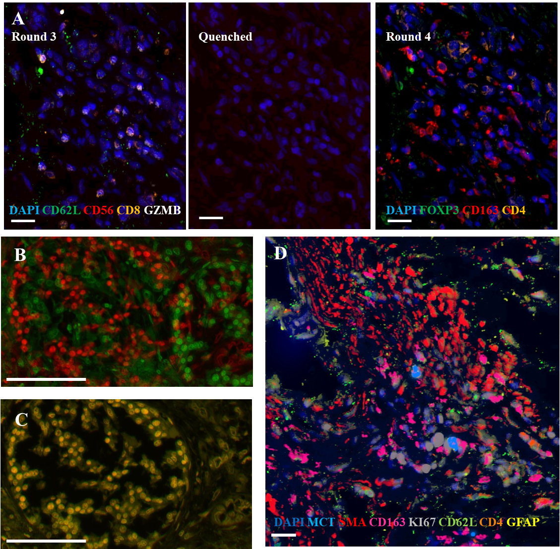
Figure 1.

Representative images from cyclic multiplexed-immunofluorescence (MxIF) labeling of a primary PDAC tumor with image registration. A) Images showing distinct marker distributions in the same area across staining round 3, quenching and re-scanning at the same intensity, and re-staining round 4. Scale bar = 20 μm. B) Unaligned image of DAPI staining of the same area from round 1 (green) and 9 (red) . C) Alignment (overlaid yellow) of round 1 and 9 DAPI using image registration software. Scale bar = 100 μm. D) Aligned composite image showing a subset of markers from different rounds of the MxIF panel. Scale bar = 20 μm.

2.3Multiplexed WSI image alignment and pre-processing

WSI images were converted from the proprietary 3DHistech file format (.MXRS), to an 8-bit universal file format (.TIF) for image registration and post processing. Additional information regarding the images and analysis regions are provided in Supplementary Table 1.

Using the above MxIF technique over 30 distinct markers and nine DAPI stainings were aligned. In each of the nine rounds of imaging additional channels align automatically to the corresponding DAPI channel; registration is required to align DAPI frames across rounds. Once DAPI frames are co-registered (see below, Fig. 1B–D), the same translation vector was applied to the associated marker frames bringing all 40 frames into alignment. The code for the registration software is available at GitHub (https://github.com/EDRN/slide-image-registration/releases/tag/v1.0.0).

For alignment of DAPI frames, the first DAPI frame was used as the anchor for subsequent the DAPI frames from all other rounds are registered. The registration method is based on cross-correlation in the frequency domain [18]. The scikit-image implementation of this method uses discrete Fourier transform to achieve arbitrary sub-pixel precision [19]. Frames with either dimension exceeding 30,000 pixels were down-sampled to accommodate larger frames in available memory, making it possible to apply the registration method to entire frames. When conducting cyclic MxIF and iterative WSI, artifacts due to varying staining intensities, tissue damage, or large over-exposed regions can introduce errors in registration [20, 21]. It is therefore important to visually or experimentally verify alignment fidelity. Outputs of the automated alignments were visually inspected and adjusted as needed (see below).

To remain within registration pipeline file size restriction, single channel images were limited to 1.5 GB and some images were cropped to maintain an appropriate file size. A 1.5 GB image still includes tens-of-thousands of cells for analysis. Once registered, successful global alignment was verified visually across all nine rounds of staining using DAPI staining (Fig. 1B and C). Minor misalignments that persisted were adjusted manually in GIMP (GNU Image Manipulation Program) which allowed manipulation of a set of images while preserving spatial consistency. Global alignment was verified visually in GIMP. Files exported from GIMP were converted to .PNG in ImageJ (National Institutes of Health) for background subtraction. We performed further verification of cellular alignment within HALO (High-Plex FL v2.0, see below). Similar analyses could be done visually though at a much larger time expense.

2.4Nuclear segmentation and antigen intensity quantification

Once aligned, nuclei were segmented based on each round of DAPI staining using HALO, a WSI software designed for cellular quantification. Within the HALO analysis platform, the nuclear segmentation algorithm was optimized based on a visual ground truth that could be applied to all images within our dataset. Nuclear contrast, segmentation aggressiveness, and intensity were set at 0.49, 0.795, and 0.05, respectively, using a one-point scale. Abnormally small or large cells were excluded. Segmented nuclei not present in each round of DAPI staining (non-high fidelity) were excluded from further analyses. High-fidelity cells were identified by consistent DAPI co-localization in the same location across all nine rounds of staining. This process excludes cells that go into or out of focus as the z-depth collection from the tissue can fluctuate slightly between scans or in areas lost to tissue damage over the de-coverslipping and re-staining process.

Using HALO, the average staining intensity was measured in the cytoplasmic and nuclear areas of high-fidelity cells. Staining intensity is based on the average number and intensity of pixels within the pre-defined area. The cytoplasmic area, the maximum range around the nucleus classified as the cell area, was set to 1.4 μm. When the cytoplasmic region intersects in multiple cells, HALO distributes available space evenly between the cells. For optimized training of the RFA, variables were decreased by averaging the intensity of each cell’s nuclear and cytoplasmic areas to produce one averaged numerical intensity output for each cell. Outputs were then Z-normalized to account for batch effect [22].

2.5Random forest classifier analysis of marker combinations

We applied a random forest classifier to investigate marker combinations classifying cells in stroma- and tumor-rich areas. Tumor and stroma regions were identified visually as MUC1 high or MUC1 low, respectively, with verification by a surgical pathologist. Normal adjacent or mixed tissue was excluded from analysis. Within our first pass analysis we considered all markers as potential predictors: [‘CCR3’, ‘CD103’, ‘CD11B’, ‘CD141’, ‘CD163’, ‘CD19’, ‘CD3’, ‘CD31’, ‘CD4’, ‘CD45RA’, ‘CD56’, ‘CD62L’, ‘CD8’, ‘CXCR3’, ‘EPCAM’, ‘FAP’, ‘FOXP3’, ‘GFAP’, ‘GZMB’, ‘IL10’, ‘INOS’, ‘KI67’, ‘LOX1’, ‘TRYPTASE’, ‘MPO’, ‘MUC1’, ‘PD1’, ‘PDL1’, ‘PRG2’, ‘SMA’, ‘VIMEN-TIN’]. Upon further analysis we removed markers suspected to be directly expressed on cancer cells (MUC1, Ki67, EPCAM).

We use scikit-learn implementation to train random forest models [19]. The training of random forest models is supervised, where all marker expression levels are matched with either tumor or stroma class in all data. In each image, there are different numbers of cells detected with the tumor and stroma regions (Supplementary Table 1). To address the effects of imbalanced tumor and stroma cell numbers in predictions, we used the balanced sampling strategy where class weights are adjusted to class frequencies for each tree being trained.

The number of trees and maximum tree depth were determined by monitoring the reduction of out-of-bag error with the addition of each new tree [23]. With all markers as predictors, we found the number of trees to stabilize around 150 trees with max depth of 30, beyond which adding new trees did not reduce the out-of-bag error significantly (Supplementary Fig. 1). While the out-of-bag error is an indicator of the model performance on the test set, cross-validation ensures all samples appear in the training and testing of random forests. We used 5-fold cross-validation with each set repeated ten times to report the average model performance in prediction accuracy.

To measure the importance of specific markers in predicting tumor vs. stromal regions, we used the feature importance scoring of random forest. The internal estimates at each tree node split (fig-single tree snippet) were used in measuring the predictor importance. The code for the RFA can be found at GitHub (https://github.com/EDRN/random-decision-forests/releases/tag/v1.0.0).

2.6Cellular clustering

Once the RFA was trained, top markers were used to identify cell groups based on Louvain clustering, an unsupervised algorithm designed to identify communities with similar features. Louvain clustering removes unintentional visual bias from the clustering method and has been used similarly on other large biological datasets [24, 25]. The Louvain clustering was run on all samples as one concatenated group. The outputs of Louvain clustering were verified with t-SNE plotting, a graphical output that compress high dimensional data onto a 2D plane in which like cells cluster with like. Cell types were then determined from this using heatmaps of the average intensity of all the antigens in each cluster and featured plots of the antigen distribution. Sub-gating (repeated Louvain clustering) was performed on a subset of clusters using the same technique

2.7Neighborhood construction and analysis

Following preprocessing of column structure and centroid calculation from bounding boxes, segmented cell centroids and Louvain-clustering classification were imported into Volumetric Tissue Exploration and Analysis (VTEA) and cellwise neighborhoods were segmented from a nearest-neighbor graph based on distances between cell centroids within 30 microns [26, 27]. VTEA was used to calculate the sum and fraction of the Louvain-cluster defined cell-types in each neighborhood and to export for further analysis in the R environment. Neighborhoods were analyzed in R using a modified neighborhood analysis workflow developed previously [28]. Neighborhoods were first preprocessed to exclude monotypic neighborhoods (one cell type) and then combined across patient samples. Using the total number of cell-types in individual neighborhoods, both Louvain-clustering and projections into t-SNE space were performed using the R packages knn and Rtsne. Stacked bar plots of the cell types in neighborhoods were assembled from total cells of a cell type per the total cells in a given neighborhood class. Code for VTEA is at: https://github.com/icbm-iupui/volumetric-tissue-exploration-analysis.

2.8Statistical analyses

Statistical analyses were performed in R and Excel, with p values of < 0.05 considered significant (*). An ANOVA was run on all multigroup datasets to verify significance. Student’s t-tests were used when comparing the mean expression values of individual markers. Data is presented in figures as the mean with standard error of the mean in brackets.

2.9Software and datasets

We have made the registered image sets from these analyses as well as the outputs from HALO following the Z-normalization publicly available at LABCAS (https://doi.org/10.26252/s18j-1h24). Our registration software and RFA are available on GitHub (https:// github.com/EDRN/slide-image-registration/releases/tag /v1.0.0 and https://github.com/EDRN/random-decision-forests/releases/tag/v1.0.0). The neighborhood analysis software is available on GitHub (https://github.com/icbm-iupui/volumetric-tissue-exploration-analysis). R Code for figure generation and analysis is available upon request.

3.1Image alignment

Image alignment accounts for slight alterations in slide position and scanning areas that occur when WSI is used over iterative staining rounds. Without correction, image misalignments could confound spatial information and co-localization data for multiplexed datasets. Figure 1C–E shows a successfully aligned area in comparison to pre-alignment images from the first and second round of staining, as well as an example area of high marker intensity post alignment (only subset of markers shown). When comparing segmented areas in the first round to high-fidelity nuclei/cells present throughout the whole staining cycle, we observed an average reduction of 48%. Based on visual inspection this decrease does not appear to be caused by tissue damage or alterations to the Z-depth while scanning but due to over-segmentation in the first round which fails to pass the requirements of high-fidelity cells (nuclear co-localization). There were no significant differences in spurious segmentations between the tumor and stromal tissue (data not shown).

3.2Validation of random forest algorithm

We developed a RFA to identify markers which define the tumor and stroma regions of the TME. Briefly, once slides are processed via MxIF analysis, images are divided into tumor or stromal rich regions (normal tissue and mixed excluded) and the RFA is trained on the presence or absence of markers in the tumor and stromal regions on all high-fidelity cells (Fig. 2). 70% of the cells within the sample were used for training, the other 30% were used for validation. The algorithm was cross-validated with a random selection of the 70:30 split each time to determine accuracy. This was done ten times per run. We tested our algorithm to both exclude and include MUC1, Ki67 and EPCAM, expected to be expressed on tumor cells and therefore an unnecessary bias/factor when seeking novel tumor, stroma predictors.

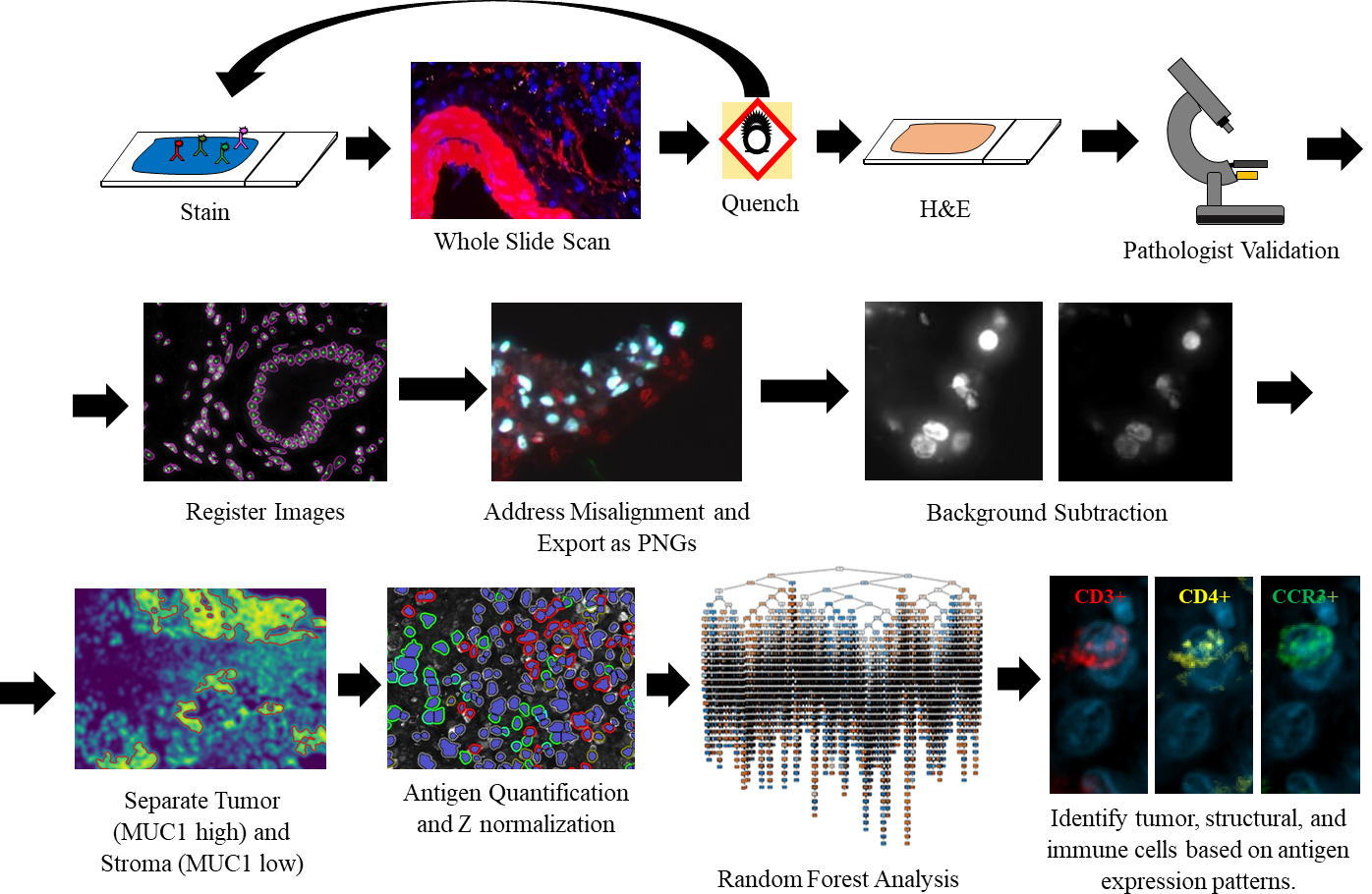
Figure 2.

Overview of the cyclic MxIF, WSI, and image analysis pipeline. After MxIF processing and pathological validation, images are aligned and classified for tumor-stromal content. Tumor and stromal areas were quantified separately and trained via the RFA. A limited branching decision tree is shown.

Among individual samples, we had very high accuracy of prediction (average 90.0% ± 0.001 (± SD) across ten runs per sample). Interestingly, excluding tumor markers (MUC1, Ki67, EPCAM) caused only a minimal decrease in the average accuracy (88.8% ± 0.002) indicating the algorithm can effectively predict tumor-rich areas of the TME without traditional cancer cell markers. When samples were concatenated and universally analyzed (excluding tumor markers) our predictive capacity dropped to slightly below the average of the individual algorithms (87.2% ± 0.001). We were also interested in the algorithm’s capacity to predict with a limited set of markers. We queried the algorithm to determine the top five markers driving tumor-stroma differentiation. As expected, we observed a decrease in the effectiveness of the algorithm when going from 31 to five markers; however, we were still able to predict the tumor and stromal regions with an average accuracy of 77.2% ± 0.001 across all samples. As we expand our sample set, we anticipate further increases in accuracy.

Figure 3.

Random forest outputs showing contributions of prediction driving markers in all, and those unique to representative long- and short-term survivor PDACs. A) Top 15 tumor-stroma predictors in all PDACs, excluding known cancer markers. B) Top 15 tumor-stroma predictors for long-term survivor (RAP 116), excluding cancer markers. C) Top 15 tumor-stroma predictors in short-term survivor (RAP 80), excluding cancer markers. D) Average marker rankings following jackknife resampling for top 15 markers.

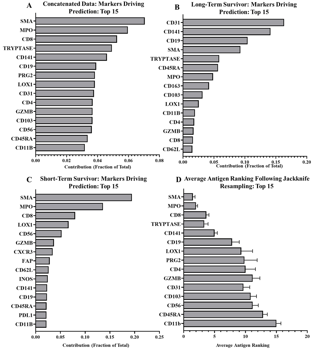
We additionally validated our algorithm by removing individual samples and repeating the RFA to determine if outlier expression was skewing the data set (jackknife resampling). While there were minor fluctuations, markers rarely shifted more than one to two positions in ranking following individual sample removal (Fig. 3D). This suggests the major drivers are particularly stable. Following this jackknife resampling we tested the RFAs produced against the sample that was removed and observed very minimal alterations to the efficacy of the RFA compared to the concatenated data (88.1% ± 0.012). All variable testing sets for the RFA, and their outputs can be found in Supplementary Table 3. The consistency of the RFA accuracy and marker rankings following jackknifing indicates consistent expression of specific cellular subsets within the tumor- and stroma-rich regions in the larger dataset.

3.3Random forest outputs

Using our RFA, we analyzed six primary pancreatic tumor samples to determine which markers were highly predictive of tumor and stromal regions of the TME. Among all our samples the strongest predictors were smooth muscle actin (SMA), myeloperoxidase (MPO), CD8, Mast Cell Tryptase, and CD141 (Fig. 3A). While we did see remarkable consistency within the marker ranking when jackknife resampling was applied to our patient cohort (Fig. 3D), there is variability between patients. Figure 3 shows the antigen rankings for a long-term and short-term survivor. In the long-term survivor (Fig. 3B), three antigens, CD31, CD141, and CD19 account for 50% of the drivers of prediction. The short-term survivor, matched for gender, age, and stage at diagnosis, presented with a different pattern of tumor-stroma drivers. SMA, MPO, and CD8 were among the highest predictors (Fig. 3C). Compared to the long-term survivor, CD19 (2.2%) and CD31 (1.9%) accounted for a very small prediction portion in the short-term survivor, suggesting patient-specific differences that may be related to disease aggressiveness. Looking at top drivers across patients though, clear consistent patterns emerge with Tryptase and SMA appearing among the top five drivers for five samples, MPO appearing in four, and CD8 and CD141 appearing in three. CD31 appeared twice among the top five drivers while CD56, LOX1, CD19, CD4, CD3, PDL1, CD103 and PRG2 appeared once (Supplementary Table 3).

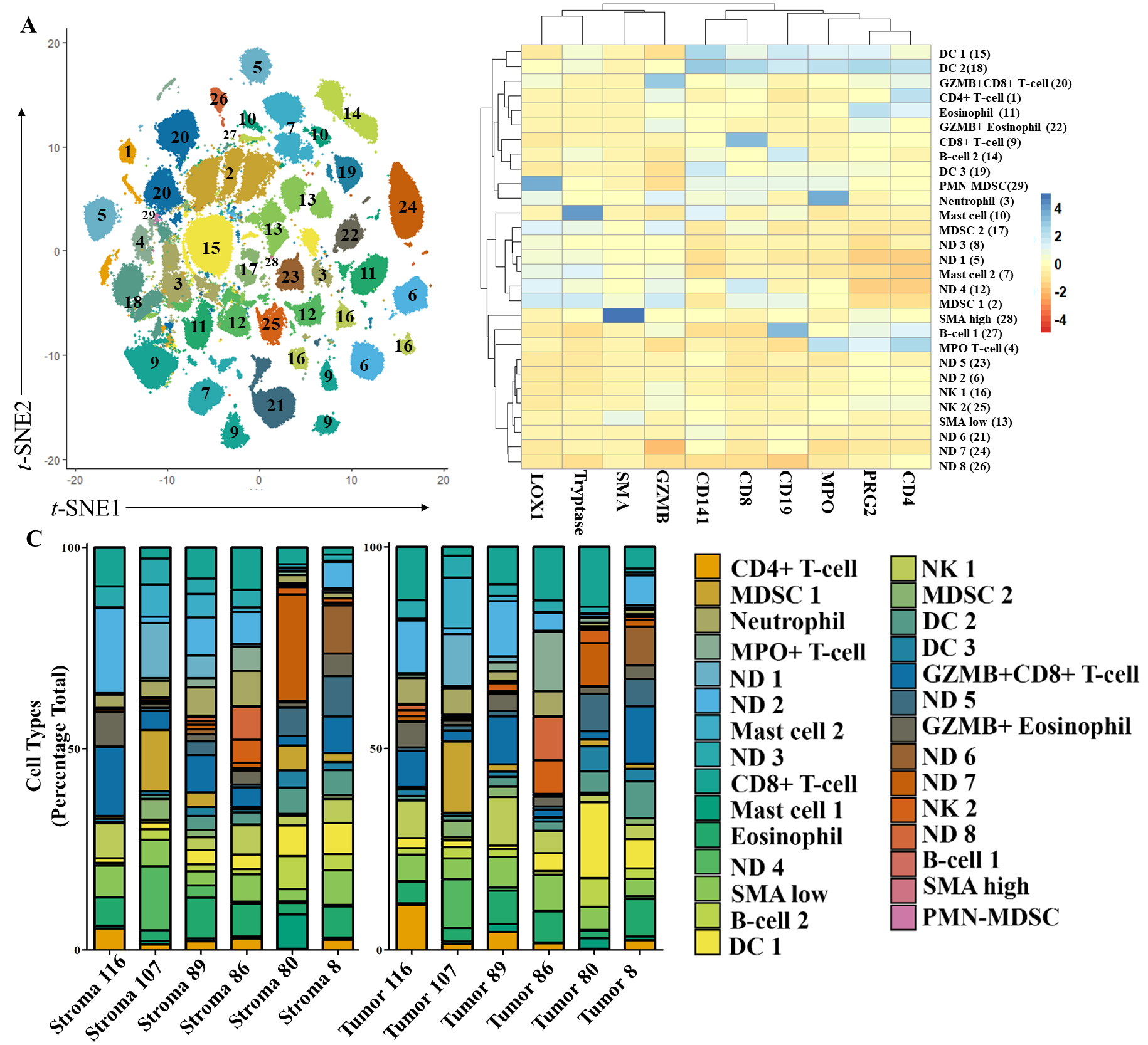
Figure 4.

Distribution of tumor-associated immune cells identified in PDAC TMEs using top ten tumor-predicting markers and unsupervised clustering. A) t-SNE plot of clustered cell groups (numbered) using RFA-identified antigens. B) Heatmap of the average cellular antigen intensity in groupings (see 4A) identified via Louvain clustering. Initial groupings shown in parentheses. C) Stacked bar plot of cell types identified with Louvain clustering of tumor and stroma tissues. Cell group colors matched in A and C.

3.4Identification of tumor- and stroma-specific cell types

To identify discrete cell populations present in tumor- and stroma-rich regions, we performed Louvain clustering using the top ten tumor-and stroma-driving antigens derived from the RFA. While CD31 was in the top ten driving antigens, we determined that more compelling cellular subtypes would be identified using GZMB which had a slightly lower score (0.0009 difference). Louvain clustering with GZMB grouped our dataset into 29 different clusters (Fig. 4A). Using antigen co-expression patterns on the heatmap (Fig. 4B) we were able to identify 21 different cell types in these clusters. Ten driver markers were sufficient for cell identification and allowed us to classify major immune cell subtypes in the TME. We observed expression patterns indicative of most major granulocytes, eosinophils (PRG2+), neutrophils (MPO+), and mast cells (Tryptase), as well as granulocytic-like MDSCs (MPO+, LOX1+, PMN-MDSCs). Of the adaptive immune response regulating cells, we identified clusters of B cells (CD19+) and CD4+ and CD8+ T cells. We also observed high and low levels of SMA expression. While SMA can indicate multiple structural components, high and low expression levels may additionally indicate inflammatory and myofibroblastic cancer associated fibroblasts, respectively [29].

By identifying 21 out 29 groups we were able to account for an average of 72% of cells within the TME. As our classification did not include cancer cells, this represents a sizable portion of cells in the TME. We did not observe significant differences in the number of identified cells between tumor and stroma regions, though a strong trend towards characterization of more cells within the tumor-rich regions was observed (data not shown). Notably, with the exception of the B cell cluster (group 27), all clusters were present all patients (Fig. 4C). While we observed strong trends in CD8+ T cell expression (group 9) increasing in the tumor-rich regions (p= 0.07), we did not see significant differences between the tumor and stromal regions. Based on our initial t-SNE plot (Fig. 4A) further sub-gating of the cells may be appropriate.

Figure 5.

Neighborhood analysis of all samples. A) t-SNE plot of spatial microenvironments (neighborhoods) and tissue distribution of neighborhoods between samples. Neighborhoods were classified by the distribution of cell types identified in Fig. 4. Red outline shows neighborhoods consistently recovered through all samples. B) Stacked bar plot of the cellular makeup of all neighborhoods. Approximate tissue distribution (bottom) from Supplemental Fig. 2, red indicates common neighborhoods. * indicates neighborhoods of future downstream focus. C) Correlation matrix of relationship between all cells in neighborhoods. Size and color indicate the Pearson’s correlation coefficient, positive (green), and negative (red) correlations are shown. Significant correlation (p< 0.05).

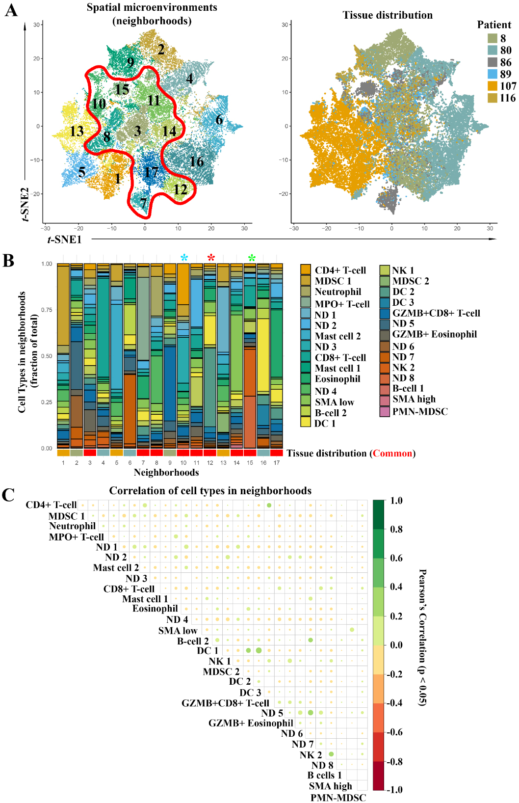
3.5Neighborhood analyses of cells in tumor- and stroma-rich regions

Based on the cell groups identified via Louvain clustering, we performed a neighborhood analysis on all cells within the tissue. We defined neighborhoods cell-wise as cells within 30 μm of each other and identified 17 unique types of neighborhoods following clustering (Fig. 5A). Our neighborhood analysis showed not all neighborhoods were present in each sample while some (9) are consistent across all patients (Fig. 5A). Several neighborhoods have clear, defining features. N7 is a granulocytic neighborhood with high levels of eosinophil and neutrophil markers while N17 is primarily composed of eosinophils. N10 represents the largest population of CD4+ T cell rich clusters while N15 is cytotoxic focused, with the largest grouping of NK cells and CD8+ T cells observed. N12 shows interestingly high levels of CD141 rich groups, indicative of DCs (Fig. 5B).

Next, we performed a correlation analysis for cell types within our neighborhoods and observed many significant correlations (Fig. 5C). Only significant correlations (p< 0.05) are listed. Among the CD4+ group we saw a strong correlation between CD4+ T Cells and CD8+ GZMB+ T cells and a weaker but still significant correlation to the CD8+ T cell group. Neutrophils had predominantly negative correlations to other identified cell types within the sample, including CD4+ and CD8+ T cells, mast cells, and DC subtypes. Both CD8+ T cell groups also had negative correlations spatially to eosinophils but positive correlations to B cells and other NK cell subtypes. Multiple DC populations correlated to our eosinophil group but not our GZMB+ eosinophil group which instead showed largely negative correlations. Interestingly, our DC cell populations predominantly show a negative spatial correlation to CD4+ and CD8+ T cells and a mixed relationship to B cells. DC 1 and DC 2 show a positive correlation to B Cell 1 but all DCs show a negative correlation to B cells 2. DC cells must physically interact with CD4+ and CD8+ T cells and B cells to present antigens for immune activation. Therefore, despite high DC populations in some patients, this is not necessarily sufficient to mount an active immune response as these cells are not spatially engaged.

Figure 6.

Sub-Gating of CD4+ and CD8+ T Cells, DCs, and NK cells. A) CD8+ T cell sub-gating using Louvain clustering (t-SNE plot) and GZMB distribution in CD8+ T cells (feature plot). B) Heatmaps of average marker expression in CD4+ T cells, CD8+ T cells, DC 2, and NK 2 cells. C) Stacked bar plot of CD4+ T cell, CD8+ T cell, DC 2, and NK 2 cell sub-gated cell groups in tumor and stroma regions in all patients. * =p< 0.05.

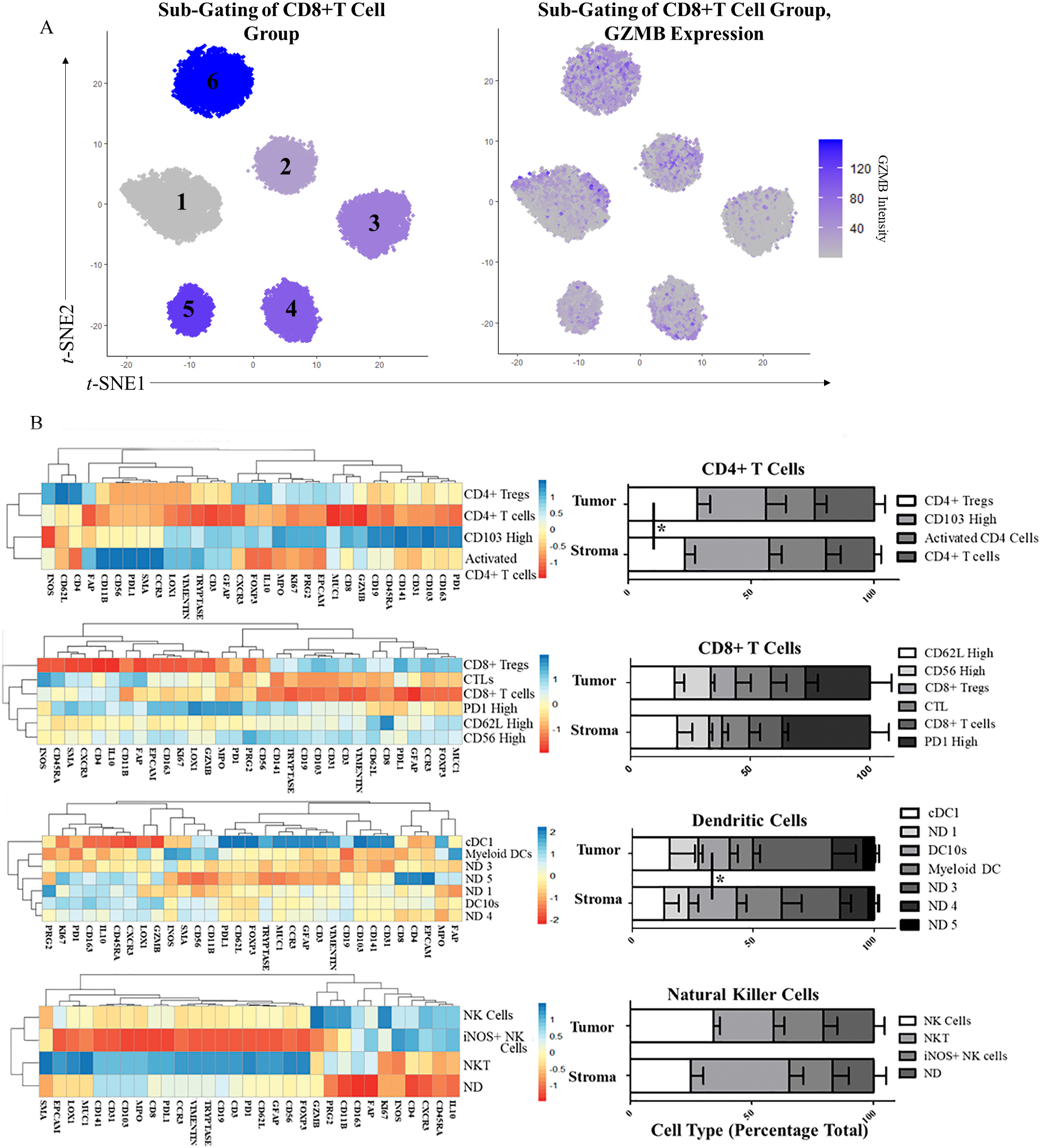
3.6Sub-classification of neighborhood-defining cell types

Following neighborhood classification of our samples, we identified cell types defining features of the neighborhoods that were consistent across all samples. We chose to further investigate CD4+ T cell populations, CD8+ T cell populations, and the DC 2 and NK 2 cell populations, as they made up the largest portion of the DC and cytotoxic neighborhoods, respectively. We repeated the Louvain clustering of these groups independently and were able to identify multiple cell types within each cluster (Example in Fig. 6A). Clustering with only the top ten antigens was sufficient for patterns to emerge from additional antigens uninvolved in the clustering and indicative of other unique cell types.

The CD4+ T cell Louvain clustering identified four groups (Fig. 6B). Using a heatmap of all antigens, we identified FOXP3 high CD4+ Tregs, GZMB high Cytotoxic CD4+ T cells, CD103 high CD4+ T cells, and CD4+ T cells which did not express activation or inactivation factors. We observed a significant increase in CD4+ Tregs in the tumor-rich regions (p< 0.05, Fig. 6B). By sub-gating the CD8+ cells we were able to identify six groups of cells; FOXP3 high CD8 Tregs, GZMB high CTLs; we also observed CD8+ cell clusters high in PD1, CD62L, and CD56 indicative of exhaustion or activation, memory or homing, and activation. CD8+ T cells that didn’t express any known activation or inactivation factors were additionally observed (Fig. 6B) [13, 14, 16]. Despite seeing a trend for increased CD8+ cells in the tumor rich regions, when subdivided, we did not see significant differences between the two groups (Fig. 6B). When sub-gating our DC 2 group, seven clusters emerged, three of which were identifiable cell types. CD141 high Cd11b high monocytic like DCs, CD141 high classical DC1s, (cDC1s) and CD163 and CD141 high cells, indicating DC10s [30, 31]. We observed a significant increase in the DC10 cell type in the stroma-rich region compared to tumor (p< 0.05). Among the NK 2 group, four clusters were defined with three unique cell types successfully identified: traditional NKs, NK T cells (NKT) high in CD56 and CD3, and NK cells high in iNOS. Within these groups there were trends towards increased traditional NKs in the tumor while NKTs were increased in the stroma (p= 0.062, p= 0.054, respectively).

3.7Cell type differences correlate with short- and long-term survival

Within our sample cohort we noted patient 116 was a uniquely long-term survivor at 497 days post diagnosis. All other untreated patients diagnosed at stage IV in our RAP cohort survived on average 96 days post diagnosis. We explored the cellular makeup of tumor and stromal regions from this long-term survivor (RAP 116) and compared those finding to a female patient of a similar age (RAP 80), also diagnosed in stage IV, who survived only seven days post diagnosis.

Figure 7.

Differential expression of tumor-associated immune cells in short-term (ST) and long-term (LT) PDAC survivors. Tumor- and stroma-specific cells samples sub-gated for DC 2 (A), CD4+ T cells (B), CD8+ T cells (C), and NK 2 cells (D).

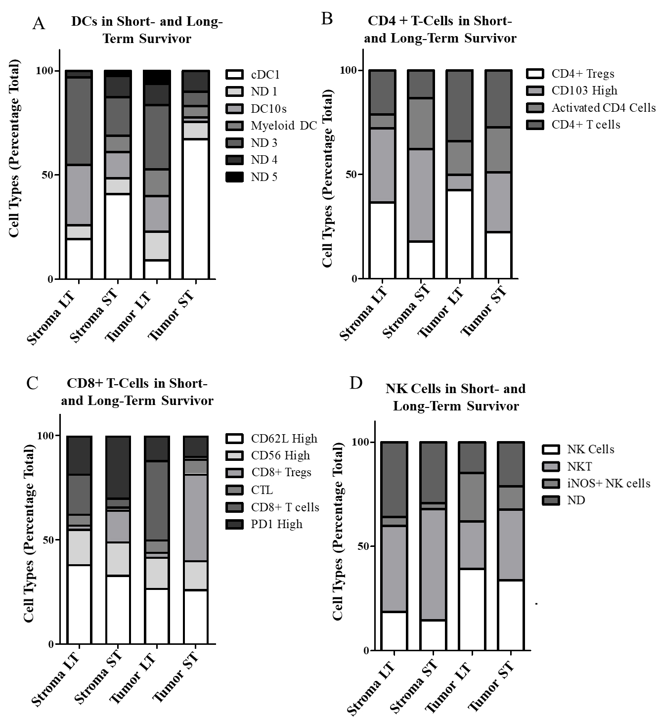
In the DC group, the long-term survivor had the lowest overall levels while patient 80 and 8, another particularly short-term survivor, had the highest levels (Fig. 4B). When sub-gated, most DC high cells in the short-term survivor were identified as cDC1s, while the long-term survivor had higher levels of myeloid like DCs and DC10s (Fig. 7A). The long-term survivor also had the highest levels of CD4+ cells of all patients. Surprisingly, the long-term survivor’s CD4+ cells were predominantly regulatory T cells. This is in contrast to the short-term survivor which had fewer regulatory T cells and higher levels of CD103 high T cells (Fig. 7B). Among CD8+ T cells, the short-term survivor had the highest level in the tumor-rich region but comparatively low levels in the stroma. When we looked at the tumor to stroma ratio of CD8+ expression, short-term survivors (RAP 8, 80), had the lowest ratio, while the long-term survivor was among the highest (Fig. 7C). Finally looking at our NK 2 cell sub-gating it is noteworthy that we saw the highest levels of NK cells within the tumor in the long-term survivor (Fig. 7D).

Looking at the overarching cell groups identified, we observed two B cell groups with an inverse relationships in long- and short-term survivors. In the B cell 1 group the long-term survivor had the largest population while they were conspicuously absent in the short-term survivor. In contrast, the short-term survivor (RAP 80) had the largest population of the B cell 2 group while the short-term survivor (RAP 116) had the smallest (Fig. 4B). Noteworthy from the correlation matrix (Fig. 4C) of the neighborhoods is that the B cell 2 group had a mostly positive correlation with DC cell clusters while the B cell 1 groups had a negative correlation. The CD8+ GZMB+ high clusters also made up a very large portion of the long-term survivor’s TME cells (Fig. 4B). There were no noteworthy features of granulocytic expression in the long-term survivor, though the short-term survivor had the highest level of mast cells of all patients. SMA expression was comparable across all patients.

To better characterize the spatial relationship of the cells we plotted the neighborhoods for all samples (Supplementary Fig. 2). We observed that the largest neighborhoods present in the long-term survivor (RAP 116) were N12, N8, and N7. In Fig. 5B, we can see these neighborhoods characterized as DC rich, granulocytic rich, and neutrophil rich, respectively. Interestingly, the short-term survivor (RAP 80) also has a very pronounced DC rich neighborhoods (N16 and N6) but this DC neighborhood is composed of different clusters of DC cells than those of the long-term survivor’s N12 neighborhood. It is also noteworthy that neighborhoods N16 and N6 have large populations of B cell 2 groups present. The short-term survival patient also had large CD8+ T cell rich neighborhoods (N4). This neighborhood is mostly populated by CD8+ T Cells, with very small populations of CD4+ T cells, NK cells, or B cells in the vicinity which could help orchestrate an adaptive immune response. Together this suggests less of a cytotoxic neighborhood and more of sequestered CD8+ T Cell neighborhood.

References

[1] | B.J. Kenner, S.T. Chari, A. Maitra et al., Early detection of pancreatic cancer-a defined future using lessons from other cancers: a white paper, Pancreas 45: ((2016) ), 1073–1079. |
[2] | Surveillance, Epidemiology, and End Results (SEER) Program Populations (1969–2018) [Internet]. National Cancer Institute, DCCPS, Surveillance Research Program. released December (2019) . |
[3] | X. Liu, J. Xu, B. Zhang et al., The reciprocal regulation between host tissue and immune cells in pancreatic ductal adenocarcinoma: new insights and therapeutic implications, Mol Cancer 18: ((2019) ), 184. |
[4] | M. Huber, C.U. Brehm, T.M. Gress et al., The immune microenvironment in pancreatic cancer, Int J Mol Sci 21: ((2020) ). |
[5] | A.N. Hosein, R.A. Brekken and A. Maitra, Pancreatic cancer stroma: an update on therapeutic targeting strategies, Nat Rev Gastroenterol Hepatol 17: ((2020) ), 487–505. |
[6] | S. Barua, P. Fang, A. Sharma et al., Spatial interaction of tumor cells and regulatory T cells correlates with survival in non-small cell lung cancer, Lung Cancer 117: ((2018) ), 73–79. |
[7] | Y. Masugi, T. Abe, A. Ueno et al., Characterization of spatial distribution of tumor-infiltrating CD8(+) T cells refines their prognostic utility for pancreatic cancer survival, Mod Pathol 32: ((2019) ), 1495–1507. |
[8] | J.L. Carstens, P. Correa de Sampaio, D. Yang et al., Spatial computation of intratumoral T cells correlates with survival of patients with pancreatic cancer, Nat Commun 8: ((2017) ), 15095. |
[9] | J. Watt and H.M. Kocher, The desmoplastic stroma of pancreatic cancer is a barrier to immune cell infiltration, Oncoimmunology 2: ((2013) ), e26788. |
[10] | J.R. Lin, B. Izar, S. Wang et al., Highly multiplexed immunofluorescence imaging of human tissues and tumors using t-CyCIF and conventional optical microscopes, Elife 7: ((2018) ). |
[11] | X. Wang, M. Lang, T. Zhao et al., Cancer-FOXP3 directly activated CCL5 to recruit FOXP3(+)Treg cells in pancreatic ductal adenocarcinoma, Oncogene 36: ((2017) ), 3048–3058. |
[12] | A.E. Prizment, R.A. Vierkant, T.C. Smyrk et al., Cytotoxic T Cells and Granzyme B Associated with Improved Colorectal Cancer Survival in a Prospective Cohort of Older Women, Cancer Epidemiol Biomarkers Prev 26: ((2017) ), 622–631. |
[13] | H.H. Van Acker, A. Capsomidis, E.L. Smits and V.F. Van Tendeloo, CD56 in the Immune System: More Than a Marker for Cytotoxicity? Front Immunol 8: ((2017) ), 892. |
[14] | E.I. Buchbinder and A. Desai, CTLA-4 and PD-1 Pathways: Similarities, Differences, and Implications of Their Inhibition, Am J Clin Oncol 39: ((2016) ), 98–106. |
[15] | J. Hang, J. Huang, S. Zhou et al., The clinical implication of CD45RA(+) naive T cells and CD45RO(+) memory T cells in advanced pancreatic cancer: a proxy for tumor biology and outcome prediction, Cancer Med 8: ((2019) ), 1326–1335. |
[16] | D.L. Woodland and J.E. Kohlmeier, Migration, maintenance and recall of memory T cells in peripheral tissues, Nat Rev Immunol 9: ((2009) ), 153–161. |
[17] | M.J. Gerdes, C.J. Sevinsky, A. Sood et al., Highly multiplexed single-cell analysis of formalin-fixed, paraffin-embedded cancer tissue, Proc Natl Acad Sci USA 110: ((2013) ), 11982–11987. |
[18] | L. Breiman, Random Forests, Machine Learning 45: (1) ((2001) ), 5–32. |
[19] | F.V.G. Pedregosa, A. Gramfort, V. Michel et al., Scikit-learn: Machine Learning in Python., J Mach Learn Res 12: ((2011) ), 2825–30. |
[20] | M. Guizar-Sicairos, S.T. Thurman and J.R. Fienup, Efficient subpixel image registration algorithms, Opt Lett 33: ((2008) ), 156–158. |
[21] | S. van der Walt, J.L. Schonberger, J. Nunez-Iglesias et al., scikit-image: image processing in Python, PeerJ 2: ((2014) ), e453. |
[22] | J.W. Hickey, Y. Tan, G.P. Nolan and Y. Goltsev, Strategies for accurate cell type identification in CODEX multiplexed imaging data, Front Immunol 12: ((2021) ), 727626. |
[23] | T.R.T. Hastie and J. Friedman, The Elements of Statistical Learning, 2 ed, Springer, New York, (2009) . |
[24] | H.W. Jackson, J.R. Fischer, V.R.T. Zanotelli et al., The single-cell pathology landscape of breast cancer, Nature 578: ((2020) ), 615–620. |
[25] | T.E. Bakken, N.L. Jorstad, Q. Hu et al., Comparative cellular analysis of motor cortex in human, marmoset and mouse, Nature 598: ((2021) ), 111–119. |
[26] | M.J. Ferkowicz, S. Winfree, A.R. Sabo et al., Large-scale, three-dimensional tissue cytometry of the human kidney: A complete and accessible pipeline, Lab Invest 101: (5) ((2021) ), 661–76. |
[27] | S. Winfree, S. Khan, R. Micanovic et al., Quantitative three-dimensional tissue cytometry to study kidney tissue and resident immune cells, J Am Soc Nephrol 28: ((2017) ), 2108–2118. |
[28] | B.B. Lake, R. Menon, S. Winfree et al., An atlas of healthy and injured cell states and niches in the human kidney, bioRxiv ((2021) ), 20212007.2028.454201.. |
[29] | C. Han, T. Liu and R. Yin, Biomarkers for cancer-associated fibroblasts, Biomark Res 8: ((2020) ), 64. |
[30] | M. Collin and V. Bigley, Human dendritic cell subsets: an update, Immunology 154: ((2018) ), 3–20. |
[31] | M. Comi, D. Avancini, F. Santoni de Sio et al., Coexpression of CD163 and CD141 identifies human circulating IL-10-producing dendritic cells (DC-10), Cell Mol Immunol 17: ((2020) ), 95–107. |
[32] | Z. Du, J.R. Lin, R. Rashid et al., Qualifying antibodies for image-based immune profiling and multiplexed tissue imaging, Nat Protoc 14: ((2019) ), 2900–2930. |
[33] | M. Comi, G. Amodio and S. Gregori, Interleukin-10-Producing DC-10 Is a Unique Tool to Promote Tolerance Via Antigen-Specific T Regulatory Type 1 Cells, Front Immunol 9: ((2018) ), 682. |
[34] | J.P. Bottcher and C. Reis e Sousa, The Role of Type 1 Conventional Dendritic Cells in Cancer Immunity, Trends Cancer 4: ((2018) ), 784–792. |
[35] | D.P. Xu, W.W. Shi, T.T. Zhang et al., Elevation of HLA-G-expressing DC-10 cells in patients with gastric cancer, Hum Immunol 77: ((2016) ), 800–804. |