
Probabilistic analysis of the effect of the combination of traffic and wind actions on a cable-stayed bridge
Abstract
At the design stage of bridges, all possible actions and their combinations are to be considered. In certain cases, the influence of the environment must be taken into account in addition to design values of traffic loads. In order to assess the current state of an existing bridge, actual applied actions must be considered: updated traffic situation, monitored climatic actions, and their unfavorable combinations. Therefore, monitoring all actions makes it possible to adequately study a structure. Since only limited data are generally available, the important question is how the quality and the duration of monitoring influence the assessment of the structure. In the current study applied to the Millau viaduct, effects from monitored traffic and wind actions are evaluated. The statistical analysis of applied actions and caused effects is done according to the Peaks Over Threshold (POT) approach. Results include the comparison between confidence intervals of predictions, for each studied load case and for various periods of monitoring. In addition, this paper presents study of the influence of the length of monitoring data on predictions of future extreme load cases, and also proposes an alternative efficient algorithm for threshold choice in the POT approach.
1Introduction
The complexity of predicting the residual life of large complex unique bridges such as the Millau viaduct is an important topic for the modern civil engineering work. Due to the fact that many European bridges, as well as bridges all over the world, are coming to the end of the design life, the question of the extension of their operational life is essential [1]. Moreover, some bridges were not designed to the current loading and have to be re-assessed. Studying such structures allows for improving the assessment of existing structures and possibly, gaining some profit from an economic point of view by avoiding unnecessary over-design or strengthening.
Usually, in bridge engineering and development of standards or norms, such as background works on the Eurocodes [2], the Extreme Value Theory (EVT) is used for forecasting of return levels of actions for the period of the interest. One of the most efficient approaches to be used is the Peaks Over Threshold (POT) method, that was not used during the mentioned background works, but which has proven to work well in diverse fields: wind engineering [4], precipitation predictions with non-stationary data [5], electricity demand estimation with a time-varying threshold [6], etc. Here, it is used for two types of loading – loading from heavy vehicles and wind loading, and their combination.
Concerning bridges, EVT has been successfully used to envision the forthcoming situation of structures [7, 8] based on the long-term monitoring of traffic actions. For the proper use of EVT, usually, only extreme actions (meaning the highest in absolute value) are considered. More precisely, heavy (even over-weighted) trucks are taken into account without paying attention to lighter vehicles.
Usually, bridges are designed against wind according to standards [9], considering the specific area of the location of the structure. As for effects of the wind on existing bridges, where applicable, much research have been made, and even more research are needed. For instance, the study of the aeroelastic behavior of long-span suspension bridges [10] shows the importance of wind effects, which can endanger the life of a bridge. Combining wind actions with vehicles as mass points [11] shows that higher wind speed actions do not necessarily cause a shorter life. However, the combination with trucks induces large stresses in the structure. In the current work, only static wind loads [12] are studied that simplifies the calculation process but makes it possible to observe conclusions based on available weather data. The considered direction of the wind (perpendicular to the deck) has been chosen after analyzing wind roses for the area.
The present work is devoted to the Millau viaduct, France, with the main aim in finding probabilities and effects of the combination of high velocity winds with heavy traffic for the most unfavorable cases. In order to use available monitoring data and to avoid additional assumptions, only static loads are considered without accounting for accelerations of traffic or dynamic wind effects. Based on techniques developed in the field of finance [13] and risk management [14], an updated algorithm is proposed for the threshold choice in the POT approach applied to traffic and wind actions that gives the best level of confidence for results. As well, the observation of the influence of a monitoring duration on load effects predictions is made to evaluate the validity of predicting critical load cases using limited monitoring information.
In this current paper, the following monitoring systems have been used: Bridge Weigh In Motion (BWIM), the principle of which was firstly proposed by Fred Moses [15, 16], installed underneath the deck slab, and the weather station information for the wind velocity. Following cases (and their combinations) are presented here:
• Traffic actions based on two months of BWIM data,
• Traffic actions based on six months of BWIM data,
• Wind actions based on the same period of monitoring as traffic,
• Wind actions based on historical data for the period of existence of the bridge.
2Millau viaduct
2.1Overview
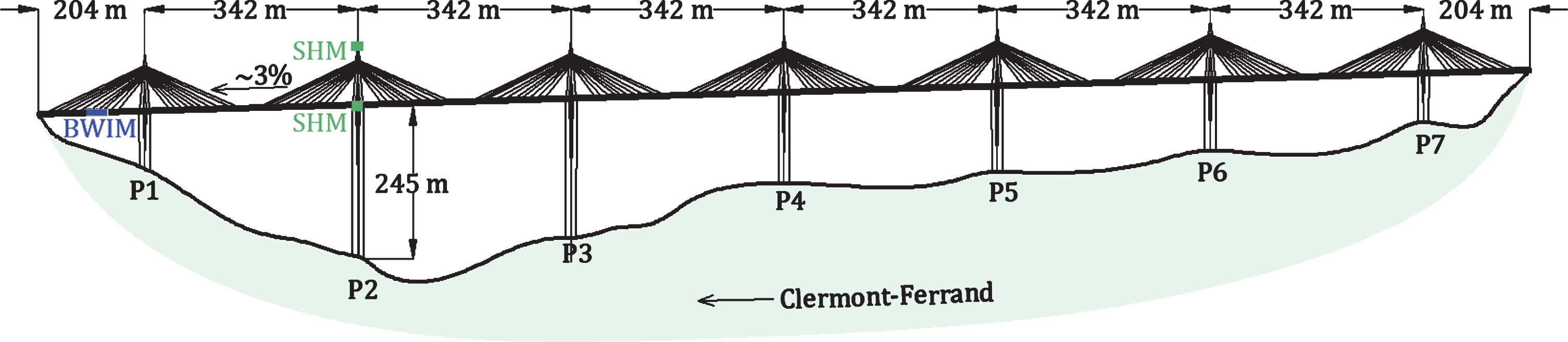
The Millau viaduct is crossing the valley of the Tarn river in Southern France. It is one of the highest cable-stayed bridges in the world, with piles of heights between 77 and 245 m, and pylons of almost 90 m of height (Fig. 1). Its steel orthotropic deck is composed of 342 m long spans with the total length 2460 m. Each span is suspended by 11 cables and provided with extension joints at the abutments [17], which permit openings up to 80 cm in the longitudinal direction. It is necessary to mention that span lengths (over 200 m) require specific studies, as their lengths are beyond those covered by the load models of the Eurocodes [18].
Fig.1
Scheme of the Millau Viaduct.
At the design stage of the viaduct, extreme wind actions were considered with a respect to site characteristics and the aerodynamic behavior of bridge elements. The possible effects are taken into account by safety factors obtained by both static and dynamic calculations [19]. One of the design deformed shapes: tower-lateral with some torsion in the deck (Fig. 2) brings attention to the combination of traffic and wind loads. Therefore, the case of congestion of heavy trucks and the static wind coming from unfavorable direction is studied further in the paper.
Fig.2
Schematic view of one of the deformation modes of the deck for the considered part of the bridge, [19].
![Schematic view of one of the deformation modes of the deck for the considered part of the bridge, [19].](https://content.iospress.com:443/media/brs/2019/15-3/brs-15-3-brs190151/brs-15-brs190151-g002.jpg)
2.2Objectives
The main aspect covered in this study is the prediction of extreme load effects based on monitored actions caused by the wind and traffic, both separately and combined together. These two loads are assumed to be statistically independent due to the absence of any recorded data on their dependency.
It should be noted that due to the safety regulations on traffic, the Millau viaduct is closed if the wind speed crosses 39 m/s (140 km/h), and lorry caravans are prohibited for wind velocities over 30.5 m/s (110 km/h). Therefore, the combination of traffic and wind is studied up to these values.
One of the objectives of this paper is the comparison between the probabilities of occurrence of extreme load effects for given return periods, based on various monitoring periods.
Let L1 and L2 be the statistically independent random variables of load effects, caused by two types of independent actions, which occur simultaneously. For k = 1, 2, ... let
(1)
In this work, random variables L1 and L2 are chosen to be the bending moment (BM) of the pylon P2 at the level of the deck caused by wind and traffic actions, respectively. The load effect L2 is given by a single heavy lorry or a group of several vehicles in order to find the most critical and the most probable cases.
Different traffic scenarios can be simulated to use measured traffic data and take into account various traffic situations, as it was done before by Monte-Carlo simulations [20] and traffic microsimulation [21]. Nevertheless, only lines of lorries are considered here as the comparison made in the current study covers static loading for both traffic and wind actions.
The static wind was chosen for the probabilistic model in order to observe the possibility of making such analysis if only simple data from a weather station is available: hourly wind speeds and directions. Therefore, results should not affect the Millau viaduct but allow to use it as a case study. The idea is to show, even if the information on the wind is not precise or not complete, that the probability for the combination of extreme cases of traffic and static wind actions is low compared to probabilities of extreme cases for each load separately.
2.3Monitoring of traffic
The deck of the Millau viaduct was equipped with a BWIM system for two short periods during years 2016 and 2017, in the same way as it has been done before [22]. Recorded data include information about every truck passing the bridge: type of vehicle, weights of each axle, distances between them, and speed.
The system itself was located in the middle of the first span (Fig. 1), inside the orthotropic deck, underneath the deck plate. The deck of the viaduct has two lanes in each direction, a slow and a high-speed lane. Monitoring has been done in the most loaded direction, which permits using recorded data for the mathematical model and theoretical predictions of traffic actions.
Figure 4 shows gross vehicle weight (GVW) of all recorded heavy trucks on both lanes. There are several interruptions in recordings, therefore, two sets of data are used here:
• October - December 2016 (43 days), called BWIM-I hereafter,
• February - July 2017, called BWIM-II hereafter (26, 67 and 40 days are considered as one measured period, and short pauses in monitoring during the year 2017 are not taken into account, assuming that the traffic was continuously being observed).
Fig.3
Cross section of the deck and traffic lanes.
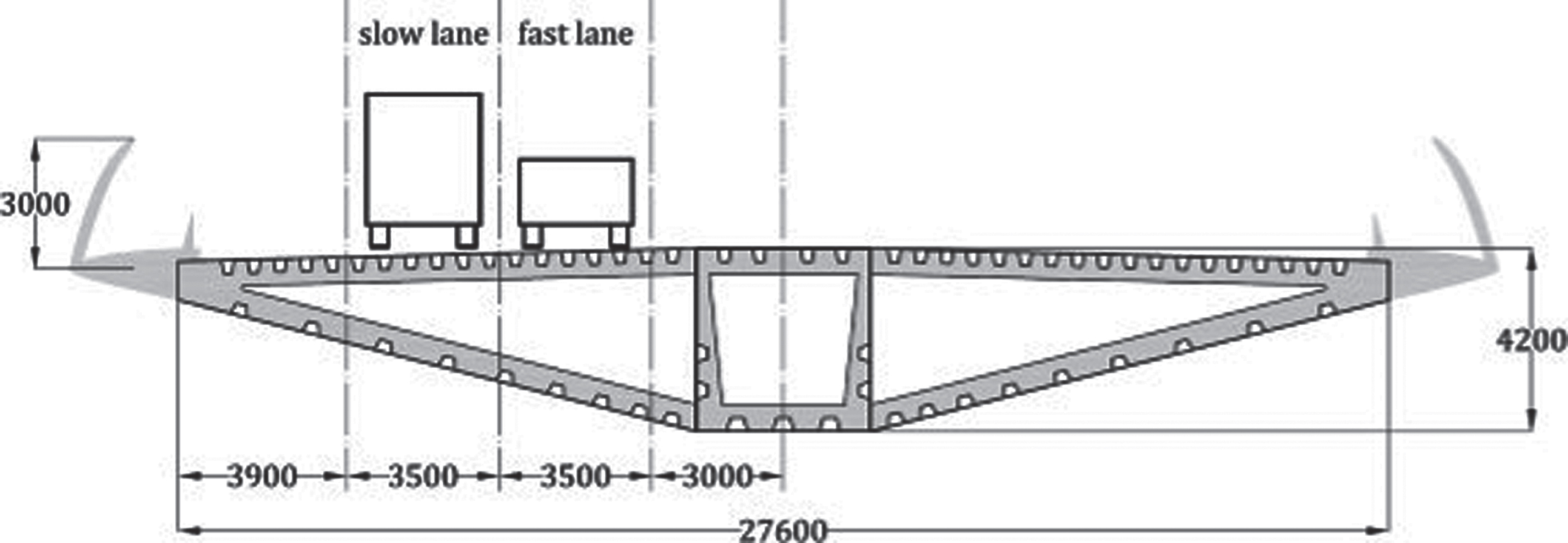
Fig.4
GVW of all vehicles recorded by BWIM system.
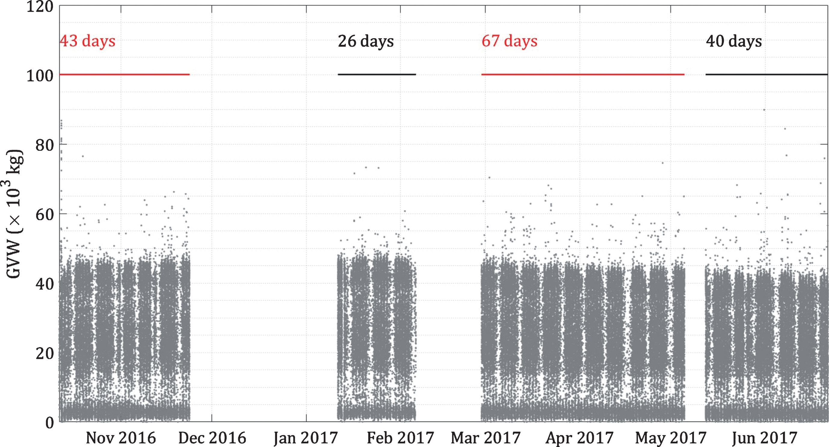
The advantage of the BWIM system is that it counts weights and records all vehicle passing over the instrumented section. The statistical distribution depends on many factors such as location, country regulations, time of the day, day of the week, and economical aspects. Changes in the economical situation cause increases or drops in traffic volume and brings doubts into the assumption of stationarity of traffic over time [23]. Nevertheless, the traffic growth is neglected here due to the fact that longer monitored data are not available. Moreover, weekly stationarity of traffic is assumed based on testing of time series for recorded traffic. It can be clearly observed from Fig. 4 that the distribution of vehicles weights and numbers repeat itself every week with slight seasonal change.
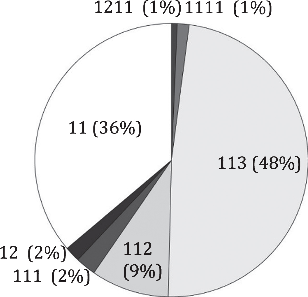
For the considered period, the most common type of vehicles is a 5-axles truck ”113” (composed of two single axles and a group of three axles), which is common in France. The second popular type is a two-axles van ”11” (two single axles), followed by four-axles “112” (two single axles followed by a tandem) and a few more (“111”, ”12”, “1111”, “1211”). The proportion of each type is shown in the pie-chart of Fig. 5.
Fig.5
Most frequent axles combinations.
For the extreme value analysis using POT approach, only the highest values are considered. All data are presented in Table 1. The fourth column shows the limit for GVW in France for a given number of axles [24], and the sixth and eighth columns give the proportion of overloaded trucks.
Table 1
Monitored data for different types of trucks
| Axle type | Image | % | Allowed GVW, (×103 kg) | I – 43 days | II – 176 days | ||
| Total recorded | GVW over limit (%) | Total recorded | GVW over limit (%) | ||||
| “113” |  | 47 | 44 | 17611 | 12.1 | 76754 | 7.0 |
| “11” |  | 35 | 19 | 12781 | 1.1 | 57442 | 0.7 |
| “112” |  | 9 | 38 | 3489 | 1.2 | 14658 | 1.0 |
| “111” |  | 2 | 26 | 878 | 2.9 | 3827 | 3.0 |
| “12” |  | 2 | 26 | 589 | 11.4 | 2908 | 8.7 |
| “1111” |  | 1 | 32 | 518 | 7.9 | 2211 | 8.8 |
| “1211” |  | 1 | 44 | 264 | 3.4 | 1084 | 3.3 |
2.4Data collection for the wind
In order to observe the influence of some climatic conditions (here, the wind), the global effects on the entire structure are considered. The wind profile is formed according to the wind data at four different heights of the pile P2 with its pylon collected by the Bridge Management System (BMS) and a national weather station located nearby.
First of all, data from the Structural Health Monitoring (SHM) system installed in the structure is used. It includes measurements of wind speeds and directions at the level of the deck and at the top of the highest tower. The SHM system is operating only if the wind speed up-crosses the value of 25 m/s [25], which is not sufficient for the statistical analysis and for making predictions. For research purposes, during one week (16–20 May 2017) the SHM system was turned on during working hours to observe the values of the wind near the bridge structure (the example of recorded signal is shown in Fig. 6) and compare these values with those of the weather station. The following conclusions can be made based on provided results:
• The values of hourly mean or maximum of wind speeds are used in the further predictions: according to experience [26], these values are considered as independent observations of the wind speed.
• One of the most frequent directions is perpendicular to the longitudinal direction of the bridge deck (winds from North-West, Fig. 7), that brings attention to both limit states – ultimate (ULS) and serviceability (SLS), of the deck of the viaduct (Fig. 2) including possible torsion in the deck.
• The wind speed at the top of the tower is about 20% higher than at the level of the deck (Fig. 8), which makes it necessary to take this difference into account in calculations.
Fig.6
Recorded wind speeds at the top of P2 of the Millau viaduct.
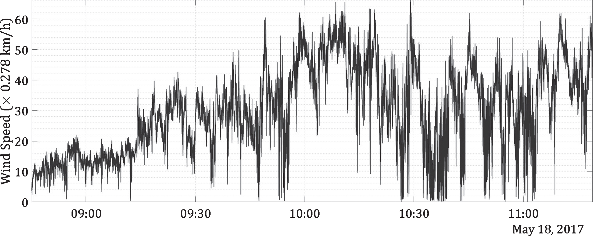
Fig.7
Wind roses for the top of the pylon P2 and for the weather station in Creissels.
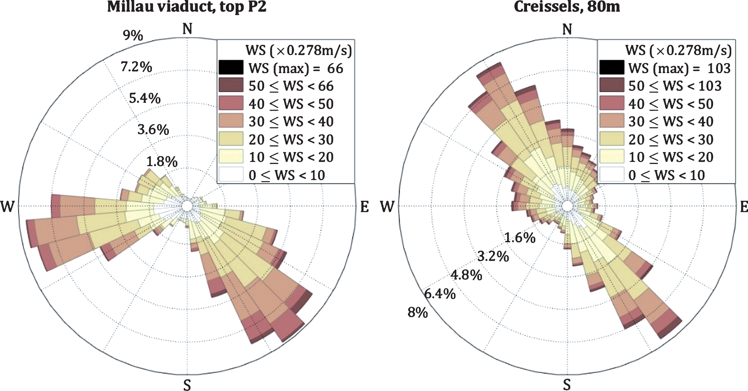
Fig.8
Wind speeds at different levels based on different recorded data for Millau viaduct.
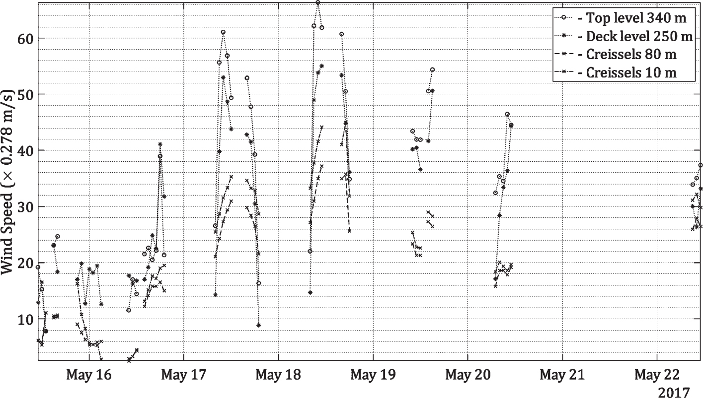
Secondly, weather data for wind velocities in the area are coming from the climatic station located nearby, in Creissels, and comprise values of wind speeds and directions for each hour at the height of 80 m above the ground. To obtain values of the wind speed at the level of the deck (249 m height) and at the top of P2 (339 m height) of the viaduct, a simplified calibration has been done depending on the mean values of differences between wind velocities at several heights. Monitored wind velocities for certain hours between 16th and 20th of May, 2017 (Fig. 8) are compared with wind velocities from the Creissels weather station.
Figure 8 shows that the ”peaks” of velocities arrive approximately at the same time. The random variables represent the differences of wind speeds between several heights (the Creissels weather station, the deck and the top of the pylon P2 of the Millau viaduct). From the measurements, the statistical estimation of their probability distribution functions show that these random variables are approximately Gaussian. Only velocities of more than 30 km/h are considered.
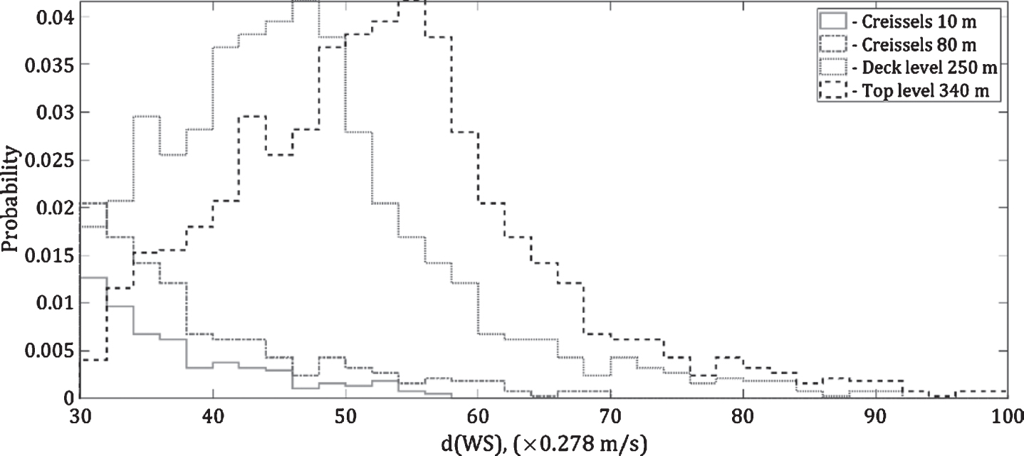
The period of weather data is chosen to be the same as for the monitoring of traffic: (11/10/2016 – 21/06/2017). The obtained histograms of wind speeds for the given period are shown in Fig. 9. In the considered direction, the maximum wind speed recorded during this period is 55 km/h. The 95% -estimate of the confidence interval of wind speed is 74.6±10.4 km/h at the top of the pylon and 68.6±8.4 km/h at the deck level. The values of the wind force as a function of the wind speed are summarized in Table 8 in Appendix D.
Fig.9
Histogram of the wind speeds at different levels for the period Oct 2016 June 2017.
In addition, due to the availability of data and for statistical calculations, these data were updated twice: one with the period of bridge operation (16/12/2004 – 01/03/2018) and one with the entire period of available climatic data at the Creissels weather station (01/01/1985 – 01/03/2018) in order to observe the influence of monitored duration on results.
3Prediction of load effects
3.1Methodology
3.1.1Calculation of load effects
Two available periods of traffic measurements allow for comparing predictions made by using short time (43 days) BWIM-I monitoring with results based on a longer period BWIM-II (176 days). The action of the wind is taken into account as a separate static load coming from the most unfavorable direction. Three periods are considered: WS-I – the same period as BWIM-II (2016-2017) and WS-II – the operating life of the bridge at the moment (2004-2018). In addition, the entire available statistical data for wind WS-III (1985-2008) is used to compare results obtained for various lengths of monitoring duration. Both types of actions have been combined, based on the period from October 2016 until June 2017.
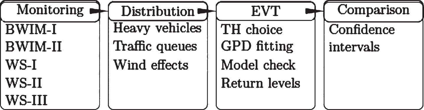
These measurements provide sets of values that form vectors of load effects (LEs), which are used in the EVT, based on the block and the threshold models [3], where only extreme effects are considered. Data are fitted to the generalized Pareto distribution (GPD). The confidence intervals (CIs) of return levels (RLs) are compared. Figure 10 represents the different steps of the procedure that are used for each case. The return levels are estimated for the guaranteed lifetime of the bridge of 120 years [27].
Fig.10
Extreme value assessment procedure.
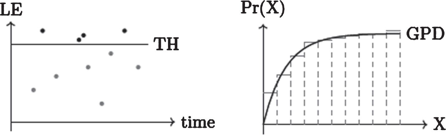
The methodology for the application of POT (Fig. 11) to recorded load effects and for the calculation of the return levels is given in Appendix A. The evaluation of confidence intervals is detailed in Appendix B. The main drawback of the approach is the choice of a threshold, therefore, an updated algorithm is provided based on previous works in other fields [13, 14].
Fig.11
Representation of the POT approach.
3.1.2Updated methodology for threshold choice
One of the most used ways to estimate the threshold is the mean residual life plot. The idea is to choose a sufficiently high limit so that values exceeding it are well fitted to the GPD with corresponding shape and scale parameters. To reach that, the threshold is usually taken at the tail of the Mean Residual Life plot (MRLP) when the function of the mean value excesses begins to be less curvy and has a tendency to be linear. Basically, the mean residual life plot (MRLP) is given by the set ζ of the “locus of points” (2) such that for an element xi of the load effect, which exceeds a threshold u, with i = 1, ... , Nɛ and Nɛ the total number of excesses,
(2)
Another solution used is checking several different thresholds by evaluating of confidence intervals for return levels.
Let U = U0, ... , Uk, ... , Up be the sequence of thresholds with U0 corresponding to the value of 90% -quantile (as it was concluded to be the most appropriate choice, for instance, in the recent study for temperatures [28]) and Up corresponding to the value of 99% -quantile (as higher values of threshold would lead to an insufficient number of excesses Ne,k to fit GPD). By substituting U into Equation (13) of Appendix A, we obtain a sequence of confidence intervals C(U) and for each Uk, the probability of exceedance is written as
(3)
in which Ntot is the total number of load effects.
Then, both C(U) and ζu(U) are plotted in the one graph in order to choose the threshold that gives the smallest value of the confident intervals.
In the current section, the methodology according to the EVT is described. However, the motivation for the choice of a threshold level comes also from the design and serviceability purposes. For instance, the choice of a threshold for traffic can be also explained by traffic regulations in France, where the value of the gross vehicle weight for 5-axles vehicles should not exceed 44 tons [23].
3.2Return levels for traffic
3.2.1Case of a critical single vehicle
It is necessary to take into account that 5-axles vehicles are often transporting goods in groups of two, three or four trucks. Analyzing time-series data available from the BWIM monitoring and recorded speeds of vehicles, situations with the presence of several heavy vehicles on one span at the same time were detected. This allows for assessing probabilities of occurrence (Table 2) of such situation that can lead to larger values of overall load effects. As 90.5% of time, a passage of a single vehicle takes place, the results are obtained, first of all, for this case.
Table 2
Occurrence of 5-axles trucks
| Number of 5-axles trucks in the queue | Total number of occurrences | Per week | Mean mass of one vehicle (×103 kg) | Total mass (×103 kg) | % of occurrences |
| 1 | 70412 | 2708 | 32.6 | 32.6 | 90.460% |
| 2 | 7024 | 270 | 33.0 | 66.0 | 9.024% |
| 3 | 389 | 15 | 32.7 | 98.1 | 0.500% |
| 4 | 11 | 0.5 | 29.2 | 116.8 | 0.014% |
| 5 | 2 | 0.08 | 29.9 | 149.5 | 0.002% |
The distribution of single vehicles is made for each group (Fig. 5), separately and for all vehicles together. Calculations are made using the algorithm explained in Section 1 (Fig. 12).
Fig.12
Steps to be taken in POT approach.

1. The first difficulty of the POT approach is finding a correct threshold. It is done here by different procedures:
a. observing the MRLP [3] according to Equation (2) in Section 3.1.2 and Appendix A, an example is given in Fig. 13 for axle type ‘1111’,
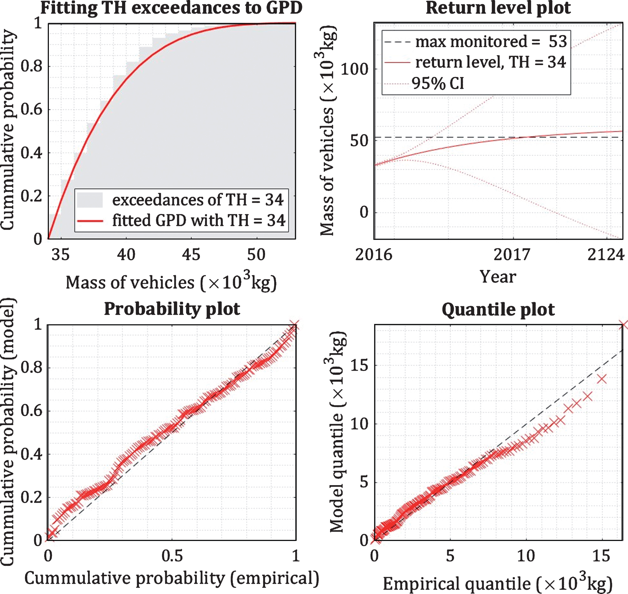
b. checking several different thresholds with corresponding model checking and evaluating the confidence intervals for return levels, as it is explained in Section 3.1.2. The algorithm has been programmed in MATLAB and the same example (axle type ‘1111’) is presented in Fig. 14. This figure shows two curves: confidence intervals and probability of exceedance as a function of a TH (threshold). The best value of a TH is where the confidence interval has a minimum value and the probability of exceedance stays inside an accepted range [90 ... 99%] yielding TH = 34.
2. At the next step, the GPD defined by Equation (11) in Appendix A, is estimated as to the distribution of “extreme” load effects – effects that lay over chosen TH – with the corresponding (fitted) parameters.
3. The analysis of the quality of the estimation is done by probability and quantile plots (e.g. Fig. 15). Empirical points (cross symbols in Fig. 15) are placed in order and they should tend to be linear following the theoretical curve (dashed line in Fig. 15). This is followed by ks-tests [29] based on differences between empirical and theoretical distributions.
4. Return levels are assessed according to Equation (12) in Appendix A for the return period equal to the design life of the bridge using estimated GPD shape and scale parameters.
5. The last step is the calculation of 95% confidence intervals for the computed return level (e.g. Fig. 15, dashed lines) according to Equations (13) to (17) in Appendix B.
Fig.13
Threshold choice (a) by MRLP for the mass of traffic.
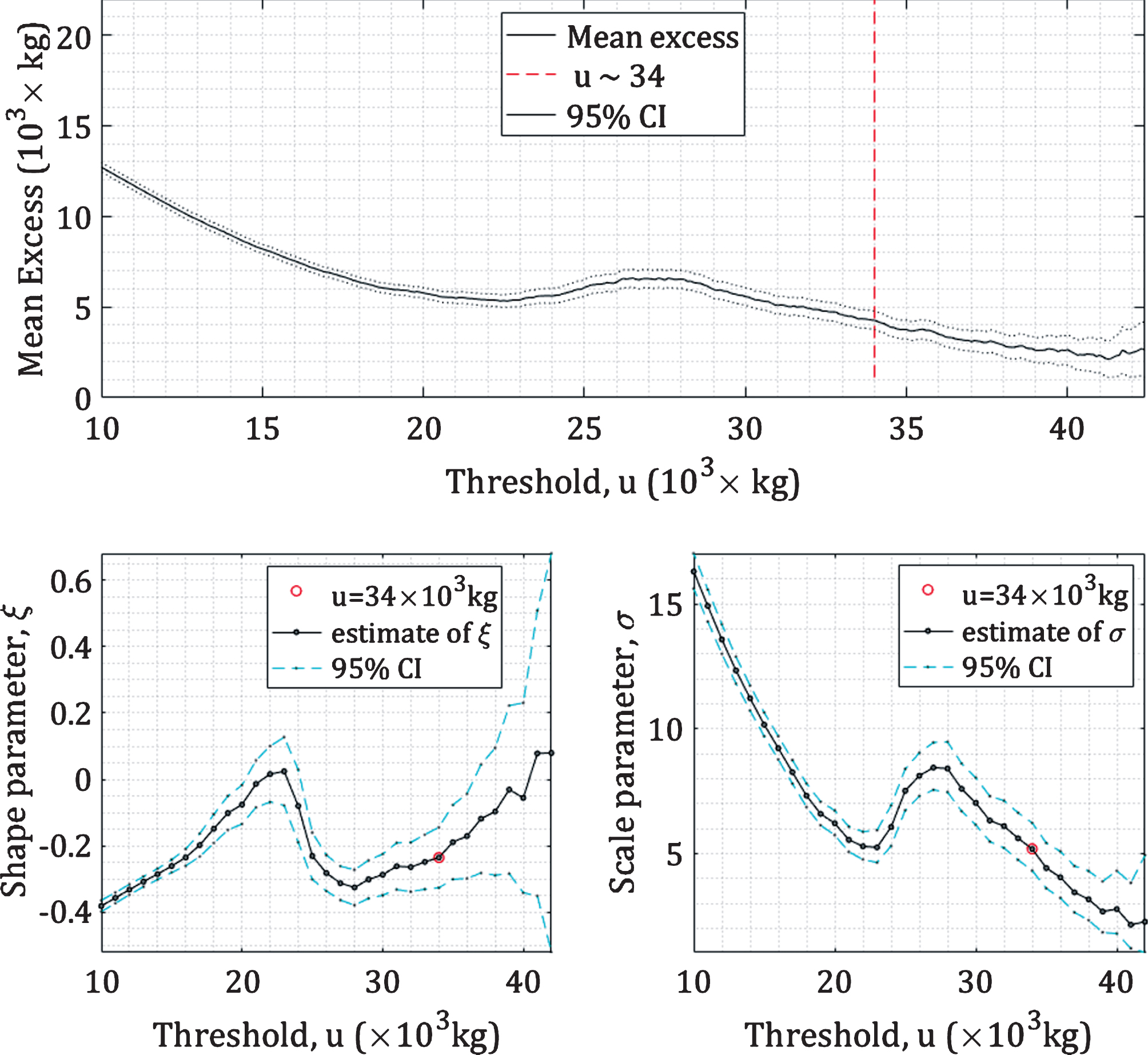
Fig.14
Threshold choice (b) depending on confidence intervals and the probability of exceedance.
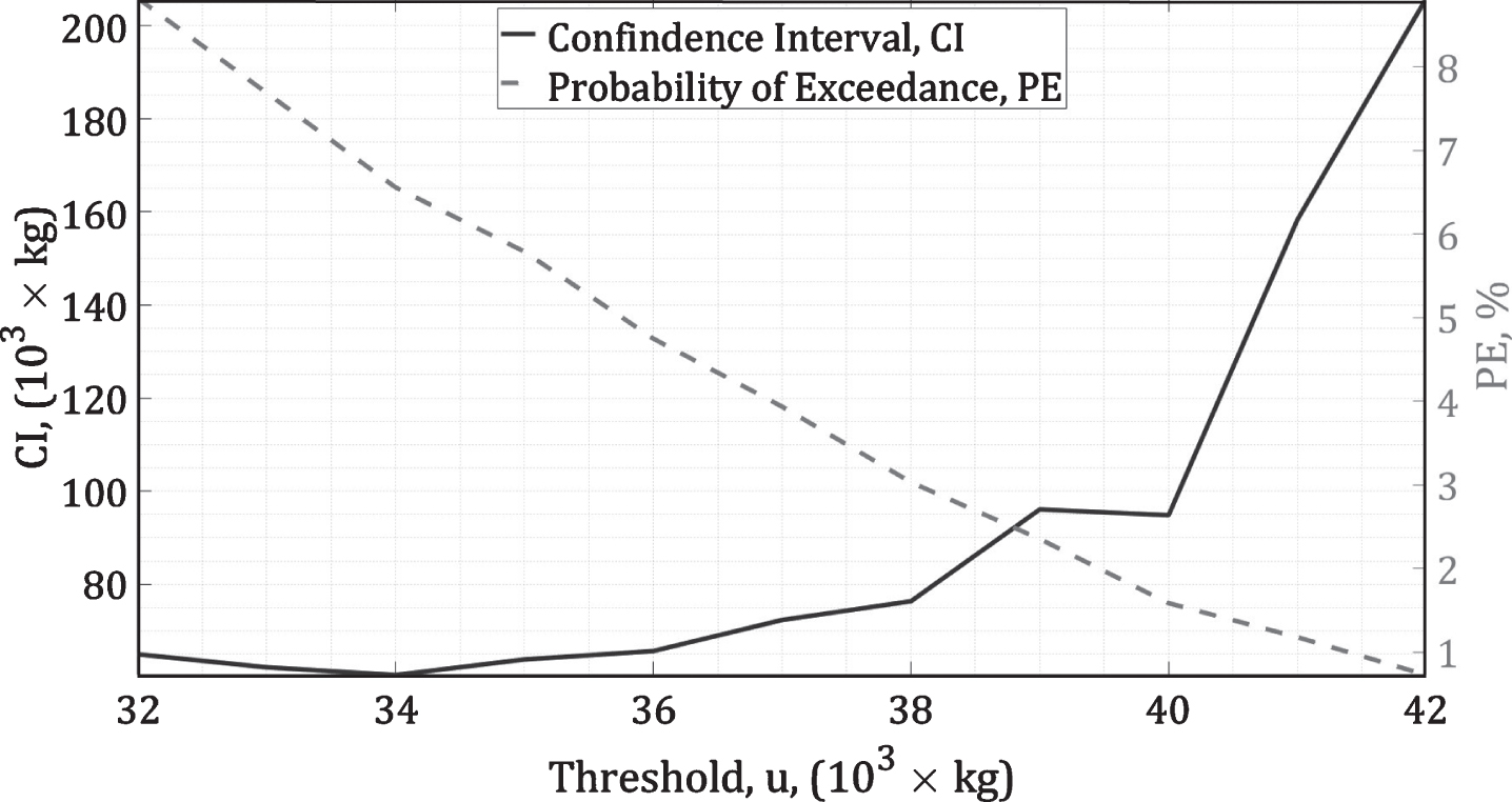
Fig.15
Analysis of the quality of the estimation.
For the first part of the study BWIM-I, only 43 days of data were available. The calculations were done according to the presented algorithm and the results are summarized in Table 3. For each type of vehicles, allowed weight and maximum recorded are provided, as well as the number of monitored trucks per day. Table 3 also includes TH chosen by proposed alternative method for each axle type and the percentage of vehicles weights over this TH. Moreover, the return levels and the confidence intervals are presented for the return period of 120 years - the guaranteed lifetime of Millau viaduct - as it was mentioned in Section 2.1. It is more difficult to fit the distribution when there are not much data available as, for example, “1211” with only 6 trucks per day. Therefore, the confidence intervals are too large to rely on values of the return levels. Comparing the column “113” with “ALL”, it is obvious that the heaviest and most frequent type of trucks is contributing the most into the entire picture, since the value of both the return levels and the confidence intervals is approximately the same for both cases.
Table 3
Return levels with confident intervals based on BWIM of 43
| Axle Type | “11” | “12” | “111” | “112” | “113” | “1111” | “1211” | ALL |
| Allowed GVW | 19 | 26 | 26 | 38 | 44 | 32 | 44 | 44 |
| Max recorded | 32.8 | 41.2 | 35.7 | 47.8 | 86.7 | 45.3 | 62.5 | 86.7 |
| Trucks | 297 | 14 | 20 | 81 | 410 | 12 | 6 | 841 |
| Threshold | 17 | 29 | 26 | 35 | 44 | 34 | 41 | 44 |
| Pr(X > TH) | 3% | 4% | 3% | 3% | 12% | 6% | 9% | 6% |
| RL, 120 years | 39 | 47 | 37 | 54 | 169 | 55 | 162 | 169 |
| CI | 36 | 222 | 56 | 59 | 78 | 65 | 1119 | 78 |
| RL + CI | 75 | 269 | 93 | 112 | 246 | 120 | 1281 | 248 |
The second part of the work, BWIM-II, includes all data available after the second installation, in total, 176 days. The same procedure is applied in order to obtain the return levels and the confidence intervals for GVW of all types of trucks. Results allow for updating the value of the confidence intervals. Table 4 shows that adding more data (longer period of measurements) permits to decrease the values of the return levels with the corresponding confidence intervals if the recorded maximum stays the same.
Table 4
Updated return level with confidence interval based on BWIM-II of 176 days with same thresholds
| Period | Maximum Recorded (×103 kg) | Trucks per day | TH (×103 kg) | Pr(X > TH) | RL (×103 kg) | CI (×103 kg) | RL+CI (×103 kg) |
| 43 days | 86.7 | 841 | 44 | 6% | 169 | 78 | 248 |
| 176 days | 86.7 | 903 | 44 | 3% | 113 | 28 | 141 |
3.2.2Case of a queue of lorries
All calculations are shown for a passage of a single truck. As for queues of lorries, for predictions of return levels, the mean value of the vehicle mass is used in each case according to Table 2. Table 2 gives numbers of occurrence of single 5-axles vehicles, groups of two, three, four and five 5-axles vehicles, as well as the mean and total mass for each case. The expected GVW in 120 years caused bending moment and the corresponding probability are computed. Bending moments caused in the structure are shown in Table 9 in D.
3.3Return levels for wind
The procedure explained in Section 3.2 (see Fig. 12), is also applied to the wind loading. Table 5 represents values of the return levels and the confidence intervals for the wind. The wind pressure is calculated with the wind speeds. As described in Section 2.3, wind speeds have been measured in two elevations: one at the level of the deck and one at the top of the pylon of the highest pile P2. In this work, the main objective is to analyze the influence of the combination of the wind load and the traffic load. The probability of occurrence of the wind NW direction, considering only four possible directions, is given in the second column of Table 5. Even if the measured values are not so high, it is possible to combine strong winds occurring in the perpendicular direction to the deck with heavy trucks passing in lane I (slow lane, Fig. 3) that is closer to the edge of the deck. Therefore, the next step is the combination of effects caused by both loads together.
Table 5
Results for return levels and confidence interval for the wind data collected at Creissels
| Based on data at 80 m height | Probability of occurrence of the wind NW direction, for 4 possible directions | Wind speed (×0.278 m/s) | Over TH (%) | |||
| Max | TH | RL | CI | |||
| 1985-2018, 12113 days | 0.378 | 119 | 55 | 134 | 219 | 1 |
| 2004-2018, 4824 days | 0.387 | 103 | 55 | 110 | 203 | 0.4 |
| 2016-2017, 254 days | 0.305 | 69 | 55 | 70 | 119 | 0.6 |
3.4Combination of the wind and traffic actions
3.4.1Bending moments
Prediction of traffic weights and wind velocities has been done in previous sections. In order to pass from actions to their effects, the bending moments (BM) at the level of the deck are found for both types of actions, as well as for their combination. Figure 2 displays a schematic view of the deformation (see Section 2.1) for the highest pile of the bridge. To obtain the response of the part of the bridge (see Fig. 16, left), a static linear 2D beam finite element model of the pile P2 with its pylon has been developed using MATLAB (see Fig. 16, middle). Traffic forces are directly obtained from known weights coming from BWIM data. The wind forces are calculated according to the general formula proposed in standards [9], see Annex C. Both monitored maximum actions and predicted actions at the end of the lifetime are applied to this part of the structure.
Fig.16
Part of the bridge considered for the 2D computational model (left), scheme of the pile with its pylon P2 (middle), 2D computational model (right).
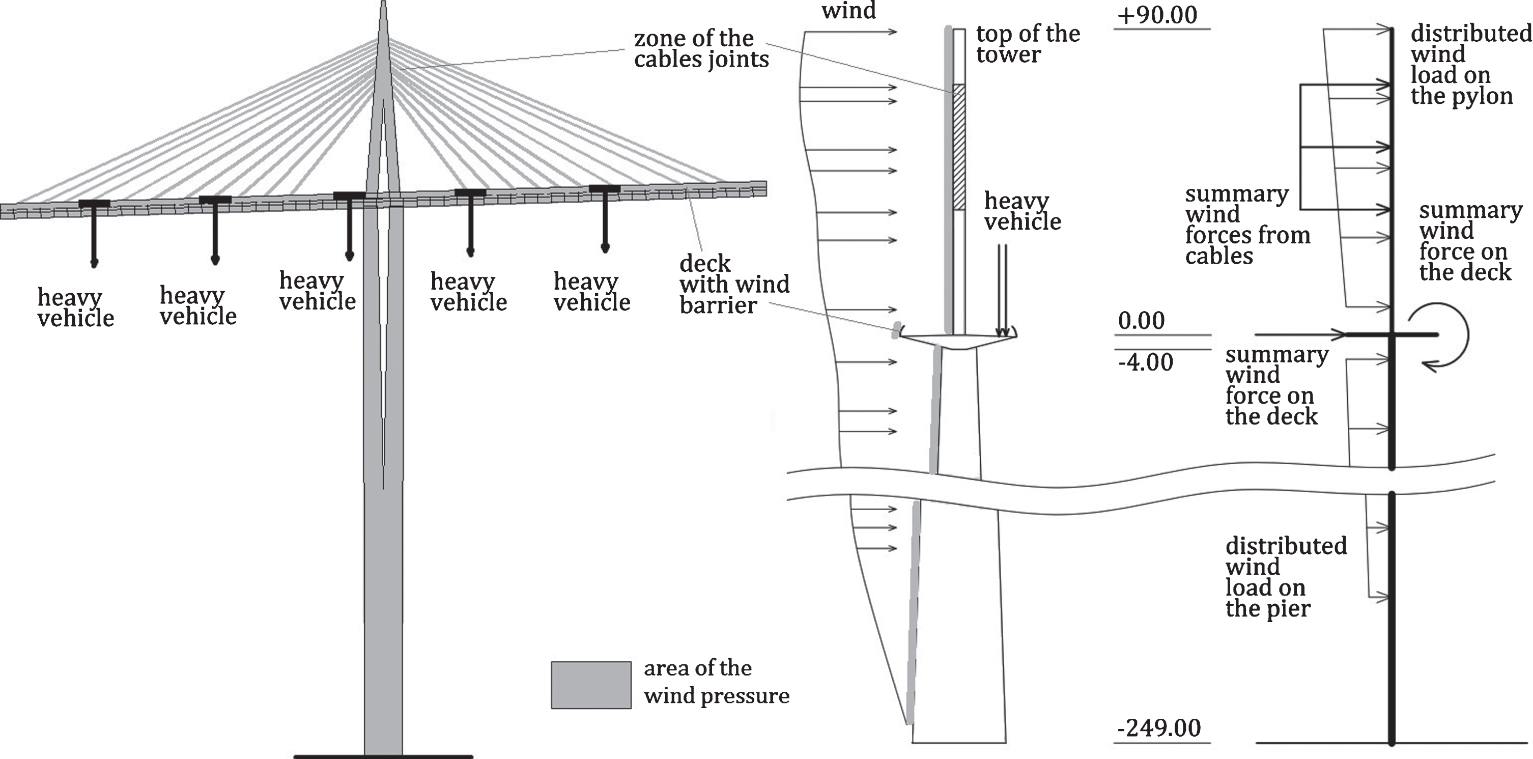
Figure 16 (right) shows how the wind load is transferred from the real 3D model to the 2D computational model. The result wind forces for all the elements of the considered part of the bridge (the pylon, pile, deck, and cables) are shown in Table 8. The wind pressure used in calculations is obtained from the measurements for the known wind velocities at different levels. The reference areas used in calculations correspond to actual dimensions of the studied Millau viaduct. Table 10 in Appendix D shows the values of the bending moments at the deck level of the bridge that are caused by wind forces applied to the 2D computational model for various wind speeds.
Table 6
Combination of extreme wind and extreme traffic actions and probability to their simultaneous occurrence
| Case | Traffic only | Wind only | Combination | ||||
|
|
|
|
|
|
| P (Ωmax > ωmax) | |
| Weekly max, “113” | 8661 | 8.3×10⁻² | 13411 | 5.9×10⁻³ | 22072 | 31809 | 4.8×10⁻⁴ |
| Return level, 120 years | 12450 | 9.5×10⁻⁷ | 167140 | 9.5×10⁻⁷ | 179590 | 267518 | 9.1×10⁻¹³ |
| 5 ”113”, 13 weeks | 12099 | 8×10⁻² | 32524 | 3.5×10⁻⁴ | 44624 | 65120 | 2.8×10⁻⁵ |
| Design, [29] | 176490 | 0.1 per 100 years | 276410 | 0.02 per 1 year | 363056 | 531587 | - |
Table 7
Example of vehicles types
| Type (axles) | Distance between axles (m) | Axle group | Weight of each axle (kN) | |||||||
| 1–2 | 2–3 | 3–4 | 4–5 | 1 | 2 | 3 | 4 | 5 | ||
| 113 (5) | 3.64 | 5.50 | 1.27 | 1.23 | 113 | 15 | 22 | 17 | 17 | 17 |
| 40 (2) | 5.27 | – | – | – | 11 | 41 | 119 | – | – | – |
| 61 (4) | 3.69 | 6.73 | 1.31 | – | 112 | 32 | 139 | 34 | 34 | – |
| 100 (3) | 8.7 | 3.61 | 5.1 | – | 111 | 46 | 65 | 5 | – | – |
| 56 (3) | 6.8 | 1.46 | – | – | 12 | 78 | 142 | 142 | – | – |
Table 8
Wind load as a function of wind speed
| Bridge element | Wind speed (m/s) | Wind pressure (Pa) | Height (m) | Width (m) | Area (m2) | Wind force (kN) | Wind load (kN/m) | Comment |
| Pile, bottom | 28.6 | 528.8 | 155 | 17 | 2635 | 1393 | 9.0 | |
| Pile, top | 31.7 | 647.8 | 90 | 17 | 1530 | 991 | 11.0 | two columns of 8.5 m height |
| Deck | 34.7 | 778.8 | 7 | 342 | 2394 | 1865 | 266.4 | + wind barrier 3 m height |
| Pylon, bottom | 34.7 | 778.8 | 36 | 10 | 360 | 280 | 7.8 | two columns of 5 m height |
| Pylon, | 35.8 | 829.5 | 36 | 8.2 | 295.2 | 245 | 6.8 | |
| Pylon, | 36.9 | 881.7 | 15 | 2.9 | 43.5 | 38 | 2.6 | |
| Cables to pylon | 35.8 | 829.5 | 1330 | 0.5 | 665 | 552 | 27.6 | distributed along 20 m height |
| Cables to deck | 34.7 | 778.5 | 1330 | 0.5 | 665 | 518 | - | from 11 cables |
Table 9
Bending moments for traffic actions and their occurrence
| case | GVW×103 kg | Load (kN) | Bending Moment (kN×m) | Occurrence every |
| Maximum recorded “113” | 86.7 | 850.5 | 7017 | 26 weeks |
| Mean of weekly max | 59.5 | 583.7 | 4815 | 1 week |
| 2×”113” | 66.0 | 647.5 | 5341 | 40 min |
| 3×”113” | 98.1 | 962.4 | 7939 | 12 hours |
| 4×”113” | 116.8 | 1145.8 | 9453 | 2 weeks |
| 5×”113” | 149.5 | 1466.6 | 12099 | 13 weeks |
| RL +CI,single “113″ | 113 + 27 | 1383.2 | 11411 | 120 years |
| RL +CI,5trucks | 565 + 56 | 6092.0 | 50260 | 107 years |
| Design load, [17] | – | LM1 | 176490 | 1000 years |
Table 10
Wind speed and associated wind force applied to the 2D computational model and computed bending moments
| Case | Weekly max | Max recorded | RL, 120 years | Design [9] | ||||
| Wind speed (m/s) | Force (kN) | Wind speed (m/s) | Force (kN) | Wind speed (m/s) | Force (kN) | Wind speed (m/s) | Force (kN) | |
| Pile, bottom | 9.8 | 161.8 | 19.2 | 625.3 | 52.5 | 4691 | 32 | 9544 |
| Pile, top | 12.8 | 162.1 | 22.2 | 488.1 | 55.6 | 3051 | 32 | 5814 |
| Deck | 15.9 | 389.1 | 25.3 | 988.2 | 58.6 | 5313 | 32 | 9097 |
| Pylon, bottom | 15.9 | 58.5 | 25.3 | 148.6 | 58.6 | 799 | 32 | 1368 |
| Pylon, middle | 17.0 | 54.9 | 26.4 | 132.8 | 59.7 | 680 | 32 | 1122 |
| Pylon, top | 18.1 | 9.2 | 27.5 | 21.3 | 60.8 | 104 | 32 | 165 |
| Cables | 17.0 | 123.7 | 26.4 | 299.2 | 59.7 | 1532 | 32 | 2527 |
| Bending moment, | 13411 | 32524 | 167140 | 276410 | ||||
3.5Probabilistic model
Let
(4)
(5)
For weekly duration, for 120 years return level, and for 13 weeks duration, Table 6 displays the probabilities of the extreme wind actions, the extreme traffic actions, and the combination of the simultaneous occurrence of these two extreme actions. Values of the bending moment provided for traffic (Table 9, Appendix D) contribute to the resulting bending moment three times less than the wind. As well, the combination that brings very high values of the bending moment, is probable extremely rare.
3.5.1Design load model
Calculations of design traffic actions Ft are made according to the load model LM1 of European Norms, [18], that consists of two parts: the concentrated axle load FTS and the uniformly distributed load FUDL. Results are shown in the last row of Table 9. According to standards [30], the design value of an action can be crossed in 10% of cases every 100 years in case of traffic on bridges.
The design model for wind actions FW is based on the procedure explained in [9] for the case of wind loads on bridges. Methodology is shortly explained in Annex C, and results are shown in the last row of Table 10. According to standards [30], the design value of an action can be crossed in 2% of cases every year for the wind (as a climatic action).
The design combination of both loads is computed for ultimate limit state (ULS) and serviceability limit state (SLS) respecting formulations proposed in standards [29]. Considering G to be the value of self-weight of the structure and the wind to be a leading action, design combinations Ed can be written as following:
(6)
(7)
where: ψ0 are factors for combination value of accompanying variable traffic actions, ψ0,TS = 0.75 – for the concentrated axle load (LM1, [18]) and ψ0,UDL = 0.4 – for the uniformly distributed load (LM1, [18]). Considering values of partial factors for the wind (γw = 1.5) and traffic (γw = 1.35), Equation (6) and Equation (7) take the following form:
(8)
(9)
Results for combination of extreme wind and extreme traffic actions and probability of their simultaneous occurrence are represented in Table 6. The table shows both, ULS and SLS for each case. In the case of monitored traffic actions, the combination coefficient is taken ψ0 = 1. It can be observed from the table that design values of actions, even using reduction coefficients are much higher than values predicted based on monitoring. This confirms that the structure has extra capacity even in the worth case that can probably arrive during the design operational life.
4Conclusions
The relevance of combining traffic loads with the wind load in the case of cable- stayed bridges is an important question. Even though all unfavorable combinations are considered at the design stage, it is interesting to reanalyze the extreme values combination in a probabilistic framework.
Monitoring of traffic and wind loads at any period of the operational life of a bridge allows for updating the design expected life of the structure. Due to economical and practical reasons, measurements of applied actions are often limited, which require studying the influence of monitoring duration on the quality of results. In order to assess global extreme load effects, a probabilistic approach is proposed in this paper on the base of available data and EVT.
This work has been carried out on the data from the Millau viaduct. Traffic is represented by most frequent types of heavy vehicles and based on BWIM data of 43 days, updated after 176 days of monitoring. Hourly wind data from the weather station near the viaduct have been treated for the same time period. As the combination of both types of loads, their superposition has been carried out.
The analysis that has been made for both wind and traffic actions, proves the efficiency of the POT approach in cases where the number of events for load effects is sufficient to have at least one exceedance of the threshold per day. Moreover, the main drawback of the method — the choice of a threshold — has been addressed. For instance, choice of a threshold value in the MRLP method introduces an uncertainty. Therefore, an updated algorithm (plotting confidence intervals computed for all possible values of a threshold against the threshold with following choosing the best TH with a respect to probabilities of exceedance) is suggested in this study. It shows to be efficient enough and less time-consuming.
The predictions are made for weights of passing vehicles of each type and for wind velocities at different levels of height. The results of obtained approach show that the longer period of monitoring positively influences confidence intervals for long-term predictions. For example, for vehicle weights of the most frequent type, four times longer monitoring duration decreases the value of the confidence interval by 65%.
Another conclusion is the importance of the most frequent type of heavy vehicles as it contributes the most to the entire number of trucks. It means that for long-term extreme events predictions, there are only most frequent of heavy vehicles need to be observed, ignoring frequent light cars, which brings a lot of value, for instance, in the fatigue limit state. This allows for making such type of analysis based on just statistical data that are often available.
In a case of the wind, although it gives good model fitting, the confidence intervals for the return levels are quite high due to the assumption of stationarity of load effects. Predicted wind speeds based on data for the entire life of the Millau viaduct since its opening, do not up-cross the value of 110 km/h that would cause traffic limitations, which allows for assessing probabilities of the combination of extreme cases for both loads as statistically independent variables.
In order to assess the combination of both actions, the part of the bridge containing the highest pylon is studied. Both, wind and traffic actions give bending moments at the level of the deck around its longitudinal axis. The contribution of each load is significantly high, therefore probabilities of occurrence of extreme cases are studied separately and combined together. Single over-weighted trucks (with the weekly mean of around 600 kN) are frequent, however, their contribution to the overall bending moment is not as significant as a passage of a queue of lorries that happen rare enough (twice a month for a group of four or 4 times per year for a queue of five lorries).
The probability calculation that has been carried out, shows that the high values of the bending moment could cause some torsion in the deck with the following consequences on the behavior of trucks with a large trailer, but this event is sufficiently rare.
The further work should include extreme value analysis based on longer statistical data for traffic. The dynamic induced by the wind action should be taken into account for more precise conclusions. Moreover, fatigue of deck elements and cables, which has not been mentioned here, could be considered as it can bring contribution to the reliability level of the structure.
Conflict of interest
None to report.
Appendices
Appendix
Abbreviations
EVT | Extreme Value Theory |
POT | Peaks Over Threshold |
BWIM | Bridge-Weigh-In-Motion |
GPD | Generalized Pareto Distribution |
LE(s) | Load Effect(s) |
MRLP | Mean Residual Life Plot |
RL(s) | Return Level(s) |
CI(s) | Confidence Interval(s) |
BM(s) | Bending Moment(s) |
PE | Probability of Exceedance |
SHM | Structural Health Monitoring |
BMS | Bridge Management System |
GVW | Gross Vehicle Weight |
ULS | Ultimate Limit State |
SLS | Serviceability Limit State |
LM | Load Model |
A. Peaks over threshold approach
This approach has been recently proved to be a good solution for predictions of extreme traffic actions [8, 31]. As a time-series process, peak values of LEs, that lay above a certain threshold, are fitted to the GPD (Fig. 11).
Let X = (X1, …, Xi, …, Xn) to be the sequence of random variables representing
LEs with the distribution function. Let Y = (Y1, …, Yj, …, Ym) to be the sequence of random variables representing exceedances of a threshold u and defined by Y = X - u, for every threshold excess Xj ∈ X so that Xj > u. A few assumptions have to be made for the application of the EVT:
• identical distribution of random variables Xi,
• random variables Xi are independent,
• threshold u is sufficiently high.
The cumulative distribution function Fu of Yj, can be expressed as:
(10)
The main principle of the POT approach is described a few decades ago [32] and it is based on the following expression: Fu(Yj) tends to the upper tail of a GPD, Equation (11), with shape and scale parameters (σ and ξ). Certain conditions have to be respected in order to apply this approach: i) Yj = Xi – u≥0, ii) Xi≥u for ξ≥0 and u ⩽ Yj ⩽ u - σ/ - ξ for ξ < 0, iii) σ > 0.
(11)
For a long period, observations can be based on the cumulative distribution function of extreme values over a shorter period [33]. Provided, for instance, in [3], for the probability Pr [X ⩽ Xi|Xi > u] with the probability of exceedance ζu = Pr{ Xj > u }, the solution to the function is the following:
(12)
B. Confidence intervals
The means of comparison between several load cases in this paper is the value of the statistical uncertainty represented by CIs for RLs. Here, 95% confidence intervals are used for return levels and they depend on the value of variance:
(13)
The variance is assessed here based on the delta method [35] and given by:
(14)
The value of variance for RL depends on variance of GPD parameters ξ, σ and on probability of exceedance ζu. All three parameters have maximum likelihood estimates:
(15)
If vi,j represents values of variance-covariance matrix of GPD parameters ξ and σ, the complete variance-covariance matrix for all parameters is found as:
(16)
For a p -observations RL Equation (17) gives the
(17)
It was recently concluded [36] that the efficiency of the described method is high enough under the assumption of normal distribution of return levels estimators. Therefore, it is used further in the current research.
C. Design values of wind force
The general expression of a wind force Fw acting on a structure:
(18)
Where:
ρ is the air density, ρ = 1.25 kg m-3 is the recommended value,
νb is the basic wind velocity, see Equation (22),
ce is the exposure factor, that can be found from Equation (19),
cf is the force coefficient wind actions on bridge decks in the x-direction, recommended value cf = 1.3),
Aref the reference area reference area of all the elements of the considered part of the bridge (the pylon, pile, deck, and cables) correspond to actual dimensions of the studied Millau viaduct.
(19)
where:
Vm is the mean wind velocity at a height z above the ground, see Equation (21).
Iv (z) is the turbulence intensity at height z:
(20)
K1 is the turbulence factor, recommended value is 1.0,
co(z) is the oreography factor,
Z0 is the roughness length. The mean wind velocity:
(21)
where:cr (z) = 0.19 (z0/ - z0,II) 0.07 × ln (z/ - z0) is the roughness factor with z0 - the roughness length, z0 = z0,II = 0.05m in the case of Millau, zmin = 2 m.
The basic wind velocity:
(22)
νb,0 is the fundamental value of the basic wind velocity, defined as the characteristic 10 minutes mean wind velocity at 10 m above ground level in open country with low vegetation and few isolated obstacles (distant at least 20 obstacle heights), in the area of Millau the value νb,0 = 24 m/ - s as it is stated in National Annex, [9].
cdir and cseason are directional and seasonal factors, with recommended values 1.0.
cprob is a probability factor that should be used as the return period for the design of the Millau viaduct defers from T = 50 years. Considering a 2-% value of annual probability of exceedance, parameters K = 0.2 and n = 0.5, then, cprob = 1.33
D. Calculations
Supporting information on the computational process for traffic and wind actions can be found in the following tables:
Acknowledgments
This project has received funding from the European Union Horizon 2020 research and innovation programme under the Marie Sklodowska-Curie grant agreement No 676139. The grant is gratefully acknowledged.
The BWIM measurements for the Millau viaduct were obtained with the help from CESTEL, Slovenia and EIFFAGE, France, which is highly appreciated.
References
[1] | Dissanayake PBR , Karunananda PAK . Reliability Index for Structural Health Monitoring of Aging Bridges. Structural Health Monitoring: An International Journal. (2008) ;7: :175–83. doi: 10.1177/1475921708090555. URL http://journals.sagepub.com/doi/10.1177/1475921708090555. |
[2] | Kuhn B . Assessment of Existing Steel Structures Recommendations for Estimation of the Remaining Fatigue Life. Procedia Engineering. (2013) ;66: :3–11. ISSN 18777058. doi: 10.1016/j.proeng.2013.12.057. URL http://linkinghub.elsevier.com/retrieve/pii/S1877705813018900. |
[3] | Coles S . An Introduction to Statistical Modeling of Extreme Values. Springer Science & Business Media, August (2001) . ISBN 978-1-85233-459-8. |
[4] | Agarwal P , Manuel L . Simulation of offshore wind turbine response for long-term extreme load prediction. Engineering Structures. (2009) ;31: (10):2236–46. ISSN 0141-0296. doi: 10.1016/j.engstruct. URL http://www.sciencedirect.com/science/article/pii/S0141029609001436. |
[5] | Roth M , Buishand TA , Jongbloed G , Klein Tank AMG , van Zanten JH . Projections of precipitation extremes based on a regional, non-stationary peaks-over-threshold approach: A case study for the Netherlands and north-western Germany. Weather and Climate Extremes. (2014) ;4: (Supplement C):1–10. ISSN 2212-0947. doi: 10.1016/j.wace.2014.01.001. URL http://www.sciencedirect.com/science/article/pii/S2212094714000024. |
[6] | Sigauke C , Bere A . Modelling non-stationary time series using a peaks over threshold distribution with time varying covariates and threshold: An application to peak electricity demand. Energy. (2017) ;119: (Supplement C):152–66. ISSN 0360-5442. doi: 10.1016/j.energy.2016.12.027. URL http://www.sciencedirect.com/science/article/pii/S0360544216318321. |
[7] | Treacy MA , Brhwiler E , Caprani CC . Monitoring of traffic action local effects in highway bridge deck slabs and the influence of measurement duration on extreme value estimates. Structure and Infrastructure Engineering. (2014) ;10: (12):1555–72. ISSN 1573-2479. doi: 10.1080/15732479.2013.835327. |
[8] | Zhou XY . Statistical analysis of traffic loads and their effects on bridges. PhD Thesis, University Paris-Est, May 2013. URL https://tel.archives-ouvertes.fr/tel-00862408/document. |
[9] | EN 1991-1-4: Eurocode 1: Actions on structures - Part 1–4: General actions - Wind actions. European Committee for Standardization, 2005. URL http://archive.org/details/en.1991.1.4.2005. |
[10] | Arena A , Lacarbonara W , Valentine DT , Marzocca P . Aeroelastic behavior of long-span suspension bridges under arbitrary wind pro- files. Journal of Fluids and Structures. (2014) ;50: :105–19. ISSN 08899746. doi: 10.1016/j.jfluidstructs.2014.06.018. URL http://linkinghub.elsevier.com/retrieve/pii/S0889974614001364. |
[11] | Zhang W , Cai CS , Pan F , Zhang Y . Fatigue life estimation of existing bridges under vehicle and non-stationary hurricane wind. Journal of Wind Engineering and Industrial Aerodynamics. (2014) ;133: (Supplement C):135–45. ISSN 0167-6105. doi: 10.1016/j.jweia.2014.06.008. URL http://www.sciencedirect.com/science/article/pii/S0167610514001159. |
[12] | Davenport AG . The generalization and simplification of wind loads and implications for computational methods. Journal of Wind Engineering and Industrial Aerodynamics. (1993) ;46: :409–17. |
[13] | Mikosch T , Embrechts P , Kluppelberg C . Modelling Extremal Events for Insurance and Finance. Springer Verlag Berlin Heidelberg, February (2012) . |
[14] | Rudiger Frey Alexander J. McNeil, Embrechts P. Quantitative Risk Management: Concepts, Techniques, and Tools. Princeton University Press, September (2005) . |
[15] | Haugen T , Levy JR , Aakre E , Tello MEP . Weigh-in-Motion Equipment Experiences and Challenges. Transportation Research Procedia. (2016) ;14: :1423–32. ISSN 23521465. doi: 10.1016/j.trpro.2016.05.215. URL http://linkinghub.elsevier.com/retrieve/pii/S2352146516302174. |
[16] | Richardson J , Jones S , Brown A . On the use of bridge weigh- in-motion for overweight truck enforcement. International Journal of Heavy Vehicle Systems. (2014) ;21: :83–104. |
[17] | Cachot E , Vayssade T , Virlogeux M , Lancon H , Hajar Z , Servant C . The Millau Viaduct: Ten Years of Structural Monitoring. Structural Engineering International. (2015) ;25: :375–380. doi: 10.2749/101686615x14355644770776. URL http://www.ingentaconnect.com/content/10.2749/101686615X14355644770776. |
[18] | EN 1991-1-2: Eurocode 1: Actions on structures - Part 2: Traffic loads on bridges. European Committee for Standardisation, (2003) . |
[19] | Buonomo M , Servant C , Virlogeux M , Cremer J-M . The design and the construction of the Millau Viaduct. Steelbridge. (2004) , 2004. |
[20] | OBrien EJ , Enright B . Modeling same-direction two-lane traffic for bridge loading. Structural Safety. (2011) ;33: (4):296–304. ISSN 0167-4730. doi: https://doi.org/10.1016/j.strusafe.2011.04.004. URL http://www.sciencedirect.com/science/article/pii/S0167473011000427. |
[21] | Caprani CC , Obrien EJ , Lipari A . Long-span bridge traffic loading based on multi-lane traffic micro-simulation. Engineering Structures. (2016) ;115: :207–19. ISSN 0141-0296. doi: https://doi.org/10.1016/j.engstruct.2016.01.045. URL http://www.sciencedirect.com/science/article/pii/S0141029616000614. |
[22] | Schmidt F , Jacob B , Servant C , Marchadour Y . Experimentation of a bridge WIM system in France and applications for bridge monitoring and overload detection. In International Conference on Weigh-In-Motion ICWIM6, (2012) ;8. France. URL https://hal.archives-ouvertes.fr/hal-00950245. |
[23] | Alcover IF . Data-based models for assessment and life prediction of monitored civil infrastructure assets. PhD thesis, University of Surrey, January 2014. URL http://epubs.surrey.ac.uk/807811/. |
[24] | Code de la route - Article R312-4, (2018) . |
[25] | Sylvestre G , Herv L . Dix annees de monitoring structurel du viaduc de Millau. Travaux (Paris), (2013) ;(896):108–17. ISSN 0041-1906. http://www.refdoc.fr/Detailnotice?idarticle. |
[26] | Kree P , Soize C . Mathematics of Random Phenomena: Random Vibrations of Mechanical Structures (Mathematics and Its Applications). Springer, (1986) . |
[27] | Cremona C . Structural Performance: Probability-based Assessment. John Wiley & Sons, Inc., Hoboken, NJ, USA, February 2013. ISBN 978-1-118-60117-4 978-1-84821-236-7. URL http://doi.wiley.com/10.1002/9781118601174. DOI: 10.1002/9781118601174 |
[28] | Bommier E . Peaks-over-threshold modelling of environmental data. Master’s thesis, Uppsala University, Applied Mathematics and Statistics, (2014) . |
[29] | Massey FJ . The kolmogorov-smirnov test for goodness of fit. Journal of the American Statistical Association. (1951) ;46: :68–78. |
[30] | EN 1990: Eurocode: Basis of structural design. European Committee for Standardisation, (2002) . |
[31] | Zhou X-Y , Schmidt F , Toutlemonde F , Jacob B . A mixture peaks over threshold approach for predicting extreme bridge traffic load effects. Probabilistic Engineering Mechanics. (2016) ;43: (Supplement C):121–31. ISSN 0266-8920. doi: 10.1016/j.probengmech.2015.12.004. URL http://www.sciencedirect.com/science/article/pii/S0266892015300680. |
[32] | Pickands J . Statistical Inference Using Extreme Order Statistics. The Annals of Statistics. (1975) ;3: (1):119–31. ISSN 0090-5364. URL http://www.jstor.org/stable/2958083. |
[33] | Crespo-Minguilln C , Casas JR . Structural Safety. A comprehensive traffic load model for bridge safety checking. (1997) ;19: (4):339–59. ISSN 0167-4730. doi: 10.1016/S0167-4730(97)00016-7. URL http://www.sciencedirect.com/science/article/pii/S0167473097000167. |
[34] | Obrien EJ , Schmidt F , Hajializadeh D , Zhou B , Enright X-Y , Caprani CC , Wilson S , Sheils E . A review of probabilistic methods of assessment of load effects in bridges. Structural Safety. (2015) ;53: :44–56. |
[35] | Hosking JR , Wallis JRM . Parameter and quantile estimation for the generalized pareto distribution. Technometrics. (1987) ;29: :339. |
[36] | Schendel T , Thongwichian R . Confidence intervals for return levels for the peaks-over-threshold approach. Advances in Water Resources. (2017) ;99: :53–9. ISSN 03091708. doi: 10.1016/j.advwatres.2016.11.011. URL http://linkinghub.elsevier.com/retrieve/pii/S0309170816306960. |


