
Reliability of bridge decks in the United States
Abstract
Deterioration of bridge decks in the United States is an important issue due to its major impact on bridge maintenance costs nationwide. In this paper, results of survival (reliability) analyses performed on bridge data for all fifty states and Puerto Rico are presented. Data were obtained from the 2011 National Bridge Inventory (NBI) database. The end of service life is defined as a recorded NBI bridge deck rating of 5. Only non-reconstructed bridges and conventional bridge types and decks were considered. The NBI-derived parameters included in the analyses were age, average daily traffic (ADT), deck surface area, and deck rating. Each state’s data were analyzed separately to assess and compare relative performance among the states. Deck reliability at an age of fifty years ranges from less than 20% to over 90% . The geographic regions with the highest overall 50-year reliability are generally in the northeastern and northern United States.
1Introduction
1.1Background
Deterioration of bridge decks in the United States is a national concern due to the high costs of repair and rehabilitation. In the northern states where common deicing salts (e.g. sodium chloride) are used to melt ice on roads during winter, corrosion of reinforcing bars and subsequent cracking and spalling of concrete decks is a major issue. Long-term penetration of chloride ions into concrete eventually results in corrosion of steel and cracking of the surrounding concrete. In coastal areas of the United States, exposure to salt-laden air and seawater results in chloride-induced damage to reinforced concrete bridge elements. Other modes of deterioration of concrete include freeze-thaw damage, alkali-silica reactivity, carbonation, etc.
Reliable information on the timing of the end of service life, whether for general consideration (system wide) or for specific bridges, would be extremely valuable for long-term planning and implementation of bridge deck maintenance and repair. A number of researchers have developed theoretical and analytical models for corrosion-induced deterioration of bridge decks [7, 9, 13]. However, such analytical models require a number of assumptions regarding concrete properties, chloride diffusion parameters, chloride thresholds for corrosion initiation, and timing of crack initiation and propagation. The overall validity of such models must also be verified with actual long-term performance data.
On the other hand, conventional structural reliability models are typically based on assessments of the likelihood of failure in the form of applied loads exceeding structural resistance [3, 5, 10, 11]. Reliability models that are based on strength limit states can also be time-dependent, with the influence of time considered on the resistance and/or the loads. Strength-based reliability analyses form the basis for the Load and Resistance Factor Design (LRFD) used in the AASHTO [1] Bridge Design Specifications. However, the primary mode of long-term failure in bridge decks is not based on structural failure (flexural, beam shear, or punching shear). Such end of service life is mostly related to serviceability issues such as corrosion-induceddeterioration.
Survival models (or “time-to-event” models) are commonly used in medical and biomedical research as well as other applications to assess the influence of various parameters on the timing of particular events (such as survival time of cancer patients after administration of new drugs, etc.). In this approach, typically large-scale data are analyzed to develop statistical models that consider the influences of contributing parameters on the timing of outcomes. These models are not based on assessing the likelihood of one parameter exceeding another (e.g. loads exceeding resistance). Also, survival models do not attempt to address theoretical/technical reasons why one parameter may work better than others. This approach can however assess whether individual parameters are in fact affecting the timing of the outcome. Survival models have been used in bridge engineering applications but their use is not widespread. Examples include works by Yang et al. [17] and Beng and Matsumoto [4].
The existence of a comprehensive database of bridge information in the United States, the National Bridge Inventory (NBI) database, provides the necessary large-scale source of data for such an effort across all states. The NBI database includes basic bridge information as well as numerical ratings given by bridge inspectors (on a typically biannual basis) to major bridge components including decks. In the following sections, more information on NBI records and the process of extracting the data used in the study are presented.
In a preceding study, Tabatabai et al. [12] developed a survival model for bridge decks in Wisconsin using data from the 2005 NBI records. A recorded deck rating of 5 (on a scale of 0 to 9) was considered to be the end of service life for a bridge deck. The following NBI data were extracted for bridges with a deck rating of 5: age of bridge, Average Daily Traffic (ADT), deck surface area, and type of superstructure (steel or concrete). Data from bridges with common superstructures types and conventional reinforced concrete decks were considered only (i.e. uncommon superstructure types such as cable-stayed bridges or steel decks were excluded). Reconstructed bridges were also excluded from the analyses. Four different survival models were considered and fit to the extracted NBI data for Wisconsin. These four models consisted of Weibull, log-logistic, lognormal, and hypertabastic [12]. The hypertabastic accelerated failure time model was determined to be the best-fit model based on the Akaike Information Criterion (AIC) [2]. This model was therefore used to analyze bridge deck data from all fifty states plus Puerto Rico in the study reported here.
1.2Objective and scope
The objective of this study was to develop statistical models for time-dependent bridge deck reliability (survival) and failure rate (hazard) for all fifty states and Puerto Rico. Data necessary to accomplish this work were extracted from the 2011 NBI records. The factors considered were deck rating, bridge age, ADT, and deck surface area.
The overall approach used by Tabatabai et al. [12] for the analysis of Wisconsin bridge deck data was also used in this study. Data from each state were analyzed separately. A comparison of reliability results among the states reflects their differing climatic and exposure conditions as well as varying design and maintenance practices.
To have a common basis for comparisons, reliability and failure rates were calculated and presented when covariates (deck area and ADT) were either equal to the national median or equal to each state’s own median values.
2Development of survival models
2.1NBI data and parameter selections
Bridges in the United States are generally inspected once every two years, at which time the inspectors give numerical ratings to various major components of the bridge such as bridge decks. These ratings are typically based on visual observations of damage in the form of cracking, spalling or other signs of distress. NBI numerical ratings range from “failed condition” (0) to “excellent condition” (9). A recorded deck rating of 5 (“fair condition”) is considered to be the end of service life in this study. Many regard a deck rating of 5 or 4 as the time when minor or major repairs are required [6]. A bridge becomes “structurally deficient” if it has a deck rating of less than 5.
Tabatabai et al. [12] provide a detailed description of the extraction procedures for the NBI data used in their study (as well as this study). A summary of this data extraction process is discussed here. As a first step, all NBI records with missing parameters of deck rating, construction date, or ADT were excluded from consideration. Next, bridges with records of previous reconstruction or rehabilitation as well as those with less common superstructure types and decks were removed from consideration. Only conventional concrete, prestressed concrete and steel superstructures were considered (i.e. truss, arch, or cable-stayed bridges were not included). Finally, only bridges with conventional decks (cast-in-place or precast concrete) were retained.
The following parameters were included in the analyses: 1) deck rating (NBI Item 58); 2) age (NBI Item No. 90, year of last inspection minus Item No. 27, year built); 3) deck area (Item No. 49, structure length times Item No. 51, curb-to-curb width); and 4) ADT (Item No. 29). The parameters selected were chosen because they have potential relevance to long-term reliability of bridge decks. The NBI parameter ADTT (Average Daily Truck Traffic) was not used in the analyses. The AASHTO LRFD Standard Specifications for Highway Bridges [1] provide conversion factors that relate ADTT to ADT on rural and interstate highways. Because of this correlation, only one of the two parameters could be used in the analyses as an independent parameter. ADT was chosen because service life of decks is typically a serviceability concern and not a structural failure issue. Deck surface area was included as a parameter because larger deck surfaces are expected to have higher likelihood of developing defects.
In preceding studies [8, 12], the type of superstructure (steel or concrete) was also included as a parameter. However, the type of superstructure had an inconsistent effect on deck reliability in the six northern states that were studied using this approach [8]. Therefore, this parameter was not included in the fifty-state study. Other parameters in the NBI database were not considered (such as location, features intersected, bridge clearances, structure length ...) as they were considered to be either not related (directly or indirectly) to deck performance, or they were considered to be correlated with one of the parameters thatwere included.
The data from various states were analyzed separately (not combined). Thus comparisons of reliability results among various states would include the effects of their differing climatic and environmental conditions, maintenance practices, deicing procedures, etc. The hypertabastic accelerated failure time model was used for the analyses reported here.
2.2Hypertabastic survival model
Reliability or survival (S) is defined as the probability of not reaching the end of service life at a given age (1 minus the probability of failure - reaching the end of service life). Instantaneous failure rate or hazard (h) is defined as the probability of failure per unit time at any given time (age) assuming that failure did not occur prior to that time.
The hypertabastic statistical distribution was first introduced by Tabatabai et al. [16]. The hypertabastic distribution has been used in biomedical applications such as studies of survival of cancer patients [14, 15]. An important advantage of the hypertabastic hazard function compared to other such distributions (e.g. Weibull, log-logistic, lognormal ...) is its flexibility in representing a variety of different shapes of the hazard (failure rate) function [12, 16]. These hazard shape patterns could include increasing followed by decreasing with time, increasing towards an asymptote, monotonically decreasing with time, increasing with upward concavity followed by increasing with downward concavity, increasing with upward concavity followed by a linear increase, or continuous increasing with upward concavity [12, 16].
The theoretical basis and complete equations for the hypertabastic model is given in Tabatabai et al. [12]. Therefore, in this paper, only the equations needed to calculate reliability and failure rates are provided:
(1)
(2)
(3)
(4)
3Results
3.1ADT and deck areas
Table 1 shows median and mean values for ADT and deck area in each state as well as the entire United States. To obtain more representative results for these ADT and deck area values, the data used in conjunction with Table 1 results were not restricted to bridges with a deck rating of 5 alone. Instead, bridge records associated with all deck ratings were used. In general, there are substantial differences between mean and median ADT and deck area values in all states. This indicates the overall influence of bridges with extremely large ADT and deck area values. The median ADT and deck area for the entire United States are 1703 vehicles and 355.3 m2, respectively. The corresponding mean values are substantially higher at 9687 vehiclesand 755.9 m2.
3.2Age of bridges with a deck rating of 5
Table 2 shows the mean, median, and standard deviation for age of bridges (in years) with a deck rating of 5. These ages are not direct indicators of comparative reliability since they are influenced by varying parameters of ADT and deck area. The median age of bridges for various states range from 38 to 74 years with an overall (United States) median of 50.0 years.
3.3Parameters α, β, c, and d
The method of maximum likelihood was used to determine parameters α, β, c, and d that are used in Equations 1 through 4. The resulting parameters for each state are shown in Table 3. These parameters along with Equations 1 and 2 can be used to estimate reliability and failure rate for any state and at the desired age, deck area, and ADT.
3.4Reliability and failure rate
Using Equations 1 and 2 and parameters shown in Table 3, the reliability and failure rates for each of the fifty states and Puerto Rico were determined using two sets of covariate (ADT and deck area) values. The first set of covariates were set equal to the median national (United States) values of ADT (1703 vehicles) and deck area (355 m2). A common set of covariates would allow a direct comparison of bridge deck reliability and failure rates across all states without the influence of ADT and deck area. Any differences noted would then be related to other factors including climatic conditions, design and maintenance practices, deicing practices (if any), construction quality control, etc. (but not ADT and deck area). The second set of covariates were set equal to the median ADT and deck area values for each state. Results from the second set of covariates compare reliability and failure rates among different states considering various states’ differing ADT and deck areas in addition to all of the other factors described above.
Table 4 shows reliability and failure rate results at age 50 for both set of covariates in a tabular form. Vermont, Hawaii, and Maine show the highest reliability for both sets of covariates. On the other hand, Wyoming, California, and Nebraska show the lowest reliabilities (at age 50) for both sets of covariates. Figure 1 shows the 50-year reliability results on a map of the United States with ADT and deck area equal to the national median values. Although variations exist, the states with the highest deck reliabilities are generally more prevalent in the northeastern and northern regions. States in the southwestern and western regions generally show the lowest 50-year reliability. This is somewhat surprising given the fact that the northern regions suffer from more severe winters, and deicing salts are routinely and extensively used to melt ice and snow in wintertime. Further research is needed to assess the contributing factors that result in such differences.
Equations 1 and 2 and the parameters of Table 3 can also be used to determine reliability and failure rates at other ages, ADT levels, and deck areas. Graphs of reliability, failure rate and probability density function (pdf) can be plotted for each state as described by Tabatabai et al. [12]. Figures 2, 3 and 4 show reliability, failure rate, and pdf graphs for six major states of California, Texas, Florida, New York, Michigan, and Washington State, respectively.
3.5P-values
A set of p-values are calculated for each state and covariate during the analyses. Table 5 shows the calculated p-values. These p-values indicate whether a particular covariate is statistically significant. In general, a small p-value (e.g. less than 0.02) for a covariate in a particular state indicates that the covariate is a statistically significant parameter for that state. Although there are a few states with p-values higher than 0.02 for one or both covariates, the great majority of states’ results indicate that both deck area and ADT are statistically significant parameters.
4Summary and conclusions
Survival analyses were performed on bridge deck data from all fifty states and Puerto Rico to assess long-term bridge deck reliability and failure rates in various states. The 2011 National Bridge Inventory database was used to obtain data on deck rating, bridge age, average daily traffic, and deck area. A recorded deck rating of 5 was selected as the end of service life for the bridge deck. The hypertabastic accelerated failure time model was used for the analyses, and model parameters were determined using the maximum likelihood approach. Each state’s data were analyzed separately so that relative performance among the states could be assessed.
The national median bridge age at the end of deck service life is 50.0 years with a standard deviation of 19.5 years. Deck reliability at an age of fifty years varies from state to state, ranging from less than 20% to over 90% . The geographic regions with the overall highest reliability at an age of 50 years are in the northeastern and northern United States. In general, the lowest reliabilities were obtained for states in the southwestern and western United States. Although corrosion issues are more prevalent in the northern regions because of the widespread use of deicing chemicals, the bridge deck reliabilities are higher in those same regions. Further studies are needed to effectively and conclusively determine the reasons behind these variations, which may be possibly related to differing design, construction and maintenance practices resulting from differing perceived risk or hazard.
In most states, the reliability of bridge deck at 75 years is less than 15% (when covariates are at national median levels). The shapes of the failure rate function with time also varies from state to state. In general, there is a continuous rise in failure rates with time. However, in some states, the rate of increase in failure rate is reduced at approximately 30 years of age.
References
1 | AASHTO(2010) LRFD bridge design specifications5th editionAmerican Association of State Highway and Transportation Officials |
2 | Akaike A(1974) New look at statistical model identificationIEEE Transactions on Automatic Control19: 6716723IEEE |
3 | Akgul F, Frangopol DM(2004) Bridge rating and reliability correlation: Comprehensive study for different bridge typesJournal of Structural Engineering130: 710631074ASCE |
4 | Beng S, Matsumoto T(2012) Survival analysis on bridges for modeling bridge replacement and evaluating bridge performanceJournal of Structure and Infrastructure Engineering8: 3251268 |
5 | Estes AC, Frangopol DM(2005) Load rating versus reliability analysisJournal of Structural Engineering131: 5843847ASCE |
6 | Hearn G. Bridge management systems. In: Frangopol, D.M. (ed.). Bridge Safety and Reliability, Chapter 8 1999 |
7 | Lee C-W. Simulations of long-term bridge deck deterioration due to corrosion. PhD Dissertation: University ofWisconsin – Milwaukee, 2011 |
8 | Lee C-W, Tabatabai H, Tabatabai MA(2015) Bridge deck survival analyses for six northern states of the United States. Paper Submitted for publication. University of Wisconsin – Milwaukee |
9 | Liu Y, Weyers RE(1998) Modeling the time-to-corrosion cracking in chloride contaminated reinforced concrete structuresACI Materials Journal95: 6675681American Concrete Institute |
10 | Morcous G, Akhnoukh A(2007) Reliability analysis of NU girders designed using AASHTO LRFDProceedings of the Structures CongressASCE |
11 | Nowak AS, Eamon CD(2008) Reliability analysis of plank decksJournal of Bridge Engineering13: 5540546ASCE |
12 | Tabatabai H, Tabatabai MA, Lee C-W(2011) Reliability of bridge decks in wisconsinJournal of Bridge Engineering16: 15362ASCE |
13 | Tabatabai H, Lee C-W(2006) Simulation of bridge deck deterioration caused by corrosionIn: Proceedings of corrosion paper 06345, San Diego, CA: National Association of Corrosion Engineers (NACE) |
14 | Tabatabai MA, Eby W, Nimeh N, Singh K(2012a) Role of metastasis in hypertabastic survival analysis of breast cancer. Interactions with clinical and gene expression variablesCancer Growth nd Metastasis5: 117 |
15 | Tabatabai MA, Eby W, Nimeh N, Singh K, Li H(2012b) Clinical and multiple gene expression variables in survival analysis of breast cancer: Analysis with the hypertabastic survival modelBMC Medical Genomics5: 6310.1186/1755-8794-5-63 |
16 | Tabatabai MA, Zoran B, Williams DK, Singh KP(2007) Hypertabastic survival modelTheoretical Biology and Medical Modeling4: 40 |
17 | Yang Y, Kumaraswamy M, Pam H, Xie H(2013) Integrating semiparametric and parametric models in survival analysis ofbridge element deteriorationJournal of Infrastructure Systems19: 2176185ASCE |
Figures and Tables
Fig.1
Bridge deck reliability in various states at the age of 50 years – ADT and deck area at national median values.
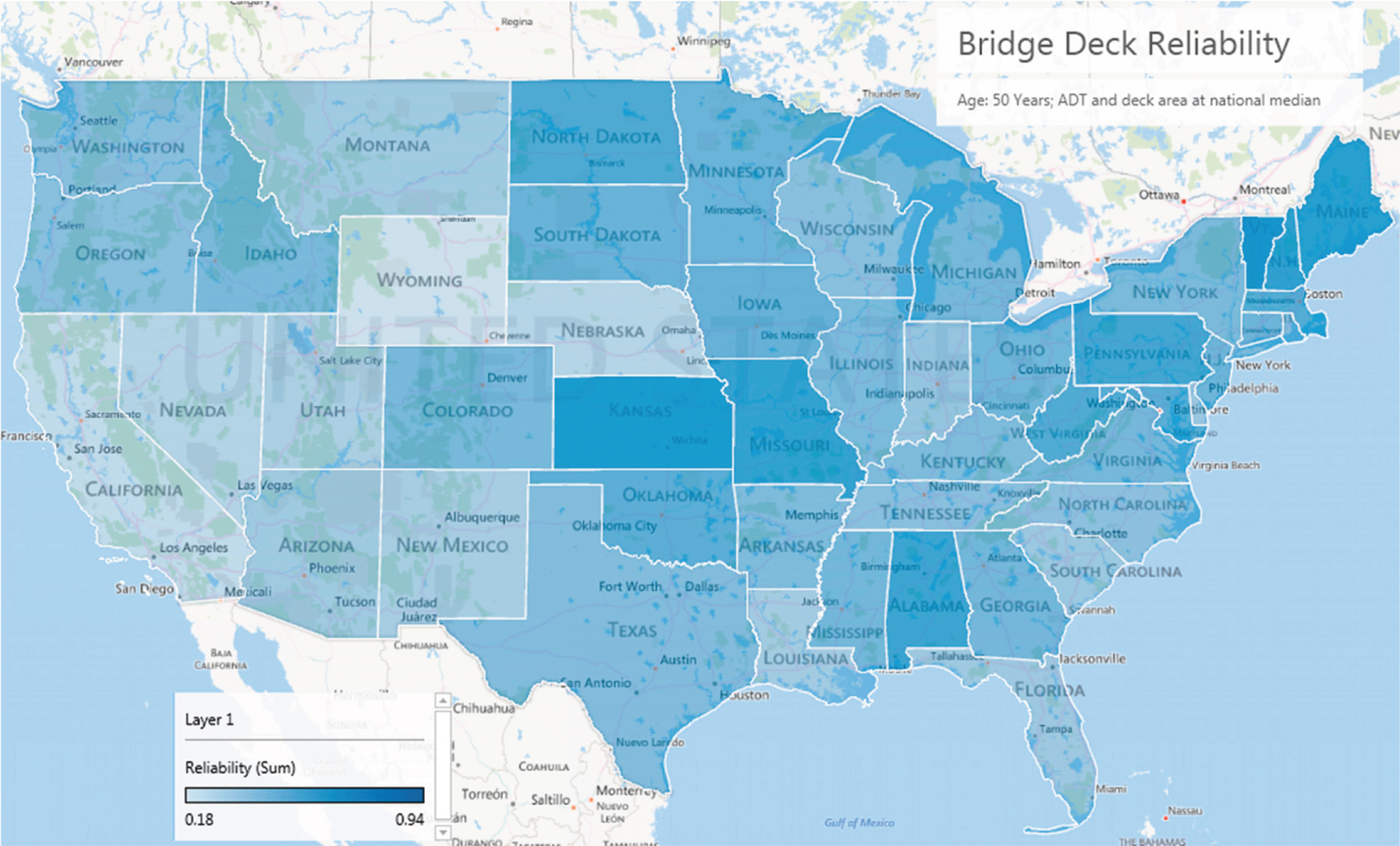
Fig.2
Variation of deck reliability with age for Washington State, California, Michigan, Florida, Texas, and New York with ADT and deck areas at national median (ADT = 1703 and deck area = 355.3 m2).
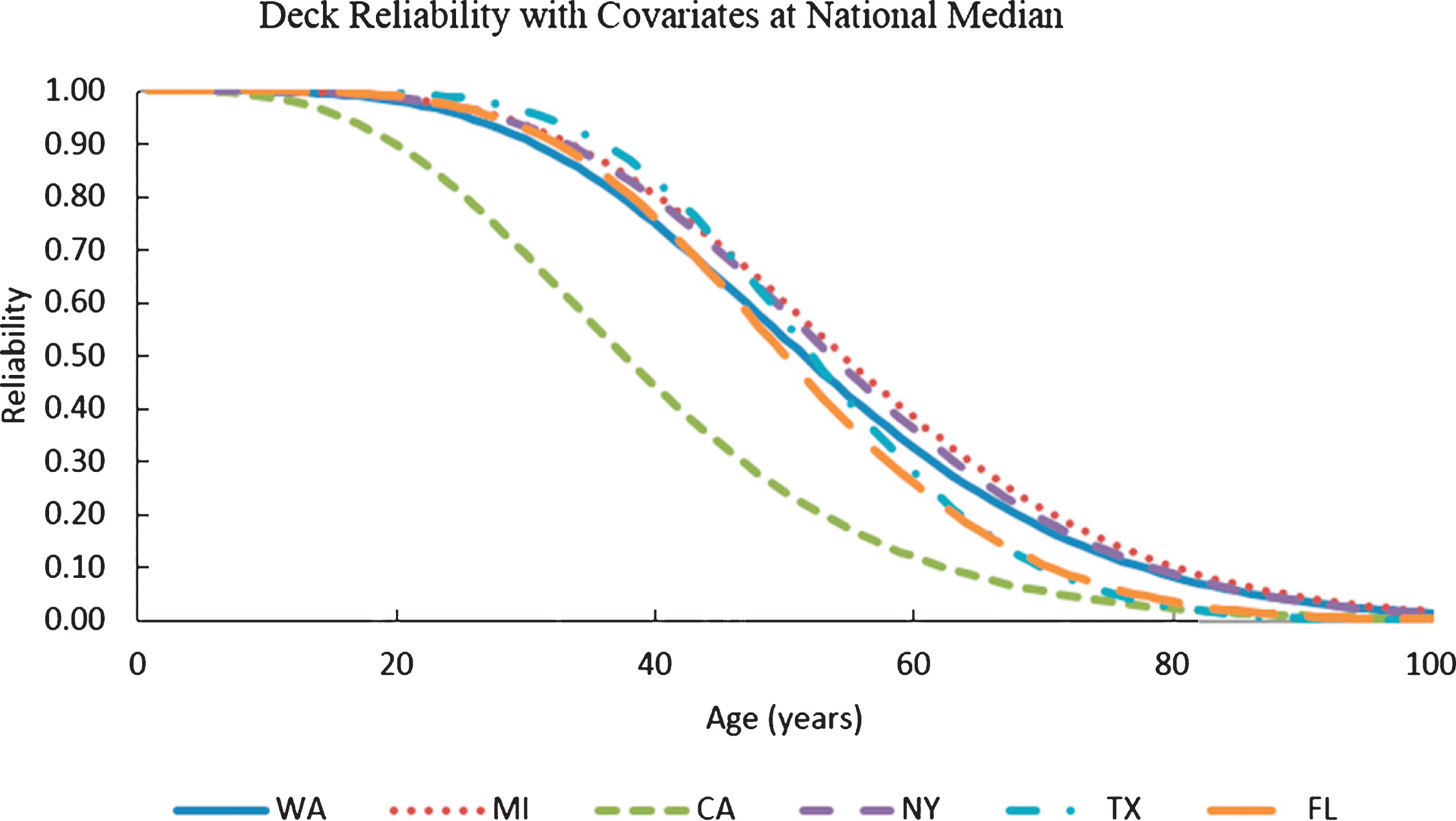
Fig.3
Variation of deck failure rates with age for Washington State, California, Michigan, Florida, Texas, and New York with ADT and deck areas at national median (ADT = 1703 and deck area = 355.3 m2).
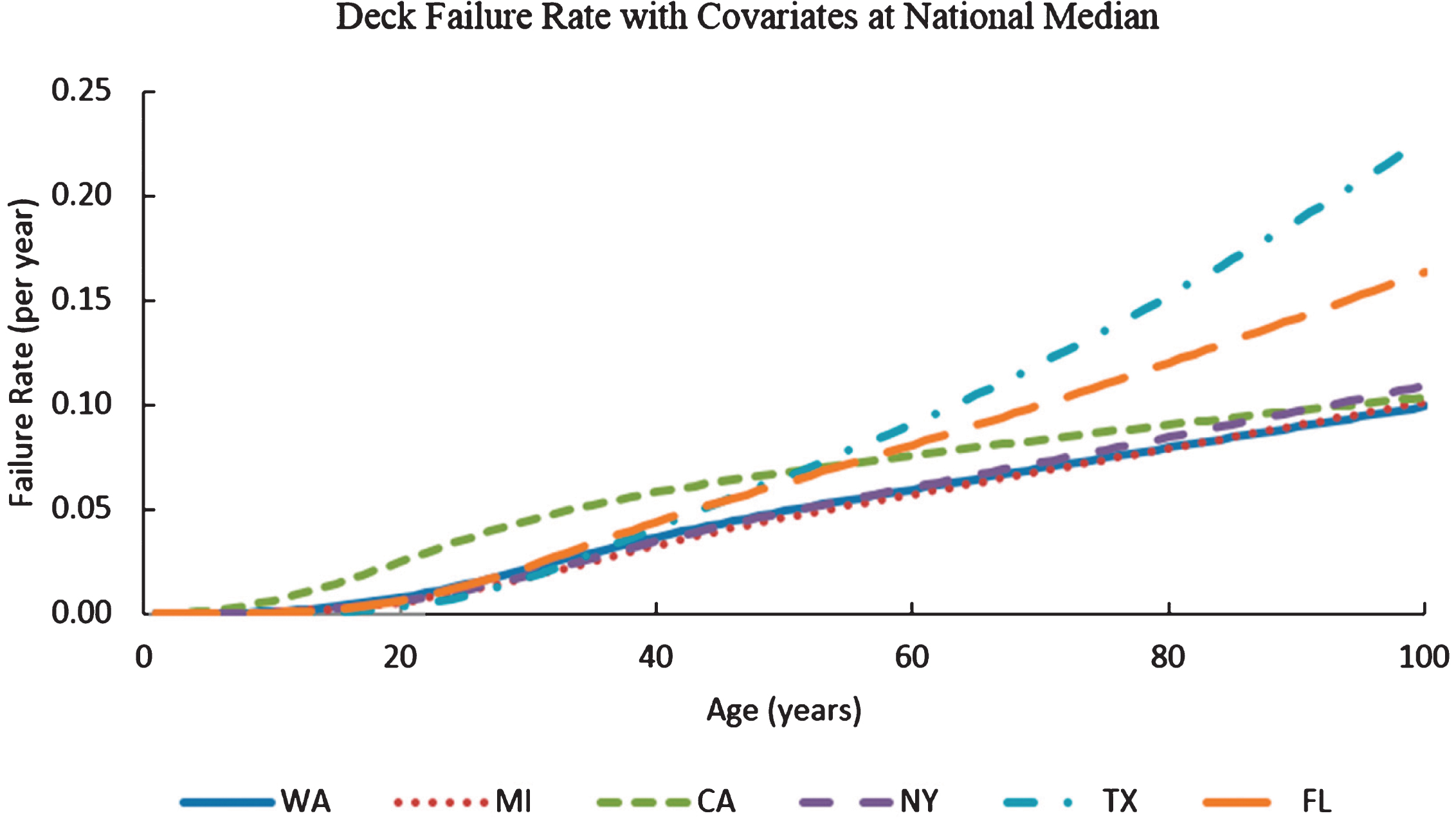
Fig.4
Variation of deck probability density function (PDF) with age for Washington State, California, Michigan, Florida, Texas, and New York with ADT and deck areas at national median (ADT = 1703 and deck area = 355.3 m2).
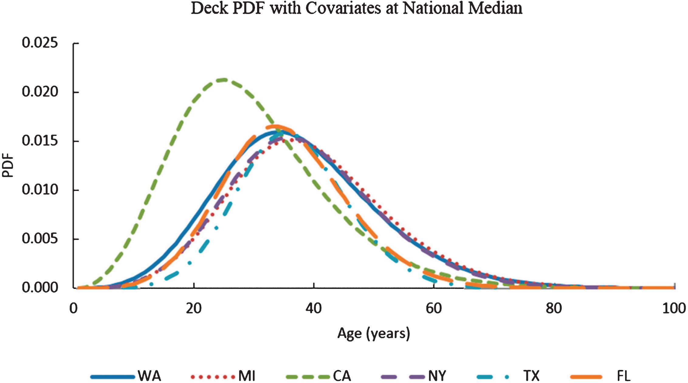
Table 1
Median and mean values of ADT and deck area for each state
| State | ADT | Deck area | ||
| Mean | Median | Mean (m2) | Median (m2) | |
| Alaska | 3489 | 800 | 755.0 | 382.2 |
| Alabama | 6446 | 1500 | 942.7 | 502.1 |
| Arkansas | 4635 | 1300 | 744.6 | 365.8 |
| Arizona | 17505 | 6400 | 1191.4 | 605.6 |
| California | 28358 | 8000 | 1165.2 | 556.8 |
| Colorado | 11608 | 4000 | 759.3 | 431.3 |
| Connecticut | 23398 | 10900 | 912.8 | 546.6 |
| Delaware | 15594 | 11206 | 1105.4 | 547.5 |
| Florida | 20579 | 10436 | 1459.7 | 663.0 |
| Georgia | 12474 | 2330 | 905.7 | 531.2 |
| Hawaii | 26911 | 11010 | 1156.9 | 277.0 |
| Iowa | 1602 | 130 | 357.3 | 198.9 |
| Idaho | 4227 | 570 | 451.8 | 192.4 |
| Illinois | 5355 | 350 | 499.2 | 220.0 |
| Indiana | 5472 | 506 | 414.6 | 200.1 |
| Kansas | 2498 | 88 | 501.0 | 301.8 |
| Kentucky | 5293 | 570.5 | 464.0 | 193.4 |
| Louisiana | 6864 | 1770 | 1425.0 | 336.6 |
| Massachusetts | 24167 | 12000 | 670.4 | 358.4 |
| Maryland | 29186 | 11270 | 1110.5 | 577.9 |
| Maine | 4757 | 2120 | 499.5 | 265.5 |
| Michigan | 9932 | 3300 | 584.0 | 342.4 |
| Minnesota | 7400 | 1360 | 788.8 | 468.8 |
| Missouri | 3742 | 114 | 473.7 | 191.5 |
| Mississippi | 4443 | 1641 | 923.1 | 543.5 |
| Montana | 4000 | 1880 | 627.0 | 436.2 |
| North Carolina | 8499 | 3700 | 810.3 | 506.2 |
| North Dakota | 2221 | 182.5 | 516.6 | 314.5 |
| Nebraska | 2014 | 75 | 377.1 | 168.4 |
| New Hampshire | 7136 | 2300 | 403.1 | 179.7 |
| New Jersey | 26327 | 13225 | 958.7 | 452.5 |
| New Mexico | 8300 | 3079 | 773.3 | 550.5 |
| Nevada | 21735 | 6950 | 1274.7 | 752.2 |
| New York | 13472 | 4476.5 | 823.6 | 448.0 |
| Ohio | 8306 | 1570 | 557.8 | 267.2 |
| Oklahoma | 3099 | 100 | 469.7 | 197.5 |
| Oregon | 9086 | 2600 | 809.5 | 417.1 |
| Pennsylvania | 7174 | 2830 | 605.0 | 245.8 |
| Puerto Rico | 18485 | 8100 | 941.4 | 357.5 |
| Rhode Island | 21217 | 12700 | 799.5 | 479.5 |
| South Carolina | 4257 | 780 | 699.3 | 267.2 |
| South Dakota | 1478 | 139.5 | 390.5 | 264.8 |
| Tennessee | 11783 | 2030 | 787.7 | 435.5 |
| Texas | 11641 | 3600 | 1167.0 | 570.8 |
| Utah | 15911 | 4587 | 793.4 | 493.7 |
| Virginia | 11225 | 3552 | 899.8 | 474.4 |
| Vermont | 2729 | 985 | 320.5 | 151.2 |
| Washington | 12316 | 4098 | 962.8 | 460.5 |
| Wisconsin | 6050 | 980 | 489.5 | 226.3 |
| West Virginia | 7068 | 3075 | 875.9 | 461.3 |
| Wyoming | 2696 | 1841 | 490.3 | 353.8 |
| USA (overall) | 9687 | 1703 | 755.9 | 355.3 |
Table 2
Median, mean, and standard deviation for age of bridges with a deck rating of 5 in each state
| State | No.of bridges | Age | ||
| Mean (years) | Median (years) | Standard deviation (years) | ||
| Alaska | 45 | 44.6 | 44.0 | 12.9 |
| Alabama | 953 | 57.9 | 56.0 | 14.3 |
| Arkansas | 357 | 52.2 | 48.0 | 14.3 |
| Arizona | 279 | 46.3 | 43.0 | 17.8 |
| California | 2509 | 39.3 | 40.0 | 16.4 |
| Colorado | 292 | 52.2 | 48.0 | 14.7 |
| Connecticut | 145 | 54.3 | 52.0 | 14.6 |
| Delaware | 30 | 47.8 | 47.5 | 11.7 |
| Florida | 128 | 47.9 | 47.0 | 15.1 |
| Georgia | 644 | 53.3 | 51.5 | 13.4 |
| Hawaii | 141 | 63.2 | 62.0 | 21.9 |
| Iowa | 2120 | 56.7 | 52.0 | 18.3 |
| Idaho | 162 | 50.2 | 46.0 | 15.1 |
| Illinois | 1046 | 54.9 | 48.0 | 22.9 |
| Indiana | 1105 | 49.9 | 45.0 | 21.1 |
| Kansas | 971 | 69.0 | 74.0 | 17.8 |
| Kentucky | 989 | 53.0 | 50.0 | 17.9 |
| Louisiana | 250 | 48.1 | 46.0 | 11.9 |
| Massachusetts | 598 | 55.4 | 51.0 | 15.4 |
| Maryland | 288 | 58.0 | 51.0 | 19.3 |
| Maine | 201 | 62.5 | 61.0 | 17.0 |
| Michigan | 779 | 54.6 | 51.0 | 18.7 |
| Minnesota | 507 | 58.6 | 51.0 | 20.9 |
| Missouri | 1323 | 65.5 | 64.0 | 20.9 |
| Mississippi | 423 | 52.4 | 51.0 | 18.0 |
| Montana | 186 | 44.7 | 44.0 | 15.5 |
| North Carolina | 1068 | 48.7 | 48.0 | 15.0 |
| North Dakota | 106 | 60.5 | 60.0 | 14.1 |
| Nebraska | 1539 | 42.7 | 38.0 | 22.6 |
| New Hampshire | 122 | 62.4 | 65.5 | 17.4 |
| New Jersey | 584 | 56.9 | 53.0 | 18.6 |
| New Mexico | 166 | 45.6 | 42.0 | 14.6 |
| Nevada | 23 | 42.7 | 39.0 | 15.4 |
| New York | 1288 | 53.9 | 50.0 | 17.7 |
| Ohio | 1085 | 54.9 | 50.0 | 19.7 |
| Oklahoma | 1609 | 57.5 | 61.0 | 19.4 |
| Oregon | 331 | 50.4 | 49.0 | 17.2 |
| Pennsylvania | 2045 | 62.5 | 63.0 | 19.0 |
| Puerto Rico | 498 | 44.8 | 39.0 | 20.1 |
| Rhode Island | 58 | 50.3 | 45.0 | 17.2 |
| South Carolina | 892 | 47.8 | 49.0 | 14.1 |
| South Dakota | 552 | 56.3 | 54.0 | 19.4 |
| Tennessee | 976 | 50.1 | 49.5 | 16.6 |
| Texas | 672 | 49.9 | 48.0 | 13.8 |
| Utah | 135 | 44.2 | 43.0 | 14.1 |
| Virginia | 1060 | 54.1 | 50.0 | 17.3 |
| Vermont | 139 | 65.2 | 69.0 | 16.5 |
| Washington | 145 | 51.5 | 49.0 | 18.1 |
| Wisconsin | 941 | 50.7 | 47.0 | 19.5 |
| West Virginia | 389 | 57.9 | 60.0 | 21.6 |
| Wyoming | 436 | 37.9 | 39.0 | 12.3 |
| USA (overall) | 33320 | 53.2 | 50.0 | 19.5 |
Table 3
Best-fit parameters for each state to be used in reliability and failure rate equations
| State | Best-fit parameters | |||
| α | β | c | d | |
| Alaska | 2.40012E-04 | 2.48068E+00 | 1.24052E-04 | −8.71859E-06 |
| Alabama | 1.10356E-05 | 3.12302E+00 | 1.84790E-06 | 9.96658E-06 |
| Arkansas | 1.10151E-04 | 2.61217E+00 | 5.75697E-06 | 3.66707E-06 |
| Arizona | 7.25463E-04 | 2.09590E+00 | 7.89339E-05 | 8.30138E-06 |
| California | 6.12317E-03 | 1.61358E+00 | 3.16064E-06 | −7.12924E-08 |
| Colorado | 6.03398E-05 | 2.72481E+00 | 1.19852E-04 | 3.08240E-06 |
| Connecticut | 1.28433E-05 | 3.10522E+00 | 1.62743E-04 | 4.68624E-07 |
| Delaware | 3.18833E-05 | 3.01570E+00 | 2.00883E-05 | 4.66263E-07 |
| Florida | 2.70608E-04 | 2.38221E+00 | 1.21644E-05 | 6.80383E-06 |
| Georgia | 4.11230E-05 | 2.85738E+00 | 2.50970E-05 | 2.90705E-06 |
| Hawaii | 4.00186E-05 | 2.65459E+00 | 6.64110E-07 | 4.60596E-06 |
| Iowa | 2.47988E-04 | 2.32145E+00 | 9.33048E-05 | 1.10562E-05 |
| Idaho | 1.04694E-04 | 2.59679E+00 | 1.58452E-04 | 4.56839E-06 |
| Illinois | 1.97466E-03 | 1.76608E+00 | 8.42506E-05 | 3.24109E-06 |
| Indiana | 2.65098E-03 | 1.71996E+00 | 2.58603E-04 | 7.41835E-06 |
| Kansas | 9.56513E-06 | 3.01874E+00 | 2.44030E-04 | 5.93978E-05 |
| Kentucky | 6.18934E-04 | 2.11412E+00 | 6.21635E-05 | 2.37579E-06 |
| Louisiana | 5.61499E-05 | 2.89531E+00 | −1.27973E-05 | −2.94284E-06 |
| Massachusetts | 4.03333E-05 | 2.79115E+00 | 4.90888E-05 | 1.98957E-06 |
| Maryland | 1.55452E-04 | 2.39922E+00 | 7.33951E-05 | 2.86109E-06 |
| Maine | 6.65890E-06 | 3.13124E+00 | 4.06957E-04 | 4.20086E-06 |
| Michigan | 5.37853E-04 | 2.12073E+00 | 8.75032E-05 | 2.93410E-06 |
| Minnesota | 6.88674E-04 | 2.02791E+00 | 7.73901E-05 | 1.67141E-06 |
| Missouri | 1.84442E-04 | 2.31123E+00 | 6.81506E-05 | 8.23692E-06 |
| Mississippi | 3.38631E-04 | 2.22499E+00 | 1.23919E-04 | 7.30707E-06 |
| Montana | 7.80047E-04 | 2.10365E+00 | 7.60406E-05 | 1.00547E-05 |
| North Carolina | 1.51371E-04 | 2.52035E+00 | 4.83642E-05 | 6.32536E-06 |
| North Dakota | 3.62227E-07 | 3.90483E+00 | 6.02702E-04 | 2.53707E-05 |
| Nebraska | 1.92160E-02 | 1.20339E+00 | 2.99383E-04 | −1.75632E-05 |
| New Hampshire | 2.35083E-05 | 2.85464E+00 | 2.69781E-04 | 6.84654E-07 |
| New Jersey | 4.83632E-04 | 2.15250E+00 | 2.37113E-05 | 8.18356E-08 |
| New Mexico | 3.05700E-04 | 2.35681E+00 | 1.11534E-04 | 1.14321E-05 |
| Nevada | 1.15542E-03 | 2.06775E+00 | −1.26181E-05 | 1.97310E-06 |
| New York | 5.21923E-04 | 2.15703E+00 | 1.01723E-05 | 1.75436E-06 |
| Ohio | 6.52566E-04 | 2.07661E+00 | 1.68105E-05 | 4.30575E-06 |
| Oklahoma | 3.89457E-04 | 2.17592E+00 | 8.64024E-05 | 8.86447E-06 |
| Oregon | 8.35826E-04 | 2.05258E+00 | 5.72566E-06 | 2.32944E-06 |
| Pennsylvania | 1.64122E-04 | 2.36994E+00 | 2.32485E-05 | 5.99993E-06 |
| Puerto Rico | 3.37961E-03 | 1.68367E+00 | 4.70402E-05 | 3.97620E-06 |
| Rhode Island | 1.76890E-04 | 2.43201E+00 | 1.33248E-04 | 1.18117E-06 |
| South Carolina | 3.17635E-04 | 2.38018E+00 | 2.56668E-05 | −7.23739E-08 |
| South Dakota | 5.50121E-04 | 2.10123E+00 | 5.00583E-05 | 3.60474E-05 |
| Tennessee | 4.44086E-04 | 2.21970E+00 | 6.53395E-05 | 3.51441E-06 |
| Texas | 5.70019E-05 | 2.79476E+00 | 5.04933E-06 | 4.10666E-06 |
| Utah | 3.60046E-04 | 2.36062E+00 | 7.18710E-05 | 1.08483E-06 |
| Virginia | 3.32972E-04 | 2.26964E+00 | 2.39130E-05 | 2.61294E-06 |
| Vermont | 5.88618E-07 | 3.66054E+00 | 3.96879E-04 | 1.46214E-05 |
| Washington | 9.94355E-04 | 1.99624E+00 | 2.92980E-07 | 3.88517E-06 |
| Wisconsin | 1.20264E-03 | 1.93514E+00 | 8.59890E-05 | 8.20458E-06 |
| West Virginia | 2.62431E-04 | 2.24105E+00 | 6.34800E-05 | 1.22325E-05 |
| Wyoming | 1.07624E-03 | 2.14952E+00 | 1.45998E-04 | −1.02956E-05 |
Table 4
Reliability and failure rates at age 50 with covariates at national or states’ medians
| State | Reliability and failure rates at age 50 ADT and deck area at: | |||
| State’s median | National median | |||
| Reliability | Failure rate (per year) | Reliability | Failure rate (per year) | |
| Alaska | 0.336 | 0.087 | 0.352 | 0.085 |
| Alabama | 0.772 | 0.046 | 0.770 | 0.046 |
| Arkansas | 0.563 | 0.061 | 0.561 | 0.061 |
| Arizona | 0.404 | 0.065 | 0.475 | 0.057 |
| California | 0.244 | 0.067 | 0.244 | 0.067 |
| Colorado | 0.588 | 0.061 | 0.612 | 0.058 |
| Connecticut | 0.626 | 0.065 | 0.680 | 0.058 |
| Delaware | 0.435 | 0.089 | 0.449 | 0.087 |
| Florida | 0.414 | 0.073 | 0.501 | 0.062 |
| Georgia | 0.604 | 0.062 | 0.613 | 0.061 |
| Hawaii | 0.861 | 0.027 | 0.887 | 0.023 |
| Iowa | 0.656 | 0.045 | 0.619 | 0.048 |
| Idaho | 0.583 | 0.059 | 0.539 | 0.064 |
| Illinois | 0.572 | 0.040 | 0.557 | 0.041 |
| Indiana | 0.459 | 0.048 | 0.410 | 0.053 |
| Kansas | 0.870 | 0.030 | 0.772 | 0.044 |
| Kentucky | 0.563 | 0.049 | 0.549 | 0.050 |
| Louisiana | 0.384 | 0.092 | 0.384 | 0.092 |
| Massachusetts | 0.700 | 0.049 | 0.725 | 0.046 |
| Maryland | 0.686 | 0.043 | 0.732 | 0.038 |
| Maine | 0.825 | 0.039 | 0.790 | 0.044 |
| Michigan | 0.597 | 0.046 | 0.601 | 0.046 |
| Minnesota | 0.637 | 0.040 | 0.645 | 0.039 |
| Missouri | 0.799 | 0.030 | 0.779 | 0.032 |
| Mississippi | 0.602 | 0.048 | 0.628 | 0.045 |
| Montana | 0.406 | 0.065 | 0.416 | 0.064 |
| North Carolina | 0.509 | 0.065 | 0.537 | 0.062 |
| North Dakota | 0.721 | 0.066 | 0.603 | 0.085 |
| Nebraska | 0.305 | 0.044 | 0.287 | 0.046 |
| New Hampshire | 0.810 | 0.037 | 0.763 | 0.043 |
| New Jersey | 0.626 | 0.044 | 0.629 | 0.044 |
| New Mexico | 0.372 | 0.077 | 0.423 | 0.071 |
| Nevada | 0.311 | 0.076 | 0.317 | 0.075 |
| New York | 0.577 | 0.049 | 0.583 | 0.048 |
| Ohio | 0.607 | 0.044 | 0.605 | 0.044 |
| Oklahoma | 0.685 | 0.039 | 0.656 | 0.042 |
| Oregon | 0.520 | 0.052 | 0.523 | 0.051 |
| Pennsylvania | 0.759 | 0.035 | 0.763 | 0.035 |
| Puerto Rico | 0.396 | 0.053 | 0.421 | 0.050 |
| Rhode Island | 0.555 | 0.058 | 0.594 | 0.054 |
| South Carolina | 0.425 | 0.071 | 0.422 | 0.072 |
| South Dakota | 0.643 | 0.041 | 0.576 | 0.048 |
| Tennessee | 0.517 | 0.056 | 0.525 | 0.056 |
| Texas | 0.552 | 0.067 | 0.566 | 0.065 |
| Utah | 0.347 | 0.081 | 0.365 | 0.079 |
| Virginia | 0.598 | 0.049 | 0.607 | 0.049 |
| Vermont | 0.942 | 0.022 | 0.891 | 0.034 |
| Washington | 0.522 | 0.050 | 0.533 | 0.049 |
| Wisconsin | 0.521 | 0.048 | 0.502 | 0.050 |
| West Virginia | 0.711 | 0.038 | 0.734 | 0.035 |
| Wyoming | 0.178 | 0.104 | 0.177 | 0.104 |
Table 5
Calculated p-values associated with deck area and ADT in different states
| State | p value | State | p value | ||
| Deck Area | ADT | Deck Area | ADT | ||
| Alaska | 0.272 | 0.292 | North Carolina | 1.54 × 10⁻³¹ | 3.19 × 10⁻²³ |
| Alabama | 0.212 | 8.65 × 10–43 | North Dakota | 3.55 × 10⁻⁷ | 0.283 |
| Arkansas | 0.173 | 0.011 | Nebraska | 3.05 × 10⁻⁵ | 0.050 |
| Arizona | 7.18 × 10⁻⁶ | 6.03 × 10⁻⁹ | New Hampshire | 5.21 × 10⁻⁷ | 0.172 |
| California | 0.012 | 0.335 | New Jersey | 3.42 × 10⁻⁴ | 0.137 |
| Colorado | 1.90 × 10⁻⁸ | 1.36 × 10⁻³ | New Mexico | 0.021 | 1.33 × 10⁻³ |
| Connecticut | 3.13 × 10⁻¹⁶ | 0.493 | Nevada | 0.321 | 0.371 |
| Delaware | 0.173 | 0.132 | New York | 4.29 × 10⁻⁵ | 1.14 × 10⁻⁶ |
| Florida | 0.446 | 1.88 × 10⁻⁴ | Ohio | 1.10 × 10⁻³ | 1.50 × 10⁻¹² |
| Georgia | 5.55 × 10⁻³ | 4.21 × 10⁻⁴ | Oklahoma | 5.46 × 10⁻²⁹ | 6.71 × 10⁻¹⁹ |
| Hawaii | 0.215 | 5.01 × 10⁻²² | Oregon | 0.092 | 0.013 |
| Iowa | 3.39 × 10⁻²⁸ | 3.80 × 10⁻¹⁰ | Pennsylvania | 1.39 × 10⁻¹⁶ | 4.46 × 10⁻²⁵ |
| Idaho | 3.81 × 10⁻⁵ | 5.58 × 10⁻³ | Puerto Rico | 5.15 × 10⁻¹⁰ | 2.25 × 10⁻⁹ |
| Illinois | 2.04 × 10⁻²¹ | 1.43 × 10⁻⁴ | Rhode Island | 1.55 × 10⁻⁶ | 0.383 |
| Indiana | 1.42 × 10⁻³⁵ | 2.59 × 10⁻³ | South Carolina | 6.47 × 10⁻⁵ | 0.039 |
| Kansas | 6.56 × 10–43 | 1.12 × 10⁻¹¹ | South Dakota | 6.71 × 10⁻⁴ | 2.80 × 10⁻¹⁰ |
| Kentucky | 7.28 × 10⁻⁹ | 1.53 × 10⁻³ | Tennessee | 1.19 × 10⁻¹⁵ | 1.56 × 10⁻⁹ |
| Louisiana | 0.135 | 0.063 | Texas | 0.016 | 4.71 × 10⁻²¹ |
| Massachusetts | 7.51 × 10⁻⁹ | 5.16 × 10⁻¹² | Utah | 3.00 × 10⁻³ | 0.446 |
| Maryland | 6.55 × 10⁻¹⁴ | 3.46 × 10⁻¹⁰ | Virginia | 1.19 × 10⁻⁹ | 1.24 × 10⁻⁸ |
| Maine | 5.17 × 10⁻²⁰ | 0.273 | Vermont | 6.71 × 10⁻¹⁹ | 1.87 × 10⁻³ |
| Michigan | 3.53 × 10⁻¹⁰ | 2.92 × 10⁻⁴ | Washington | 0.015 | 0.099 |
| Minnesota | 1.20 × 10⁻⁸ | 0.157 | Wisconsin | 2.95 × 10⁻¹⁶ | 5.16 × 10⁻¹⁰ |
| Missouri | 2.29 × 10⁻²² | 6.80 × 10⁻¹⁷ | West Virginia | 5.39 × 10⁻⁹ | 1.23 × 10⁻¹⁵ |
| Mississippi | 1.37 × 10⁻⁸ | 2.68 × 10⁻⁷ | Wyoming | 4.22 × 10⁻⁶ | 0.093 |
| Montana | 5.40 × 10⁻³ | 0.030 | |||


