Argumentative explanations for pattern-based text classifiers

Lertvittayakumjorn, Piyawat; Toni, Francesca

doi:10.3233/AAC-220004

Argumentative explanations for pattern-based text classifiers

Article type: Research Article

Authors: Lertvittayakumjorn, Piyawat^{; *} | Toni, Francesca

Affiliations: Department of Computing, Imperial College London, United Kingdom

Correspondence: [*] Corresponding author. E-mail: [email protected].

Keywords: Explainable AI, argumentative explanation, logistic regression, text classification

DOI: 10.3233/AAC-220004

Journal: Argument & Computation, vol. 14, no. 2, pp. 163-234, 2023

Published: 7 June 2023

Get PDF

Abstract

Recent works in Explainable AI mostly address the transparency issue of black-box models or create explanations for any kind of models (i.e., they are model-agnostic), while leaving explanations of interpretable models largely underexplored. In this paper, we fill this gap by focusing on explanations for a specific interpretable model, namely pattern-based logistic regression (PLR) for binary text classification. We do so because, albeit interpretable, PLR is challenging when it comes to explanations. In particular, we found that a standard way to extract explanations from this model does not consider relations among the features, making the explanations hardly plausible to humans. Hence, we propose AXPLR, a novel explanation method using (forms of) computational argumentation to generate explanations (for outputs computed by PLR) which unearth model agreements and disagreements among the features. Specifically, we use computational argumentation as follows: we see features (patterns) in PLR as arguments in a form of quantified bipolar argumentation frameworks (QBAFs) and extract attacks and supports between arguments based on specificity of the arguments; we understand logistic regression as a gradual semantics for these QBAFs, used to determine the arguments’ dialectic strength; and we study standard properties of gradual semantics for QBAFs in the context of our argumentative re-interpretation of PLR, sanctioning its suitability for explanatory purposes. We then show how to extract intuitive explanations (for outputs computed by PLR) from the constructed QBAFs. Finally, we conduct an empirical evaluation and two experiments in the context of human-AI collaboration to demonstrate the advantages of our resulting AXPLR method.

1.Introduction

Humans have been using explanations in AI for many purposes such as to support human decision making [35,39], to increase human trust in the AI [27,65], to verify and improve the AI [10,40], and to learn new knowledge from the AI [34,44]. Explanations may also be required for an AI-assisted system to comply with recent regulations including the General Data Protection Regulation (GDPR) [21]. These various needs for explanation have drawn a great amount of attention to the field of explainable AI (XAI) in recent years [1]. When an AI-assisted system is used for prediction (referred to as a prediction model or simply a model in the literature and in this paper), explanations for the system behavior are often categorized broadly into two types: local explanations and global explanations [1], where the former focus on explaining the predictions for specific inputs while the latter aim to explain the behavior of the model in general, irrespective of any inputs that it may take. If the model is inherently interpretable [58] (e.g., a decision tree), the model itself can be viewed as the global explanation whereas local explanations can be obtained during the prediction process (e.g., the corresponding path in the decision tree for the input, leading to the output/prediction). In this paper, we refer to explanations straightforwardly extracted from inherently interpretable models (e.g., the applicable path in a decision tree) as model-inherent explanations. However, if the model is opaque (e.g., it is a deep learning model), we may need to apply an additional step, by using a so-called post-hoc explanation method (e.g., LIME [54] and SHAP [43]), for extracting the explanations.

A number of properties of explanations have been identified as desirable in the literature, e.g., as in [62]. Amongst them, generally, we call an explanation faithful to the model if it accurately reflects the true reasoning process of the model, whereas an explanation is deemed plausible if it agrees with human judgement (e.g., as discussed in [26]). These two properties of explanations, i.e., faithfulness and plausibility, may be important in different situations. For instance, we want faithful explanations in order to verify the model correctness while we want plausible explanations to satisfy end users. Note that model-inherent explanations can be deemed faithful due to their straightforward and sensible explanation extraction process. However, this does not guarantee other desirable properties of the explanations. For instance, using a decision tree path with depth of 15 as an explanation is not comprehensible to humans and, therefore, not very plausible either. Post-hoc explanations could be more effective for impressing end-users in this case though they are not inherently extracted from (or perfectly faithful to) the underlying interpretable model (i.e., the decision tree).

In this paper, we develop a novel post-hoc local explanation method that aims to generate plausible explanations for a specific class of interpretable prediction models performing binary text classification with natural language data. Binary text classification aims to classify a given text into one of two possible categories. Examples of binary text classification (both studied in this paper) are sentiment analysis (where a piece of text is classified as having positive or negative sentiment) and spam detection (where a message is classified as spam or not). Our interpretable prediction models are built using logistic regression (LR) [29, chapter 5] with textual patterns [60] as features. LR is a traditional machine learning method, leading to interpretable models with linear combinations of features, that can be used, in particular, for text classification [29, chapter 5]. Because text documents are unstructured data, we need to perform feature extraction so as to obtain numerical representations of the documents before training the LR classifier. One standard way to do feature extraction is using frequent n-grams (i.e., frequent n consecutive words in the dataset) as features and applying TF-IDF vectorization to find associated values of the features [71, chapter 2]. Though using n-grams as features is simple and often effective, it makes the model less generalizable to words or n-grams that have never appeared during training. Also, the features are usually too fine-grained for humans to synthesize the overview of what the model has learned even though LR is inherently interpretable. In this paper, as elsewhere (e.g., [9,20,25]), we use patterns as features for prediction, in alternative to n-gram features. Specifically, we exploit the interpretability of the patterns, as in [18], but by using them as features for logistic regression models. We call our models of interest pattern-based logistic regression (PLR) models.1 1

PLR models are inherently interpretable because LR is interpretable and because their features are interpretable and, as we will show, convenient for humans to learn or to extract knowledge from. However, their model-inherent explanations for PLR may not be plausible. This issue is especially critical when interactions among input features underpin the model whereas the model-inherent explanations treat features independently of each other. These feature interactions may result from agreement or disagreement between correlated pattern features. In order to address this problem, our proposed explanation method leverages computational argumentation (CA) to take care of the feature interactions and generate more plausible local explanations than the model-inherent explanations. We call our novel explanation method (applying CA to better explain PLR) Argumentative eXplanations for Pattern-based Logistic Regression (AXPLR, pronounced “ax-plore”).2 2

Generally, local explanations often have an argumentative spirit by nature since they need to argue for or against possible predictions of the model [14]. When there are several arguments involved, these arguments may also have dialectical relationships between each other. Hence, there are several existing works which use computational argumentation to underpin XAI methods and produce argumentative explanations. For example, DEAr [12] considers related training examples as arguments, which argue to classify a test example, and uses a dispute tree [15] as dialectical explanation. DAX [16] extracts local argumentative explanations from a deep neural network by using arguments and their relations to represent the nodes and their connections in the neural network. (For more approaches, see recent survey papers of argumentative XAI [14,67].) In our work, AXPLR uses pattern-based input features of the PLR model as arguments and draws dialectical relations from specificity of the pattern features. All are modeled using modified versions of Quantitative Bipolar Argumentation Frameworks (QBAFs) [7] before being processed and translated into argumentative explanations for human consumption. Specifically, we use two variants of QBAFs. Both include a mapping associating arguments with the classification they advocate, in addition to arguments, attack and support relations and base scores as in standard QBAFs. The two variants differ in the way they use specificity of patterns to define the direction of attacks and supports.

We summarize the contribution of our work as follows.

We show that model-inherent local explanations for pattern-based logistic regression can lead to implausible explanations.
We propose AXPLR, a novel argumentative explanation method, to tackle the above problem by modeling relationships among pattern features using quantitative bipolar argumentation.
We prove that the argumentation framework underpinning AXPLR always predicts the same output as the original PLR model and satisfies several dialectical properties of human debates.
Using three binary text classification datasets, we conduct an empirical evaluation of the extracted argumentation frameworks. Moreover, for the same datasets, we conduct two human experiments to evaluate how plausible and helpful AXPLR is for human consumption compared to other explanation methods.

Note that, although patterns and LR are widely used in machine learning, and thus their combination in PLR cannot be deemed novel, we are the first, to the best of our knowledge, to show that PLR can be fruitfully used for NLP tasks to obtain explainable predictions. Furthermore, plausibility of the explanations could be improved using the CA-based explanation method proposed in this paper.

In the remainder of the paper, we explain the pattern-based logistic regression (PLR) model in Section 2. Then we discuss the weakness of the model-inherent explanations for PLR in Section 3. After that, Section 4 describes the two variants of QBAFs underpinning AXPLR, while Section 5 shows that these QBAFs satisfy many dialectical properties of human debates, leading to leaner derived AXPLR (of which the presentations are described in Section 6). Next, the experimental setup for AXPLR is explained in Section 7, followed by one empirical experiment in Section 8 and two human experiments (to assess the amenability of the argumentation underpinning AXPLR specifically) in Sections 9 and 10. Lastly, we discuss generalization and other possible uses of AXPLR in Section 11, position our work with respect to other related work in Section 12, and summarize the paper in Section 13. Code and datasets of this paper are available at https://github.com/plkumjorn/AXPLR.

2.Background

In this section, we provide necessary background on text classification (see Section 2.1) and PLR, including logistic regression (LR) which is the core machine learning method of PLR (see Section 2.2) and pattern features as well as the pattern extraction algorithm GrASP [60] used for constructing pattern features from training data (see Section 2.3). We conclude with an illustration of the overall process of PLR combining LR with GrASP for text classification (see Section 2.4). To illustrate ideas, we will use sentiment analysis as a running example of text classification throughout this section.

2.1.Binary text classification

We focus on the binary text classification task with two classes, using, as conventional, C={0,1} as the set of classes. For example, in the case of sentiment analysis, 0 stands for negative sentiment and 1 stands for positive sentiment. A training dataset D contains N different pairs of the form (x,y) where x is an input text and y∈C is the true class label of x. This dataset is used to train a classifier, which determines the probability of classes for any given input. In the context of binary text classification, D can be split into disjoint sets D+ and D−, containing positive examples (y=1) and negative examples (y=0) in D, respectively. A classifier trained on D determines, for input x, a class yˆ∈C.

2.2.Logistic regression

For each input text x, let us assume that x can be represented as a feature vector f=[f1,f2,…,fd] where fi is a feature and d⩾1 is the number of features used to represent x. Then, an LR model targeting binary classification gives

(1)P(y=1|x)=sigmoid(wTf+b)=sigmoid(∑i=1dwifi+b)=sigmoid(w1f1+w2f2+⋯+wdfd+b)

where w∈Rd and b∈R are weights and bias of the LR model, respectively. The sigmoid function (so called a logistic function) is used to convert any real number into a value between 0 and 1:

(2)sigmoid(z)=11+e−z

where z=0 yields sigmoid(z)=0.5. Note also that 1−sigmoid(z)=sigmoid(−z). Normally, if P(y=1|x)⩾0.5 (i.e., ∑i=1dwifi+b⩾0), we predict class 1 for input x (i.e., yˆ=1). Otherwise, we predict class 0 (i.e., yˆ=0).

The LR model is obtained after the training process is completed; it is fully characterized by w and b which minimize the objective function (typically the binary cross-entropy loss) to be used for predicting unseen examples (in some test datasets, for example).

The next questions are “How do the d features look like for text?” and “How can we obtain them?”. We use pattern features whereby patterns indicate high-level characteristics of words in input texts, in addition to specifying exact words or lemmas. These high-level characteristics include both syntactic attributes (such as part-of-speech tags) and semantic attributes (such as synonyms and hypernyms). Thereby, we choose GrASP for this purpose.

2.3.Pattern features and GrASP: GReedy augmented sequential patterns

GrASP is a supervised algorithm which learns expressive patterns able to distinguish two classes of text [60]. An example of GrASP pattern for distinguishing between positive and negative texts in sentiment analysis is

[[TEXT:nothing], [SENTIMENT:pos]] with two gaps allowed in-between.

This pattern matches, for example, a sequence of two words where the first word is “nothing” and the second word is a positive word according to a specific lexicon (such as the one released by [24]). Moreover, the pattern allows at most two additional words in-between to increase flexibility of the pattern. Examples of texts matched by this pattern include:

“There is nothing delicious in this dinner .” and

“... worse products . Nothing is delicate ! ...”

where the bold-face words are words matching components in the pattern.

GrASP is applied directly to the training data. In order to use it, we need to prepare two lists of texts containing positive and negative examples that we want to distinguish. Also, we need to specify some hyperparameters such as the desired number of patterns, the number of gaps allowed, the set of linguistic attributes which can appear in the patterns, and the maximum number of attributes per pattern. In the experiments in this paper, we employ the publicly released implementation of GrASP [38] which provides several built-in attributes that are suitable for classification tasks in general, e.g., the token text itself, its lemma, its hypernyms (according to wordnet [45]), part-of-speech tags, and sentiment tags. The resulting GrASP patterns are used as features in the LR model. Note, however, that we do not utilize the associated class GrASP assigns to each pattern to classify the input directly because GrASP does not tell us how to properly deal with the input that matches multiple (and potentially contradicting or relating) patterns. Instead, we use the patterns from GrASP only as features for training a classifier, letting the classifier decide how multiple patterns should play their roles and contribute to the final classification.

2.4.Pattern-based logistic regression using GrASP

Fig. 1.

Overview of the processes for training, using, and explaining PLR for binary text classification.

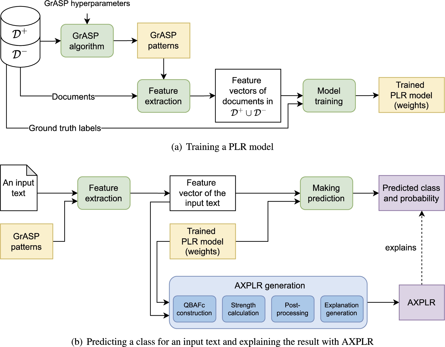
In this paper, we focus on PLR, i.e., LR with GrASP patterns as features. Figure 1(a) shows how to train such PLR model. First, we feed D+ and D− (as introduced in Section 2.1) to the GrASP algorithm along with some hyperparameters mentioned above. After obtaining the d GrASP patterns, we extract the binary feature vector f for each training example x and use it to train the LR model together with the ground truth class label y. Specifically, for each input text x∈D, we extract the feature vector f=[f1,f2,…,fd]∈{0,1}d where fi is a binary feature and d is the number of textual patterns used to represent x. fi equals 1 if the input x contains the pattern pi; otherwise, fi equals 0. Then, to learn from the training data D, we train a binary logistic regression model using the binary cross-entropy loss (with a regularization term) as objective function.

Next, Fig. 1(b) shows how to use the trained PLR model for prediction (and how our proposed explanation method AXPLR connects to the prediction process). Given an unseen input text x, we get the prediction by extracting the feature vector f using the d GrASP patterns and running the LR model on f. Figure 2 shows an illustrative example of how to make a prediction using a trained PLR model. Given the sentence “There is nothing better than hot sausages of this restaurant.” as an input text x, we want to use a trained PLR model to predict the sentiment of this sentence. Assume that among the d patterns of the model, there are only four patterns – p1, p2, p3, and p4 as shown in Fig. 2 – that match this sentence. In other words, for i∈{1,2,3,4}, fi=1; otherwise, fi=0. According to Equation (1), the probability of this text being a positive sentiment text, i.e., P(y=1|x), equals sigmoid(w1f1+w2f2+w3f3+w4f4+b). For the trained weights and bias in Fig. 2, the predicted class yˆ of x is positive (1) since the predicted probability is 0.5744, which is greater than 0.5.

3.Explaining pattern-based logistic regression classifiers: The need for argumentation

Since logistic regression is inherently interpretable and the GrASP patterns used are also interpretable, we can generate local explanations for inputs to a trained PLR model by reporting parts of the inputs that match the top-k patterns, in the spirit of much work in the XAI literature (e.g., [46, chapter 5] and [10]). Formally, given an input x, let si be the contribution of the pattern pi for the prediction yˆ, defined as follows, with reference to Equation (1): when yˆ=1, si=wifi; when yˆ=0, si=−wifi (so, we can combine both cases to be si=(−1)yˆ+1wifi). Then we can return, as the local explanation for yˆ, a list of triplets of the form (pi′,π(pi′,x),si′) where si′, the contribution of pattern pi′, is one of the k highest contributions and si′≠0, and π(pi′,x) is a part of x that matches the pattern pi′. We call this resulting model-inherent explanation the flat logistic regression explanation (FLX) (for x and yˆ). We adopt FLX as a baseline for PLR as it is the natural explanation method and commonly used with LR in general [8,53].

Fig. 2.

An illustrative example of using pattern-based logistic regression for sentiment analysis. (Here, FLX stands for flat logistic regression explanation, see Section 3.)

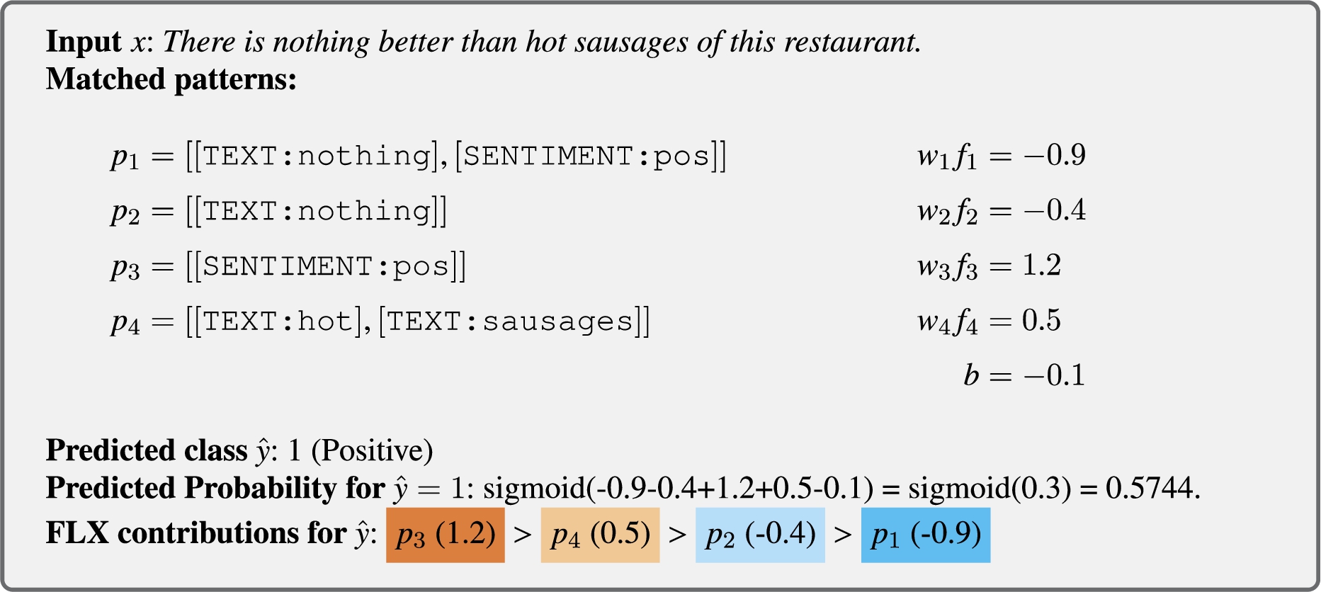
For the example in Fig. 2, the input text x matches four patterns, and the model predicts class positive (i.e., yˆ=1). If we use FLXs, we can see that p3 (which means the input text containing a positive word) has the highest contribution of 1.2. So, we will obtain (p3,π(p3,x),s3)=([[SENTIMENT:pos]],“better”,1.2) as the top triplet in the FLX (i.e., the most important reason) for predicting yˆ=1. Nevertheless, one problem with FLXs is that they do not take into account relationships among the patterns. For the example in Fig. 2, the model has actually weakened the effect of p3 by p1 because the positive word in this case (“better”) follows the word “nothing” and the model no longer considers it strongly positive in the context. What really makes the model answer positively is rather p4, which is considered less important by the FLX. Although the contribution of p4 (0.5) is lower than that of p3, it is not overridden by other patterns. We could see that these four patterns are arguing to make the prediction, in that each pattern is an argument for or against the prediction. Some patterns have dialectical relations with one another (such as the disagreement between p1 and p3). Hence, to improve plausibility of the explanations and make them in line with the underpinning dialectical relations, we apply computational argumentation, as shown next in Section 4, to generate local explanations for this PLR model.

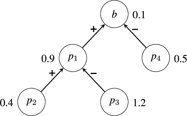
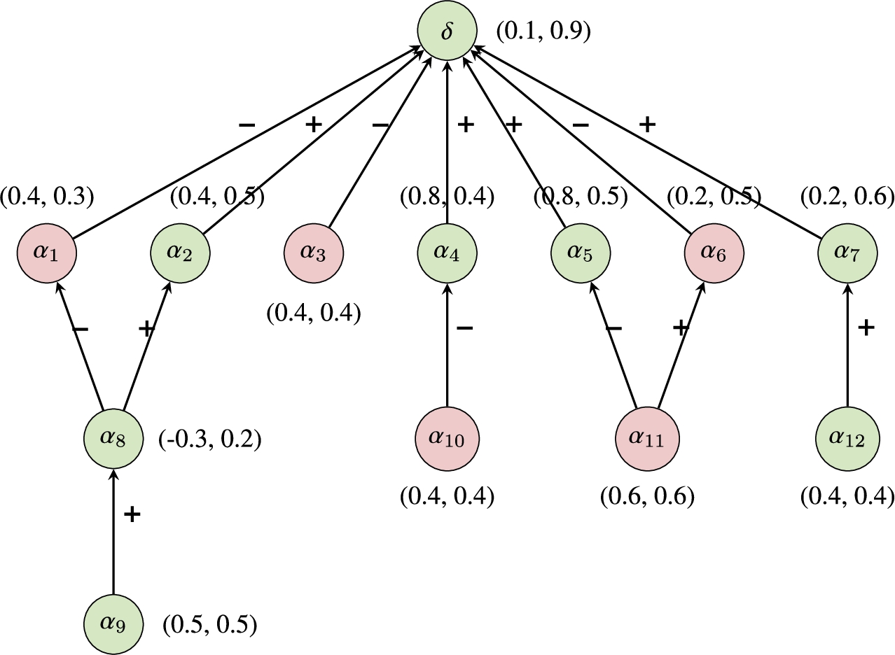
Fig. 3.

One possible QBAF. Arrows with plus and minus signs represent supports and attacks between arguments, respectively. The base score of each argument is displayed with a real number staying close to the argument.

Specifically, we aim to use a form of quantitative bipolar argumentation frameworks (QBAFs) [7] to simulate how the PLR model works on an input text. As background, a QBAF is a quadruple ⟨A,R−,R+,τ⟩, where A is a set of arguments, R− and R+ are binary relations of attack and support on A, respectively, and τ:A→I is a total function indicating the base score (internal strength) of each argument in A, staying in the range I (where, e.g., I is [0, 1], [−1, 1], [0, ∞)). This conceptualization of QBAF serves our purposes well, as, intuitively, (i) arguments in QBAFs can be used to represent applicable patterns and the model’s bias term, (ii) supports and attacks can reflect agreement and disagreement between these patterns, and (iii) base scores can represent the (learned) absolute weights of these patterns in the PLR model. Figure 3 displays one possible QBAF, for I=[0,∞) (we will see later that this QBAF can be read as capturing relations between patterns/the PLR’s bias term in Fig. 2). To show how each argument is affected by other arguments in a given QBAF, the argument’s dialectical strength can be computed (by using a strength function for aggregating the strengths of its attackers and the strengths of its supporters). Several notions of strength function exist in the literature (see e.g. [7] for an overview). We will use the dialectical strengths as a basis for generating plausible explanations for predictions, using a novel strength function matching the PLR model, to guarantee that the explanations are “equivalent” to the predictions being explained.

4.AXPLR: Argumentative explanations for pattern-based logistic regression

In this section, we introduce our AXPLR method, whose overall generation process is shown in Fig. 4, alongside the illustrative example from Fig. 2. In Fig. 4, the part above the purple line is the standard prediction process already captured in Fig. 2, starting from extracting the feature vector from the input text and then computing the predicted probability using the model weights (w and b). Below the purple line, Fig. 4 shows the four main steps for generating AXPLR. Using the feature vector and the model weights, the first step constructs a special type of quantitative bipolar argumentation framework (i.e., QBAFc) to represent relationships between the pattern features found in the input text. It contains arguments for patterns found in the input text as well as a default argument δ representing the bias term b of the PLR model. Note that the QBAFc after the first step in Fig. 4 corresponds to the QBAF in Fig. 3, but the QBAFc is special because each argument also supports a class in C, as represented by its background color. Particularly, the arguments with green background support the positive class, whereas the ones with red background support the negative class. The supported class, as well as the base score of the argument, is determined by the weight of the corresponding pattern (or the bias term b) in the PLR model.

Fig. 4.

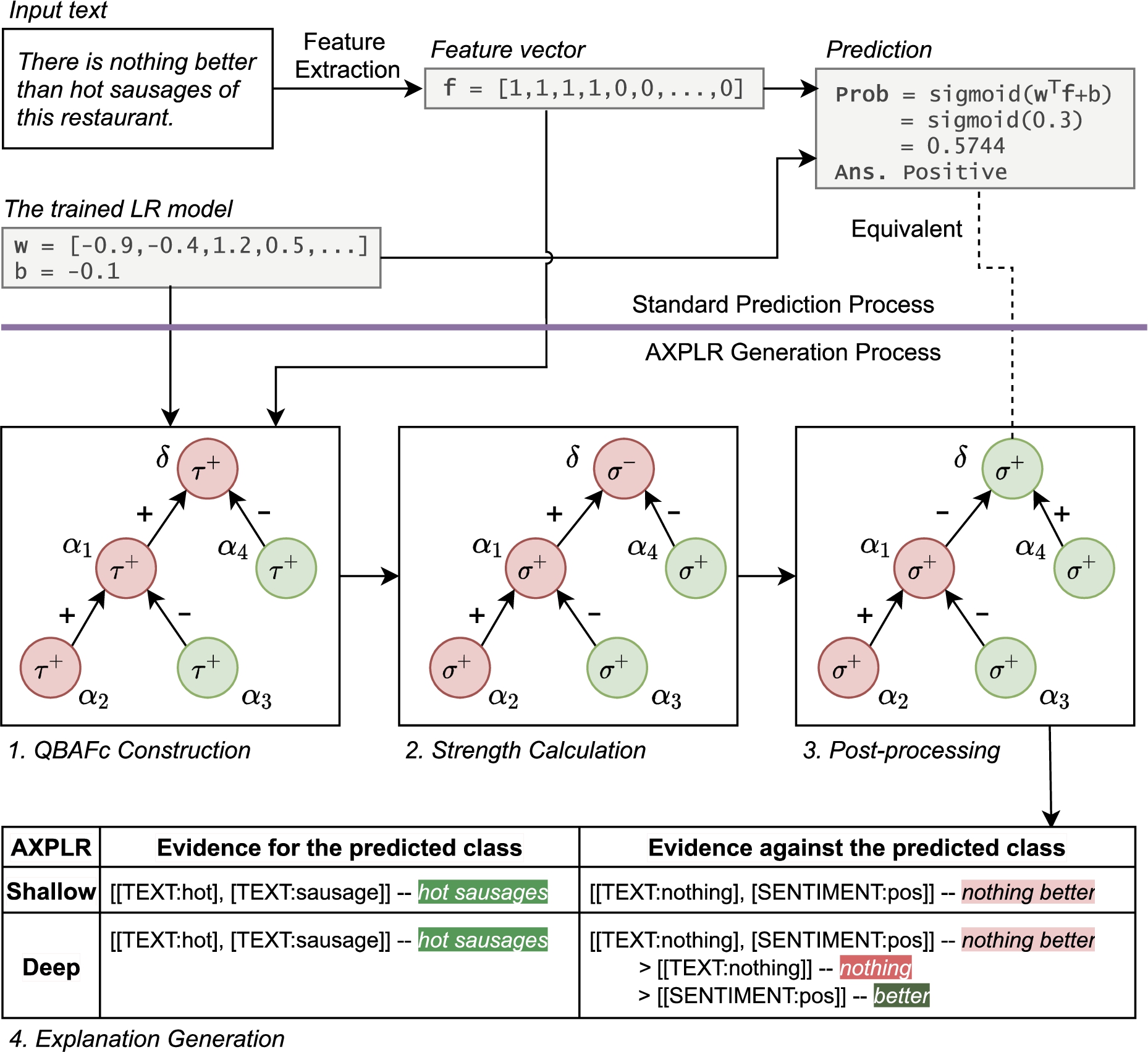
Overview of the AXPLR generation process. Above the purple line, it shows the standard prediction process of pattern-based logistic regression. Below the purple line, it shows the four main steps to generate AXPLR for the illustrative example from Fig. 2 (using a bottom-up QBAFc (BQBAFc), where edges labelled + indicate support and edges labelled − indicate attack). In step 1, τ+ indicates that all the base scores of the arguments are positive. In steps 2–3, σ+ and σ− indicate that the dialectical strengths of the arguments are positive and negative, respectively. In steps 1–3, the background color indicates the supported class (green indicates the positive class and red indicates the negative class). Step 4 automatically generates explanations from the QBAFc resulting from step 3. Particularly, we propose two kinds of explanations, i.e., shallow AXPLR (using only top-level arguments in the QBAFc to explain) or deep AXPLR (also using arguments at other levels in the QBAFc to explain). (See Section 4 for further details.)

The second step computes the dialectical strength of each argument, considering its attacker(s) and supporter(s). Here, we propose a new strength function, returning a real number score in (−∞,∞) that could reflect a class probability predicted by the PLR model (when the function is applied to the argument δ). With this new strength function, the dialectical strengths of some arguments might be negative, and thus possibly difficult to interpret (e.g., in Fig. 4, what does it mean for argument α1 (which supports the negative class) to support argument δ when the latter, having a negative strength, no longer supports the negative class?), so we do post-processing in the third step, making all the strength values to be positive and adjusting relations accordingly in a way that preserves the original meaning (e.g., in Fig. 4, after δ’s strength is flipped to be positive, its supported class then becomes the positive class; so, α1 needs to attack δ and α4 needs to support δ to preserve the original interactions between arguments). Finally, using the post-processed QBAFc, the fourth step generates the explanation which could be shallow (using only top-level arguments in the QBAFc) or deep (also using arguments at other levels in the QBAFc), as illustrated in the bottom table of Fig. 4. For each included argument αi, the explanation shows the corresponding pattern, the input text fragment matching the pattern, the post-processed argument strength (represented by the background color of the text fragments), and whether it is evidence for or against the predicted class. Before being presented to the users, this explanation table could be reorganized or embellished with descriptive texts to help users read the patterns and better appreciate the explanation (see Figs 9 and 10 for examples).

In the remainder of this section, we provide details for the first three steps of the AXPLR generation process (in Sections 4.1, 4.2, and 4.3, respectively). Then, in Section 6, we give details of step 4. Before that, in Section 5, we prove formal properties of (original and post-processed) QBAFcs, providing formal guarantees about their suitability to give rise to explanations.

4.1.QBAFc construction

To begin with, we define how two patterns can be related.

Definition 1.

A pattern p1 is more specific than or equivalent to another pattern p2 (written as p1⪰p2) if and only if for every text t matched by p1, t is also matched by p2. In addition, p1 is more specific than p2 (written as p1≻p2) if and only if p1⪰p2 but p2⋡p1.

For instance, we can say from Fig. 2 that p1⪰p3 because every text matched by p1 is guaranteed to have a positive sentiment word which makes it matched by p3. However, p3⋡p1 because a text matched by p3 is guaranteed to have a positive word but it may not have the word “nothing” followed by a positive word. These two facts also imply p1≻p3. Similarly, p1≻p2.

Lemma 1.

The relation ≻ is not reflexive and not symmetric, but it is transitive.

Proof.

See Appendix A.1. □

Next, we extract argumentation frameworks from a trained PLR model and a target input text x. These argumentation frameworks, like QBAFs [7], envisage that arguments can attack or support arguments, and that they are equipped with a base score. However, these frameworks differ from QBAFs in that the arguments therein support3 3 classes (as indicated by the signs of the corresponding parameters in the PLR model). Moreover, these frameworks instantiate the notions of attack and support in generic QBAFs to match the computation of the PLR model. We name these frameworks QBAFcs (i.e., QBAFs with supported classes). We consider two ways to define dialectical relations in QBAFcs. Intuitively, arguments for two patterns that are related by ≺ should be in a dialectical relation (i.e., agreeing or disagreeing with each other); however, we are uncertain whether the more specific one should be the attacker/supporter or should be attacked/supported. So, we propose two variations of the extracted QBAFcs: top-down QBAFcs and bottom-up QBAFcs.

Definition 2.

Given a trained binary logistic regression model based on feature patterns p1,…,pd with weights ⟨w1,…,wd,b⟩ and an input text x with binary feature vector f=[f1,…,fd], the extracted top-down QBAFc (TQBAFc) and the extracted bottom-up QBAFc (BQBAFc) are 5-tuples ⟨A,RT−,RT+,τ,c⟩ and ⟨A,RB−,RB+,τ,c⟩, respectively, such that:

A={αi|fi=1}∪{δ} is the set of arguments, where αi=m(pi) with pi a pattern and m a bijective mapping between patterns and arguments in A∖{δ}, whereas δ is the default argument, corresponding to the bias term in the trained model.
τ:A→[0,∞) is the base score function where τ(αi)=|wi| and τ(δ)=|b|.
c:A→{0,1} is the function mapping an argument to its supported class. Here, c(αi)=1 if wi⩾0; otherwise, c(αi)=0. Similarly, c(δ)=1 if b⩾0; otherwise, c(δ)=0.
RT−⊆A×A is the attack relation for the TQBAFc where
RT−={(αi,δ)|c(αi)≠c(δ)∧∄j[αj∈A∧pi≻pj]}∪{(αi,αj)|c(αi)≠c(αj)∧pi≻pj∧∄k[αk∈A∧pi≻pk≻pj]}.
RT+⊆A×A is the support relation for the TQBAFc where
RT+={(αi,δ)|c(αi)=c(δ)∧∄j[αj∈A∧pi≻pj]}∪{(αi,αj)|c(αi)=c(αj)∧pi≻pj∧∄k[αk∈A∧pi≻pk≻pj]}.
RB−⊆A×A is the attack relation for the BQBAFc where
RB−={(αi,δ)|c(αi)≠c(δ)∧∄j[αj∈A∧pj≻pi]}∪{(αj,αi)|c(αi)≠c(αj)∧pi≻pj∧∄k[αk∈A∧pi≻pk≻pj]}.
RB+⊆A×A is the support relation for the BQBAFc where
RB+={(αi,δ)|c(αi)=c(δ)∧∄j[αj∈A∧pj≻pi]}∪{(αj,αi)|c(αi)=c(αj)∧pi≻pj∧∄k[αk∈A∧pi≻pk≻pj]}.

Fig. 5.

The extracted top-down QBAFc for the example in Fig. 2. Here and everywhere in this paper we show QBAFcs as graphs, with nodes representing the arguments and labelled edges representing attack (−) or support (+). The color of the nodes represents the supported class (i.e., green for positive (1) and red for negative (0)). (The meaning of the equalities of the form τ(x)=v and σ(x)=v will be explained later.)

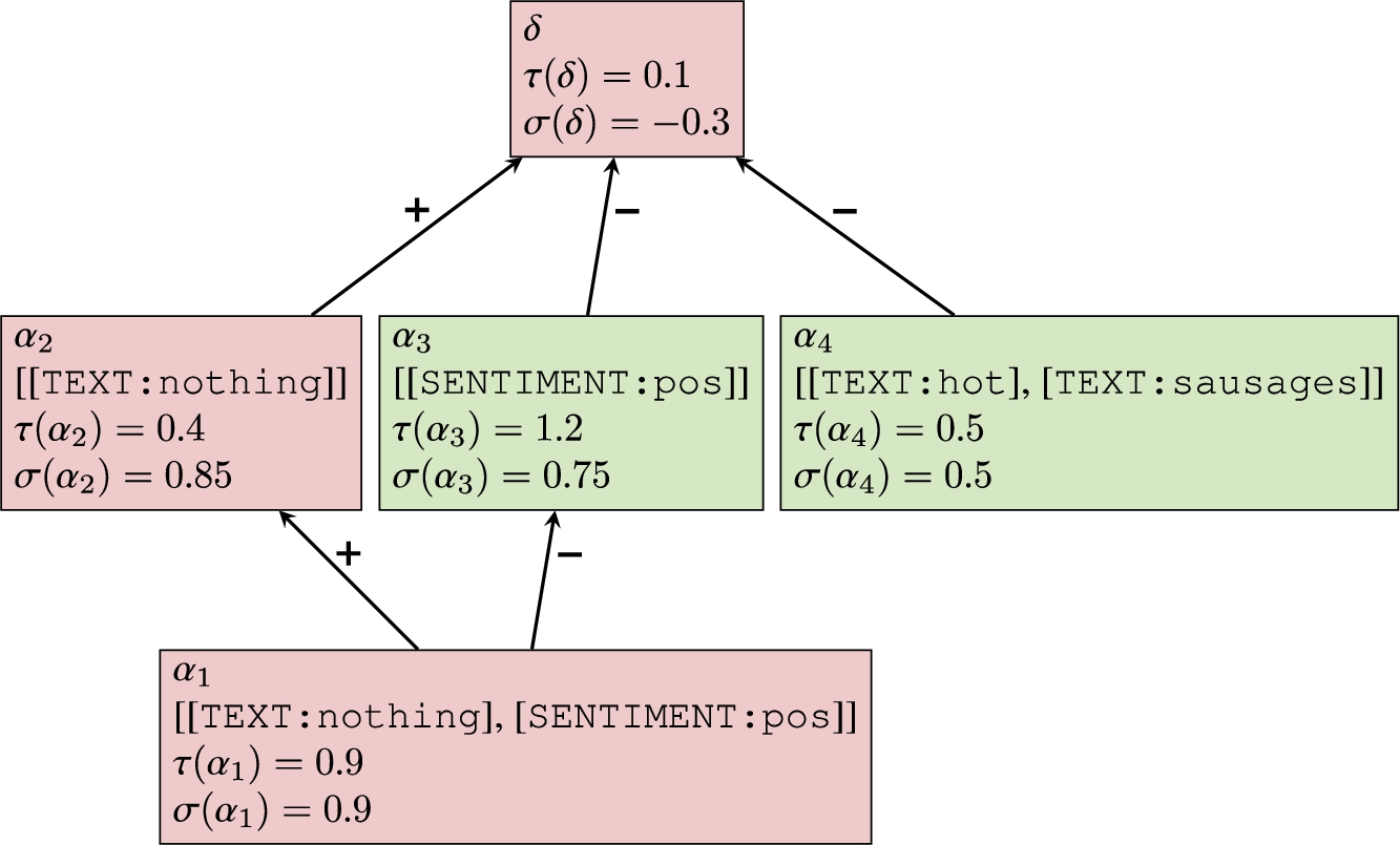
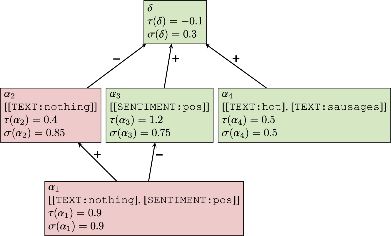
Fig. 6.

The extracted bottom-up QBAFc for the example in Fig. 2. The color represents the supported class (i.e., green for positive (1) and red for negative (0)). (The meaning of the equalities of the form τ(x)=v and σ(x)=v will be explained later.)

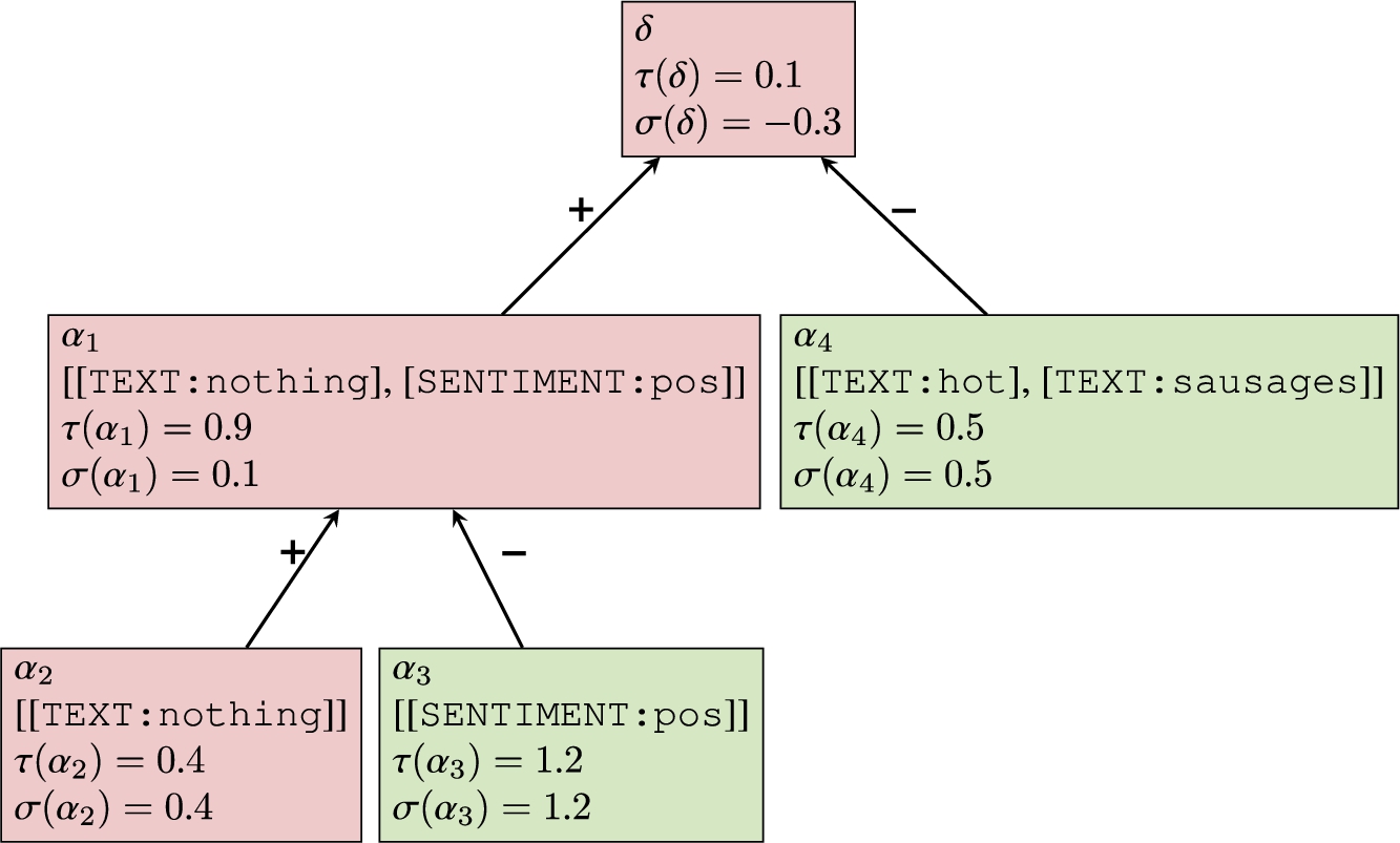
To explain, both the TQBAFc and the BQBAFc use the same A, τ, and c. Basically, each αi included in A is the argument drawn from pattern pi if it appears in x. So, if the input text x matches n patterns, A will have n+1 arguments. Amongst them, n arguments (those of the form αi) are for the n matched patterns, while the other one is for the default argument (δ) corresponding to the bias term b in the LR model. Therefore, the QBAFcs always have at least one argument, which is the default. The supported class (c) of each argument depends on whether the corresponding weight in the LR model is positive or negative. If wi is positive, it means that the existence of the pattern pi contributes to the positive class. So, the supported class of αi should be positive (1). For the default argument, we consider the sign of the bias term b instead. Because the supported class encapsulates the sign, the base score (τ) of the argument will be only the absolute value of the corresponding weight.

The extracted TQBAFc and BQBAFc for the example in Fig. 2 are shown in Figs 5 and 6, respectively. Following Definition 2, the differences between the TQBAFc and BQBAFc are the R− and R+ components. For the TQBAFc, (arguments for) more specific patterns attack or support (arguments for) more general patterns. The most general patterns, in turn, attack or support the default argument. Hence, the more general patterns will stay “closer” to the default argument (which is usually placed at the top of QBAFcs when using graphs to visualise them in figures) as shown in Fig. 5. That is why we call TQBAFcs top-down. Conversely, for the BQBAFc, (arguments for) more general patterns attack or support (arguments for) more specific patterns. The most specific patterns, in turn, attack or support the default argument. Therefore, the more specific patterns will stay “closer” to the default argument, as shown in Fig. 6, so we call BQBAFcs bottom-up. To decide whether two arguments are related by attack or support, we check the classes supported by the arguments: if they support the same class, then they are related by support; otherwise, by attack.

We proposed both the top-down and the bottom-up arrangements of QBAFcs as they are suitable for different situations. Later, in Section 6, we will show that, in TQBAFcs, we explain to users with general patterns first and provide more specific patterns as details when requested. In BQBAFcs, by contrast, we explain to users with specific patterns first (as they contain more information) and mention general patterns as supporting or opposing reasons.4 4

After this point, when we mention a QBAFc in this paper, we mean that it could be either a TQBAFc or a BQBAFc, unless otherwise stated. We assume that any generic QBAFc is of the form ⟨A,R−,R+,τ,c⟩. Furthermore, following notations in related work [7], we use R−(a) and R+(a) to represent sets of arguments attacking and supporting the argument a, respectively. Formally, R−(a)={b∈A|(b,a)∈R−} and R+(a)={b∈A|(b,a)∈R+}.

Lemma 2.

Given a QBAFc ⟨A,R−,R+,τ,c⟩, then δ∉R−(a) and δ∉R+(a) for all a∈A. So, the out-degree of δ is 0.

Indeed, we can see from RT−, RT+, RB−, and RB+ in Definition 2 that δ never attacks or supports any other argument. So, its out-degree equals 0, and therefore we usually put it at the top of figures (as shown in Figs 5 and 6).

Additionally, thanks to Definition 2 and Lemma 2, the graph structures underlying any TQBAFc and BQBAFc are directed acyclic graphs (DAGs).

Theorem 1.

The graph structure of any QBAFc is a directed acyclic graph (DAG).

Proof.

See Appendix A.2. □

4.2.Strength calculation

After we obtain the QBAFcs, the next step is to calculate the dialectical strength of each argument therein. To make this strength faithful to the underlying PLR model, we propose the logistic regression semantics, given by the strength function σ, defined next.

Definition 3.

The logistic regression semantics is defined as the strength function σ:A→R, where, for any a∈A:

(3)σ(a)=τ(a)+∑b∈R+(a)σ(b)ν(b)−∑b∈R−(a)σ(b)ν(b)

where τ(a) is the base score of a and ν(b) is the out-degree of b.

This semantics can be applied to both TQBAFcs and BQBAFcs. According to Equation (3), the strength of an argument starts from its base score, and it is increased and decreased by the strengths of its supporters and its attackers, respectively. However, the strength of each supporter/attacker must be divided by its out-degree (i.e., ν(b)) before being combined with the base score. Note that ν(b) in Equation (3) is always greater than or equal to 1 because b∈R−(a) or b∈R+(a), meaning that b attacks or supports at least one argument (which is a). So, no division by 0 may occur in this equation. Additionally, any argument a with no attackers or supporters (i.e., R−(a)=R+(a)=∅) will have the strength equal to its base score, by Definition 3.

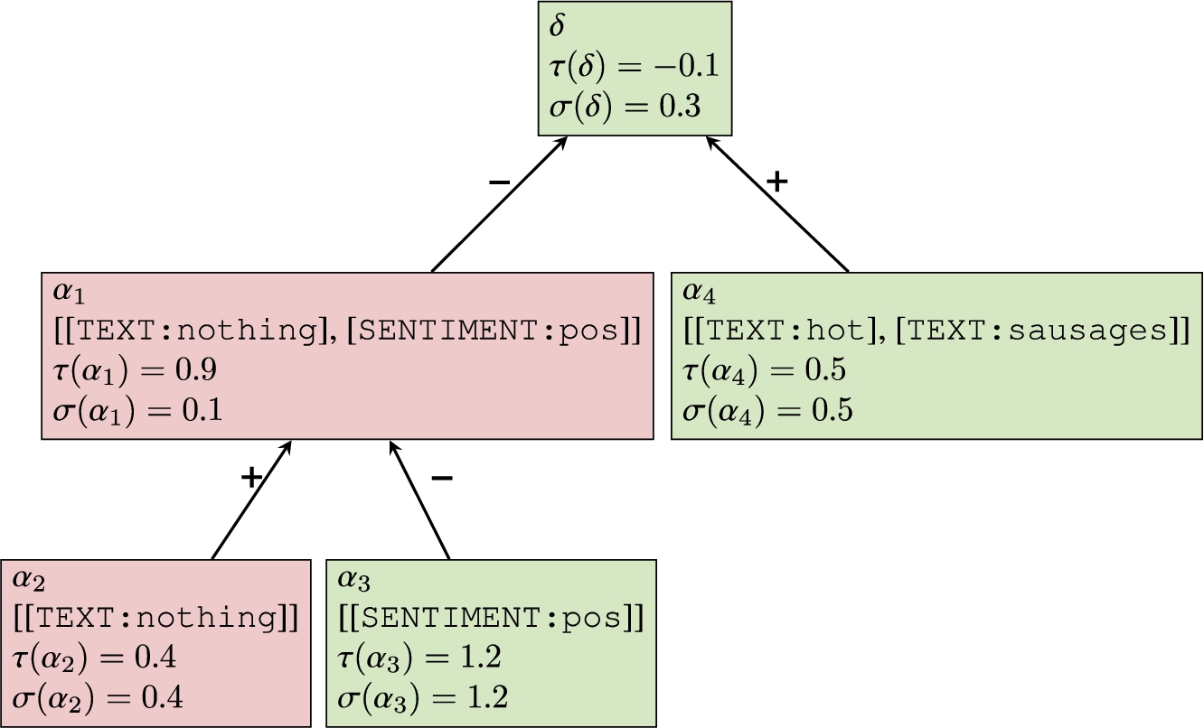
Because QBAFcs are DAGs (see Theorem 1), we can use topological sorting to define the order to compute the arguments’ strengths. Considering the TQBAFc in Fig. 5, for example, α1 and α4 do not have any attacker or supporter, so their strengths equal their base scores. Next, we can calculate the strengths of α2 and α3, and then δ:

σ(α2)=τ(α2)+∑b∈R+(α2)σ(b)ν(b)−∑b∈R−(α2)σ(b)ν(b)=0.4+∑b∈{α1}σ(b)ν(b)−∑b∈∅σ(b)ν(b)=0.4+0.92=0.85σ(α3)=τ(α3)+∑b∈R+(α3)σ(b)ν(b)−∑b∈R−(α3)σ(b)ν(b)=1.2+∑b∈∅σ(b)ν(b)−∑b∈{α1}σ(b)ν(b)=1.2−0.92=0.75σ(δ)=τ(δ)+∑b∈R+(δ)σ(b)ν(b)−∑b∈R−(δ)σ(b)ν(b)=0.1+∑b∈{α2}σ(b)ν(b)−∑b∈{α3,α4}σ(b)ν(b)=0.1+0.851−0.751−0.51=−0.3

All the results are displayed in Fig. 5. Similarly, the strengths are computed for the BQBAFc and shown in Fig. 6. We can see that the strength of the default arguments δ of both TQBAFc and BQBAFc is equal to the absolute of the logit ∑i=1dwifi+b of the PLR model.

Theorem 2.

For a given QBAFc, the prediction of the underlying PLR model can be inferred from the strength of the default argument:

(1) The predicted probability for the class c(δ) equals sigmoid(σ(δ)).
(2) Hence, if σ(δ)>0, the PLR model predicts class c(δ). Otherwise, it predicts the opposite class (i.e., 1−c(δ)).

Proof.

See Appendix A.3. □

In other words, we can read the prediction from the default argument δ. The negative strength of δ implies that the argument can no longer support its originally supported class; therefore, the prediction must be the opposite class. Since σ(δ) is computed from τ(δ) and the strengths of the attackers and the supporters of δ, we can use these attackers and supporters as explanation for the prediction. Furthermore, we may generalize the results of Theorem 2 to other arguments αi∈A. For instance, in Fig. 6, we could say that the pattern [[TEXT:nothing], [SENTIMENT:pos]] of α1 (weakly) supports the negative class with α1’s strength of 0.1, but it is not sufficient to make the final prediction become negative (indeed, even after the support by α1, the strength of δ remains negative, meaning that the final prediction is no longer the class δ originally supports, i.e., no longer the negative class).

4.3.Post-processing

We have shown how to extract QBAFcs, equipped with a suitable notion of dialectical strength to match the workings of PLR so as to serve as a basis for explanation thereof. Nevertheless, when arguments in these QBAFcs have a negative dialectical strength, the human interpretation of any resulting explanations may be difficult. Using Fig. 5 as an example, we can see that argument α2 ([[TEXT:nothing]]), supporting the negative class, supports argument δ, which represents the final prediction. Due to δ supporting the negative class and σ(δ) being negative, we can read from the figure that the final prediction is the positive class. However, it is counterintuitive to say that a pattern for the negative class supports the prediction of the positive class. Hence, we propose a post-processing step for QBAFcs to pave the way towards explanations better aligned with human interpretation.

Definition 4.

Given a QBAFc ⟨A,R−,R+,τ,c⟩ with σ(a) the dialectical strength of any a∈A, the corresponding post-processed QBAFc, denoted QBAFc′, is defined as ⟨A′,R−′,R+′,τ′,c′⟩ where

A′=A.
τ′:A→R and c′:A→{0,1} are defined such that, for each a∈A,
- ∗ If σ(a)⩾0, then τ′(a)=τ(a) and c′(a)=c(a).
- ∗ If σ(a)<0, then τ′(a)=−τ(a) and c′(a)=1−c(a).
R−′={(a,b)∈R−∪R+|c′(a)≠c′(b)∧σ(a)≠0}.
R+′={(a,b)∈R−∪R+|c′(a)=c′(b)∧σ(a)≠0}.

According to Definition 4, to post-process a QBAFc from the previous step, we change the supported class of arguments with negative strengths (σ(a)<0) to the other class (i.e., c′(a)=1−c(a)) and flip their base scores to be negative values (i.e., τ′(a)=−τ(a)). Then we re-label attacks and supports between arguments according to the new supported classes c′ while keeping the direction of the edges intact. Figures 7 and 8 show the post-processed QBAFcs of Figs 5 and 6, respectively. Note that, in this step, we also remove any edges where the strengths of the attackers or the supporters equal 0. As a result of this post-processing, the dialectical strength for all arguments becomes positive (as shown also in Figs 7 and 8). Generally:

Fig. 7.

The extracted top-down QBAFc in Fig. 5 after being post-processed.

Fig. 8.

The extracted bottom-up QBAFc in Fig. 6 after being post-processed.

Theorem 3.

Given a QBAFc ⟨A,R−,R+,τ,c⟩ and the corresponding QBAFc′ ⟨A′,R−′,R+′,τ′,c′⟩, using the logistic regression semantics σ, let σ(a) and σ(a)′ represent the dialectical strength of a∈A=A′ in QBAFc and QBAFc′, respectively. Then, the following statements are true:

If σ(a)⩾0, then σ(a)′=σ(a).
If σ(a)<0, then σ(a)′=−σ(a).

Proof.

See Appendix A.4. □

Corollary 1.

Given a QBAFc and the corresponding QBAFc′, σ(a)′=|σ(a)| for all a∈A=A′.

Furthermore, Theorem 2 also applies to QBAFc′s, as follows:

Corollary 2.

For a given QBAFc′, the prediction of the underlying PLR model is the class c′(δ) with the predicted probability of sigmoid(σ(δ)′).

Thus, intuitively, the effect of the post-processing step is to flip all the negative strengths to be positive, so we adjust the QBAFc accordingly, while preserving the interpretations of the arguments. For instance, if the original argument a has τ(a)=0.3, c(a)=1 and σ(a)=−0.5, the meaning is that the argument initially supports the positive class with the base score of 0.3, but after taking into account dialectical relations, it supports the negative class instead with strength 0.5. After post-processing, we will obtain τ′(a)=−0.3, c′(a)=0 and σ(a)′=0.5, with the (equivalent) meaning that the argument supports the negative class with strength 0.5.

5.Analyzing properties of QBAFc and QBAFc′

In this section, we analyze the logistic regression semantics σ, when applied to QBAFcs and QBAFc′s, according to 11 group properties of gradual semantics proposed in [7]. These properties have been used to evaluate many argumentation frameworks and semantics in the literature [3,52]. Moreover, these properties, or variants thereof, have been advocated as important when using argumentation as the basis for explanations [4,64], indicating that they lead to explanations that are consistent with general human reasoning and debate. Table 1 gives the formal definition of these properties for QBAFs ⟨A∗,R∗−,R∗+,τ∗⟩ under semantics σ∗. Note that these properties apply naturally to QBAFcs of the form ⟨A,R−,R+,τ,c⟩ and QBAFc′s of the form ⟨A′,R−′,R+′,τ′,c′⟩, under the LR semantics σ, for A∗=A or A∗=A′, R∗−=R− or R∗−=R−′, and so on. The definition of < between two sets used in GP10 and GP11 is defined as follows. Given P⊆A and Q⊆A, P⩽Q if and only if there exists an injective mapping f from P to Q such that ∀α∈P, σ(α)⩽σ(f(α)). Furthermore, P<Q if and only if P⩽Q but Q≰P.

Table 1

Dialectical properties for QBAFs ⟨A∗,R∗−,R∗+,τ∗⟩ under semantics σ∗ (adapted from [7])

GP1.	If R∗−(α)=∅ and R∗+(α)=∅, then σ∗(α)=τ∗(α).
GP2.	If R∗−(α)≠∅ and R∗+(α)=∅, then σ∗(α)<τ∗(α).
GP3.	If R∗−(α)=∅ and R∗+(α)≠∅, then σ∗(α)>τ∗(α).
GP4.	If σ∗(α)<τ∗(α), then R∗−(α)≠∅.
GP5.	If σ∗(α)>τ∗(α), then R∗+(α)≠∅.
GP6.	If R∗−(α)=R∗−(β), R∗+(α)=R∗+(β), and τ∗(α)=τ∗(β), then σ∗(α)=σ∗(β).
GP7.	If R∗−(α)⊂R∗−(β), R∗+(α)=R∗+(β), and τ∗(α)=τ∗(β), then σ∗(α)>σ∗(β).
GP8.	If R∗−(α)=R∗−(β), R∗+(α)⊂R∗+(β), and τ∗(α)=τ∗(β), then σ∗(α)<σ∗(β).
GP9.	If R∗−(α)=R∗−(β), R∗+(α)=R∗+(β), and τ∗(α)<τ∗(β), then σ∗(α)<σ∗(β).
GP10.	If R∗−(α)<R∗−(β), R∗+(α)=R∗+(β), and τ∗(α)=τ∗(β), then σ∗(α)>σ∗(β).
GP11.	If R∗−(α)=R∗−(β), R∗+(α)<R∗+(β), and τ∗(α)=τ∗(β), then σ∗(α)<σ∗(β).

Table 2

Summary of the group properties for gradual semantics [7] satisfied or unsatisfied by the logistic regression semantics σ when applied on QBAFcs and QBAFc′s

	GP1	GP2	GP3	GP4	GP5	GP6	GP7	GP8	GP9	GP10	GP11
⟨QBAFc,σ⟩	✔	✘	✘	✘	✘	✔	✘	✘	✔	✘	✘
⟨QBAFc′,σ⟩	✔	✔	✔	✔	✔	✔	✔	✔	✔	✘	✘

Table 2 summarizes our results (the proofs are in Appendix A.5). To briefly explain here, GP1 is satisfied by both ⟨QBAFc,σ⟩ and ⟨QBAFc′,σ⟩ because when there is neither attacker nor supporter, the right side of Equation (3) has only τ(α) left, making the argument’s strength equal its base score. Meanwhile, GP2-GP5 are not satisfied by ⟨QBAFc,σ⟩ since the strengths of attackers and supporters of QBAFc (not yet post-processed) could be negative. As a result, when an argument has only attackers, it may not be the case that its strength becomes lower than its base score (i.e., GP2 may not be satisfied). Similarly, when an argument has only supporters, it may not be the case that its strength becomes higher than its base score (i.e., GP3 may not be satisfied). Furthermore, the strength of an argument in ⟨QBAFc,σ⟩ could be less than its base score due to not only attackers with positive strengths but also supporters with negative strengths, making GP4 unsatisfied. Similarly, when the strength of an argument in ⟨QBAFc,σ⟩ is higher than its base score, it could also be due to attackers with negative strengths (not only supporters with positive strengths), making GP5 unsatisfied. In contrast, after we post-process QBAFc to be QBAFc′, no argument strengths can be negative (see Corollary 1); therefore, GP2-GP5 are satisfied by ⟨QBAFc′,σ⟩. Next, GP6 and GP9 are satisfied by both ⟨QBAFc,σ⟩ and ⟨QBAFc′,σ⟩ as we can easily see from Equation (3). As for GP2-GP5, GP7 and GP8 may not be satisfied by ⟨QBAFc,σ⟩ due to the fact that, in QBAFc, the strengths of attackers and supporters could be negative, whereas ⟨QBAFc′,σ⟩ satisfies GP7 and GP8 since QBAFc′ does not suffer from negative strengths. Lastly, both ⟨QBAFc,σ⟩ and ⟨QBAFc′,σ⟩ do not satisfy GP10 and GP11 because the < relation imposes a condition only on argument strengths while our semantics σ considers not only the strengths of the attackers and the supporters but also their out-degrees. For illustrative counterexamples of these GPs, please see Appendix A.5.

In conclusion, ⟨QBAFc′,σ⟩ satisfies nine out of the eleven group properties, while ⟨QBAFc,σ⟩ satisfies only three. This means that our post-processing step is important to make the argumentation framework align better with human interpretation and become more suitable for generating local explanations.

6.Presenting AXPLR to humans

Presenting the whole QBAFc′ as a local explanation to lay users may not be a good idea since the graph could be very complicated (in terms of the number of arguments, relations, and depth). Also, the notions of attack and support may not be familiar to the users. So, the last step of AXPLR is extracting the explanation from the QBAFc′. We know from Theorem 2 and Corollary 2 that the prediction of the LR model is associated to the strength of the default argument δ. Hence, we can explain the prediction based on how σ(δ)′ was calculated. The value of σ(δ)′ depends on τ′(δ) (corresponding to the bias term in LR) and the strength σ of all the attackers and supporters of δ. Therefore, we return, as the local explanation for c′(δ), a list of triplets (pj,π(pj,x),σ(αj)′) where x is the input text, αj (representing the pattern pj) is one of the k strongest supporters of δ, and π(pj,x) is a part of x that matches the pattern pj. If we want both evidence for and counter-evidence against the prediction, we can show triplets (pj,π(pj,x),σ(αj)′) for the top k supporters and attackers with the highest σ(αj)′. We call explanations of this form shallow AXPLR. Figure 9 shows an example of shallow AXPLR (extracted from a BQBAFc′) for the deceptive review detection task5 5 where the color intensity represents the strengths of the arguments. Shallow AXPLR are similar to the flat logistic regression explanations (FLXs) introduced in Section 2.4. The only differences are that (i) FLXs select the top k patterns based on the size of wjfj (which is equivalent to τ(αj)) while our shallow AXPLR select top k arguments based on the dialectical strength σ(αj), and (ii) any patterns matched in x can be in FLXs whereas only attackers and supporters of δ can be in shallow AXPLR.

Fig. 9.

Example of shallow AXPLR for deceptive review detection. The partial input text and the model prediction are shown in the top-most box. The shallow AXPLR shows evidence for both the deceptive class and the truthful class. The patterns shown correspond to strongest supporters and attackers of δ. The meaning of each pattern/argument is also provided. The color and its intensity represent the supported class and the strengths of the arguments, respectively.

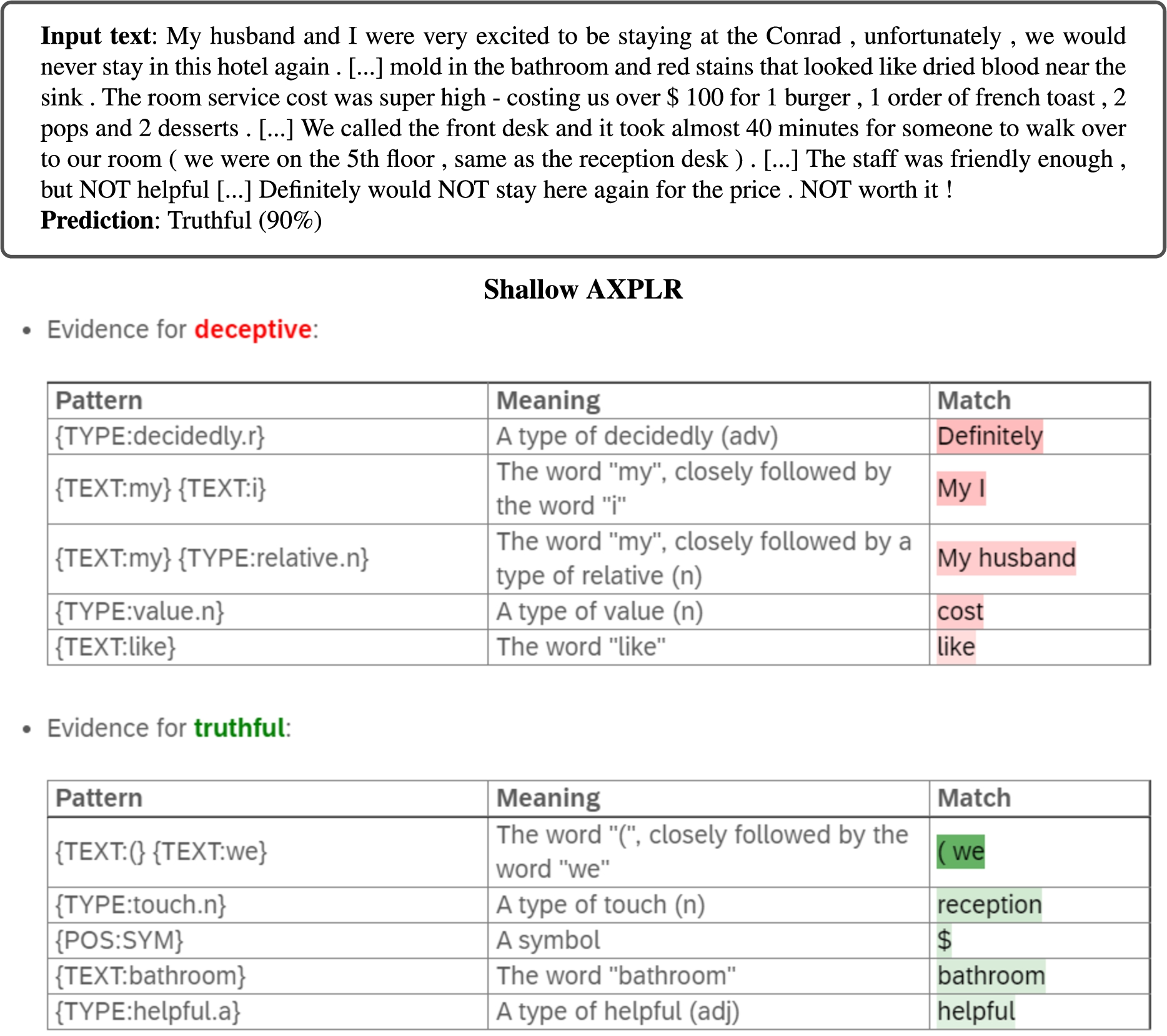
Shallow AXPLR leverage only the attackers and supporters of δ, but ignores the additional information available in the QBAFc′. Therefore, we propose another variation of AXPLR, called deep AXPLR, which also use other arguments and relations in the QBAFc′. Basically, deep AXPLR expand shallow AXPLR by additionally allowing users to see attackers and supporters (if any) of arguments in shallow AXPLR as well as “deeper” arguments in the QBAFc′ until there is no attacker or supporter for those arguments. Figure 10 shows a deep AXPLR, explaining the same example and using the same BQBAFc′ as the shallow AXPLR in Fig. 9 does. Note that a deep AXPLR from a BQBAFc′ (as in Fig. 10) shows specific patterns to the users first (as they directly support or attack δ) and hides more general patterns as supporting or opposing reasons (to be expanded) in deeper levels. In contrast, due to the opposite way of drawing attacks and supports, a deep AXPLR from a TQBAFc′ explains to users with general patterns first and provides more specific patterns as expandable details in deeper levels.

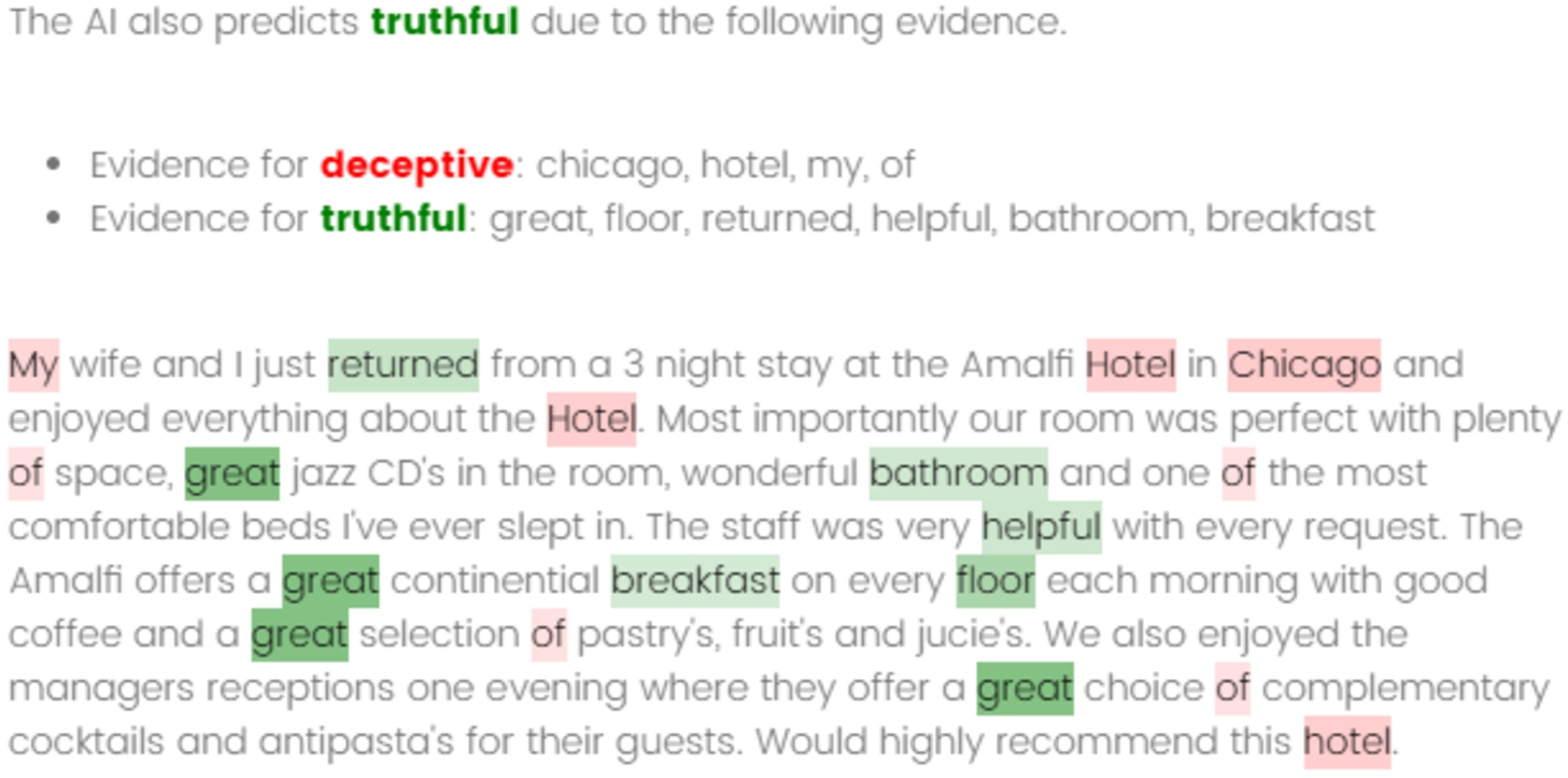
Fig. 10.

Example of deep AXPLR for deceptive review detection. The partial input text and the model prediction are shown in the top-most box. The deep AXPLR shows evidence for both the deceptive class and the truthful class. A user can expand some patterns/arguments to see their sub-patterns (i.e., their attackers and/or supporters) such as, on the left, [[TEXT:i]] and [[TEXT:like]] supporting [[TEXT:like], [TEXT:i]]. The meaning of each pattern is provided as a tooltip. The color and its intensity represent the supported class and the strengths of the arguments, respectively.

Shallow and deep AXPLR are just two examples of explanations that can be drawn from QBAFc′s. We leave the study of other forms of explanations, such as conversational explanations [11] and counterfactual explanations [2], for future work.

7.Experimental setup

To evaluate AXPLR, we conducted both empirical and human evaluations. For the empirical evaluation, we calculated some statistics for the QBAFc′s extracted for target examples and performed analyses concerning sufficiency of the generated explanations (see Section 8). For the human evaluation, we (i) assessed plausibility of the explanations, i.e., how well the explanations from AXPLR align with human explanations compared to a standard method for explaining LR results (see Section 9), and (ii) assessed how well AXPLR can teach and support humans to perform a new task (see Section 10).6 6

In the experiments, we targeted binary text classification using three English datasets as shown in Table 3. The table also shows the classes we consider as positive and negative when running GrASP and AXPLR and the number of examples for each data split (used for training, developing, and testing the models; please see Appendix B for more details about these splits). Specifically, the datasets are:

SMS Spam Collection [5] focusing on detecting spams in a collection of SMS (short message service) messages. The dataset is imbalanced, containing 13.40% spam messages and 86.60% ham messages (i.e., non-spams).
Amazon Clothes [23], focusing on classifying whether a review (of clothing, shoes, and jewelry products) has positive or negative sentiment. The overall dataset is balanced.
Deceptive Hotel Reviews [48,49] focusing on identifying whether a given hotel review is truthful (genuine) or deceptive (fake). There are 1600 reviews in total for 20 hotels. For each hotel, there are 20 truthful positive, 20 truthful negative, 20 deceptive positive, and 20 deceptive negative reviews (positive and negative here refer to the review sentiment).

Table 3

Datasets used in the experiments

Dataset	Positive class	Negative class	Training / Development / Testing
SMS Spam Collection	Spam	Not spam	3567 / 892 / 1115
Amazon Clothes	Positive	Negative	3000 / 300 / 10000
Deceptive Hotel Reviews	Deceptive	Truthful	1024 / 256 / 320

For the LR classifiers of the first two datasets, the GrASP patterns were constructed with lemma, part-of-speech tags (POS), wordnet hypernyms, and sentiment attributes. We used alphabet size of 200, allowed two gaps in the patterns, and generated 100 patterns in total. For the last dataset (Deceptive Hotel Reviews), the settings were the same except that we used text attributes (capturing the whole word) instead of the lemma attributes and we generated 200 patterns in total. The performance of the LR classifiers of the three datasets are reported in Table 4. Accuracy is the percentage of correct predictions on the test set, while F1 is a harmonic mean of Precision and Recall of the model. Positive F1 and Negative F1 are F1s when we consider the positive and the negative classes as the main class. These two F1s are then averaged to be Macro F1. For more details about the evaluation metrics, please see Appendix B.

Table 4

Performance of the pattern-based LR models on the test sets

Dataset	Positive F1	Negative F1	Macro F1	Accuracy
SMS Spam Collection	0.891	0.986	0.939	0.975
Amazon Clothes	0.836	0.836	0.836	0.836
Deceptive Hotel Reviews	0.847	0.859	0.853	0.853

8.Experiment 1: Empirical evaluation

We divide the empirical evaluation into two parts. The first part discusses the statistics for QBAFc′s we generated from the test sets. This helps us understand what the argumentation graphs look like on average. The second part focuses on sufficiency, aiming to answer “How many supporting arguments are needed on average so as to sufficiently make the model predict what it predicts?”. This helps us decide how many arguments we should show in AXPLR generally. It is noteworthy that, although we conducted Experiment 1 on the three chosen datasets, the way of reading and interpreting QBAFc′ statistics discussed in this section can be applied to understand PLR models trained on other datasets too. The core contribution of this section is not to show that AXPLR outperforms other explanation methods, but to show that we can better understand the global behavior of the PLR model by interpreting statistics of the extracted QBAFc′s.

8.1.Statistics for QBAFc′s

Table 5 shows the statistics of the QBAFc′s for the SMS Spam Collection, Amazon Clothes, and Deceptive Hotel Reviews datasets. In particular, we count the total number of arguments in each QBAFc′ as well as the number of arguments supporting positive and negative classes (A+,δ and A−,δ respectively, defined below) and then compute the average and the standard deviation across all the test examples.

A+,δ={a∈A|c(a)=1}A−,δ={a∈A|c(a)=0}

We consider both the statistics for the whole test sets and the statistics for each of the four possible situations – true positives (TP), true negatives (TN), false positives (FP), and false negatives (FN). TP and TN are the cases where the model correctly predicts that the true class is 1 and 0, respectively. FP refers to cases when the predicted label is 1 but the true label is 0. On the contrary, FN refers to cases when the predicted label is 0 but the true label is 1. For more details, please see Appendix B.

Table 5

Statistics (Average ± SD) of QBAFc′ for the SMS Spam Collection, Amazon Clothes, and Deceptive Hotel Reviews dataset. A+,δ, A−,δ are sets of arguments supporting positive and negative classes, respectively. TP, TN, FP, and FN stand for true positives, true negatives, false positives, and false negatives, respectively. The number of examples for each case as well as the total number of examples are indicated in the last row of the table

Dataset	SMS Spam Collection		Amazon Clothes		Deceptive Hotel Review

Measurement	TQBAFc′	BQBAFc′	TQBAFc′	BQBAFc′	TQBAFc′	BQBAFc′
\|A\|	10.08 ± 11.55	10.08 ± 11.55	16.09 ± 8.13	16.09 ± 8.13	19.44 ± 6.82	19.44 ± 6.82
– TP	35.98 ± 12.26	35.98 ± 12.26	14.85 ± 7.57	14.85 ± 7.57	19.54 ± 6.54	19.54 ± 6.54
– TN	6.66 ± 6.01	6.66 ± 6.01	17.45 ± 8.21	17.45 ± 8.21	20.24 ± 6.86	20.24 ± 6.86
– FP	36.00 ± 11.98	36.00 ± 11.98	14.99 ± 8.14	14.99 ± 8.14	17.77 ± 6.48	17.77 ± 6.48
– FN	19.30 ± 9.66	19.30 ± 9.66	16.57 ± 9.31	16.57 ± 9.31	15.48 ± 7.34	15.48 ± 7.34
\|A+,δ\|	6.25 ± 7.77	6.47 ± 8.07	7.45 ± 4.50	7.43 ± 4.88	9.89 ± 5.02	10.34 ± 5.00
– TP	24.68 ± 7.70	25.42 ± 7.52	9.74 ± 4.07	10.22 ± 4.51	13.58 ± 4.53	13.85 ± 4.50
– TN	3.85 ± 3.69	4.00 ± 4.01	5.20 ± 3.76	4.75 ± 3.68	6.92 ± 3.21	7.43 ± 3.32
– FP	22.20 ± 6.87	24.20 ± 6.02	8.47 ± 4.12	8.49 ± 4.34	10.77 ± 3.74	11.42 ± 4.09
– FN	11.74 ± 4.83	12.48 ± 5.69	6.10 ± 4.29	5.84 ± 4.37	6.29 ± 3.61	7.10 ± 3.96
\|A−,δ\|	3.83 ± 4.14	3.61 ± 3.81	8.64 ± 5.89	8.65 ± 6.24	9.55 ± 5.33	9.10 ± 5.13
– TP	11.30 ± 5.37	10.57 ± 5.41	5.10 ± 4.18	4.63 ± 4.27	5.96 ± 3.14	5.69 ± 2.93
– TN	2.81 ± 2.65	2.66 ± 2.33	12.25 ± 5.36	12.71 ± 5.53	13.32 ± 4.81	12.81 ± 4.68
– FP	13.80 ± 5.50	11.80 ± 6.06	6.52 ± 4.38	6.50 ± 4.44	7.00 ± 3.27	6.35 ± 2.86
– FN	7.57 ± 5.29	6.83 ± 4.25	10.47 ± 5.49	10.73 ± 5.57	9.19 ± 4.19	8.38 ± 3.77
# Examples	1115 (TP: 115, TN: 972, FP: 5, FN: 23)		10000 (TP: 4176, TN: 4186, FP: 848, FN: 790)		320 (TP: 130, TN: 143, FP: 26, FN: 21)

According to Table 5, the spam dataset had the minimum average number of arguments (∼10 arguments per example as shown by |A| in the table). However, if we look at examples for which the prediction is positive (i.e., both TP and FP), we find 36 arguments per example on average. Looking at the underlying PLR model, we found that the default argument δ before post processing supported the negative class with τ(δ)=5.800 (not shown in the table), which was very high compared to the base scores of other arguments. This means that the classifier answered “Not spam” by default unless it could identify sufficient evidence (i.e., certain patterns found in the input text) to answer “Spam”. Even true negative examples (TN) had around three arguments for the negative class on average, including δ. Interestingly, false negative examples (FN) had a relatively higher number of arguments than true negatives, but still less than those of true positives (TP). This implies that the false negative examples usually had some, but insufficient, evidence for the positive class, compared to the true negatives which almost have nothing.

Unlike the SMS Spam Collection dataset, the base scores of δ for the Amazon Clothes and the Deceptive Hotel Reviews datasets were 0.2597 and 0.6932 supporting the negative class, respectively (not shown in the table). In order to push the prediction to either positive or negative, we needed evidence. Hence, for these two datasets, the average number of arguments were similar for both classes (as shown by |A| of TP, TN, FP, FN in Table 5). Examples predicted as positive, therefore, had higher number of arguments for the positive class (|A+,δ|) than those predicted as negative. Similarly, examples predicted as negative had higher number of arguments for the negative class (|A−,δ|) than those predicted as positive.

In conclusion, the statistics of QBAFc′ reported here can help us understand the global behavior of the underlying PLR model (e.g., conditions for it to predict positive or negative). We noticed a glimpse of default reasoning our spam classifier behaves. This, moreover, reveals a weakness of the model: it is susceptible to short spam texts which usually have insufficient number of arguments for the positive (spam) class due to the limited text length. In contrast, the PLR models for the other two tasks do not employ default reasoning extensively. The models require sufficient evidence from an input text to predict either class.

8.2.Sufficiency

Next, given a QBAFc′, we were interested in the number of supporting arguments needed in order to sufficiently explain the prediction. Here, sufficiently means that given the base score of δ and all the attacking arguments, the strengths given by these supporting arguments are enough to make the strength of δ greater than 0. In other words, for each test example, we wanted to find the smallest k such that S⊆R+′(δ), |S|=k and

(4)τ′(δ)+∑b∈Sσ(b)ν(b)−∑b∈R−′(δ)σ(b)ν(b)>0

Furthermore, we extended our question to other arguments in QBAFc′ which had at least one attacker or supporter. (We call them intermediate arguments.) We wondered how many supporting arguments were needed to make the strength of the argument greater than 0, taking into account the base score and all the strengths from the attackers. Knowing the answers to these questions helps us decide how many arguments we should show to the users for explaining the final prediction or the intermediate arguments.

Table 6

The smallest number of supporting arguments k which are sufficient to make the strength of the default argument δ greater than 0 for 80% and 100% of δ from all the test examples. We consider both TQBAFc′ and BQBAFc′ and, specifically, when the final supported class of δ is and is not the original supported class of δ before the post-processing step

Consider	TQBAFc′						BQBAFc′

	All δ		c′(δ)=c(δ)		c′(δ)≠c(δ)		All δ		c′(δ)=c(δ)		c′(δ)≠c(δ)

Sufficient for	80%	100%	80%	100%	80%	100%	80%	100%	80%	100%	80%	100%
SMS Spam.	0	7	0	1	4	7	0	11	0	7	6	11
Amazon Clothes	2	9	2	9	1	3	3	15	3	15	3	12
Deceptive Review.	4	10	4	9	4	10	4	11	4	11	4	9

Table 7

The smallest number of supporting arguments k which are sufficient to make the strength of intermediate arguments α greater than 0 for 80% and 100% of intermediate arguments from all the test examples. We consider both TQBAFc′ and BQBAFc′ and, specifically, when the final supported class of α is and is not its original supported class before the post-processing step

Consider	TQBAFc′						BQBAFc′

	All α		c′(α)=c(α)		c′(α)≠c(α)		All α		c′(α)=c(α)		c′(α)≠c(α)

Sufficient for	80%	100%	80%	100%	80%	100%	80%	100%	80%	100%	80%	100%
SMS Spam.	0	5	0	4	2	5	1	2	0	1	1	2
Amazon Clothes	0	4	0	2	1	4	0	2	0	1	1	2
Deceptive Review.	0	2	0	1	1	2	1	3	0	1	1	3

Because different arguments could have different values of k that satisfy the sufficiency condition in Equation (4), we consider the values k which are sufficient for 80% and 100% of the arguments for each dataset. Tables 6 and 7 show the results for the default arguments δ and the intermediate arguments αi, respectively. Considering the sufficiency for δ in Table 6, we can see that the numbers of supporting arguments needed were different for each dataset. The SMS Spam Collection dataset seemed to need the least. However, this was the case only for examples with c′(δ)=c(δ), i.e., the supported class after post-processing was the same as the original class δ supports. The reason was that the base score of δ was relatively high. It could outnumber the strengths from the attackers even without the strengths from the supporters. Nevertheless, this was not true when the supported class changed (i.e., c′(δ)≠c(δ)) as it required 4–6 supporting arguments to make 80% of the test set have sufficient explanations. Meanwhile, the Amazon Clothes and the Deceptive Hotel Reviews datasets required approximately 1–3 and 4 supporting arguments, respectively, for sufficient explanations of 80% of the test set (regardless of the predicted class).

Additionally, for δ of the SMS Spam Collection and the Amazon Clothes datasets, BQBAFc′ required more supporting arguments than TQBAFc′. This was likely because BQBAFc′ connected the arguments representing the most specific patterns to the default. For these two datasets, they outnumbered the most general patterns TQBAFc′ connected to the default. So, the default argument of BQBAFc′ had more supporters where the strengths were distributed. Therefore, more supporters were required to make the sufficient explanation.

Considering the sufficiency for intermediate arguments α in Table 7, only one supporting argument was usually sufficient to explain the supported class. Even without any supporters, only the base score was sufficient in most cases if the supported class is not flipped after post-processing (i.e., c′(α)=c(α)). Hence, if a user wants to see supporting information for an intermediate argument, when the space is limited, showing only 1–2 supporters are totally acceptable.

To sum up, the key finding from this sufficiency analysis is threefold. First, the number of supporting arguments required for the default argument varies for each task and predicted class. Second, using BQBAFc′ often requires more supporting arguments than TQBAFc′ as δ of BQBAFc′ has more supporters (i.e., more specific patterns) connected to it where the strengths were distributed. Third, it is usually sufficient to show only 1–2 supporters for intermediate arguments α. To further support these key findings, we present plots between k and the percentage of arguments where k can satisfy the sufficiency condition in Appendix D.

9.Experiment 2: Plausibility

In this section, we aimed to evaluate the plausibility of AXPLR, compared to FLX, to confirm our hypothesis that it is essential to consider relations between features (i.e., patterns) when we generate local explanations. So, we compared the feature scores given by the explanation methods to scores reflecting how humans consider the features. For instance, if a machine indicates pattern p1 as a main reason for predicting the positive class and humans think that p1 is truly a sign of the positive class, we can say that the machine explanation aligns well with human judgement (i.e., having high plausibility). In other words, the higher correlation between machine explanation scores and human scores implies the higher plausibility of the explanation method. Hence, we chose Pearson’s correlation as the metric in this experiment.

9.1.Datasets

We used the SMS Spam Collection (spam filtering) and the Amazon Clothes (sentiment analysis) datasets since humans generally perform well on these two tasks, making the human scores reliable. For each dataset, we needed 500 test examples for evaluation. These examples must have at least one pattern matched (so that the explanation contains at least one pattern to be investigated), and they must have the predicted probability of the output class greater than 0.9 to ensure that the bad quality of the explanation was not due to low model accuracy or text ambiguity. Note that we did not conduct this experiment on the Deceptive Hotel Reviews dataset as lay humans are not adept at identifying deceptive reviews. The human accuracy was only around 55% in [34], so we cannot trust human judgement on machine explanations in this task. We would work on the deceptive review detection task in the next experiment instead.

9.2.Machine explanations

As discussed in Section 6, both FLX and AXPLR use (pj,π(pj,x),sj) triplets as explanations where sj is the score of the pattern pj or the match π(pj,x) in the input x. For FLX, sj equals wjfj, and any pj with the relatively large score sj can be chosen as a part of the explanation. By contrast, shallow AXPLR uses only arguments at the top level of the underlying QBAFc, i.e., arguments attacking or supporting δ, as explanations. Meanwhile, deep AXPLR can use any arguments in the QBAFc. The sj of AXPLR also depends on whether the QBAFc is TQBAFc or BQBAFc. So, we compared all of these variations in this experiment. Note that, because τ′ and σ of AXPLR need to be interpreted with the supported class, we adjusted sj for AXPLR to be self-contained. To put it simply, we multiplied τ′(αj) and σ(αj)′ of AXPLR with 1 if c′(αj)=1, or with −1 if c′(αj)=−1. This made the higher sj always imply the stronger evidence for the positive class (similar to FLX).

9.3.Human scores

We recruited human participants via Amazon Mechanical Turk (MTurk)7 7 and asked them whether the pattern pj or the matched phrase π(pj,x) was the evidence for the positive or the negative class. Since the pattern pj only may be difficult to understand, we provided the translation to help lay users on MTurk, as shown in Fig. 11 (a). Another way to present the pattern is to show samples of phrases (from the training set) matched by the pattern. We also collected human answers for this pattern representation showing five unique samples per pattern,8 8 as displayed in Fig. 11 (b). Finally, a question for a single matched phrase π(pj,x) was a lot simpler as shown in Fig. 11 (c). We provided five options for each question, ranging from definitely positive, positive, not sure, negative, and definitely negative. These correspond to the score 2, 1, 0, −1, and −2, respectively. For the SMS Spam Collection dataset, these options were instead definitely spam, spam, not sure, non-spam, and definitely non-spam.

For each dataset, since there are only 100 distinct patterns, we needed 100 questions for patterns and another 100 questions for groups of sample phrases of those patterns. However, the numbers of matched phrases are different between the two datasets. The SMS Spam Collection test samples had 2,964 distinct matched phrases in total, while the Amazon Clothes test samples had 3,140 distinct matched phrases. Considering both datasets and all the three types of questions, we had (100 + 100 + 2,964) + (100 + 100 + 3,138) = 6,502 distinct questions. Each distinct question was answered by five participants, and the scores were averaged before comparing with machine explanation scores. In other words, we can read the Pearson’s correlations as the degree of alignment between machine explanations and the average of the human annotations. Concerning the payment for answering questions, we paid the participants $0.30 per 10 pattern questions, $0.20 per 10 group-of-phrases questions, and $0.20 per 20 matched phrase questions.

Fig. 11.

Examples of questions (from the Amazon Clothes dataset) posted on Amazon Mechanical Turk to elicit human scores.

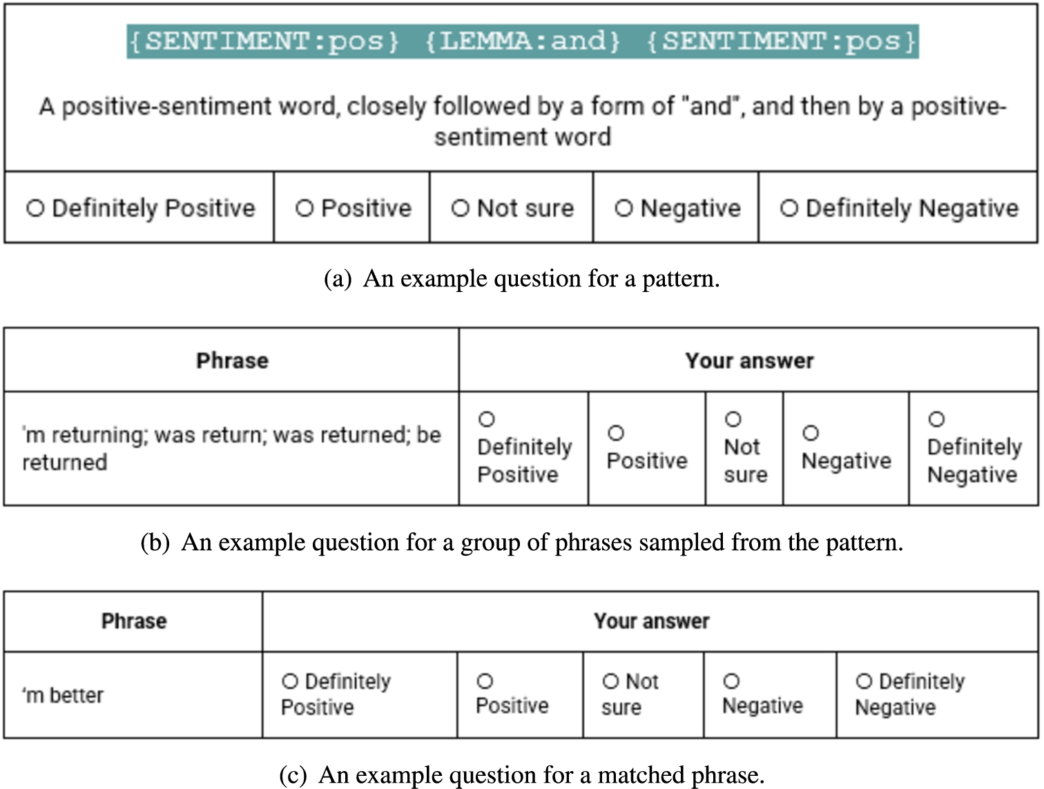
Table 8

Pearson’s correlation between explanation scores and human scores for the SMS Spam Collection dataset

Explanation scores	Human scores

	Pattern	Samples	Matched Phrase
FLX	0.227	0.175	−0.022
TQBAFc′
sj=τ′(αj) (top level)	0.687	0.533	−0.019
sj=σ(αj)′ (top level)	0.520	0.462	0.125
sj=σ(αj)′ (all levels)	0.176	0.100	0.005
BQBAFc′
sj=τ′(αj) (top level)	0.197	−0.005	−0.047
sj=σ(αj)′ (top level)	0.240	0.175	0.046
sj=σ(αj)′ (all levels)	0.271	0.308	0.053
Fleiss κ with five answer categories	0.001	0.068	0.118
Fleiss κ with three answer categories	−0.003	0.085	0.192

Table 9

Pearson’s correlation between explanation scores and human scores for the Amazon Clothes dataset

Explanation scores	Human scores

	Pattern	Samples	Matched Phrase
FLX	0.503	0.525	0.529
TQBAFc′
sj=τ′(αj) (top level)	0.423	0.491	0.487
sj=σ(αj)′ (top level)	0.632	0.693	0.688
sj=σ(αj)′ (all levels)	0.490	0.503	0.501
BQBAFc′
sj=τ′(αj) (top level)	0.442	0.466	0.486
sj=σ(αj)′ (top level)	0.599	0.621	0.634
sj=σ(αj)′ (all levels)	0.610	0.627	0.627
Fleiss κ with five answer categories	0.210	0.297	0.357
Fleiss κ with three answer categories	0.369	0.533	0.563

9.4.Results

Tables 8 and 9 report the Pearson’s correlations between the machine explanation scores and the human scores collected from Amazon Mechanical Turk for both datasets. The bottom part of each table shows inter-rater agreement metrics to reflect the agreement among annotators for each pair of dataset and question type. Because different questions may be answered by different sets of individuals, we chose Fleiss’ kappa [19] as the inter-rater agreement metric in this experiment. Considering five answer options (categories) as explained in Section 9.3, we observe that the agreement metrics for the SMS Spam Collection dataset were very close to zero (especially for the questions for patterns and samples), while the agreement rates for the Amazon Clothes dataset (sentiment analysis task) were noticeably higher. Even though the Fleiss’ kappa metrics of the latter task (with five answer categories) are around 0.210–0.357, we noticed that the different human annotations for the same pattern/phrase usually belong to the same polarity but with different degrees such as a phrase getting three “Definitely negative” and two “Negative” from five annotators. Hence, we calculated the Fleiss’ kappa again but now based on the answer polarity only. Specifically, we considered “Definitely negative” and “Negative” to be a single answer category and considered “Definitely positive” and “Positive” to be another answer category. Together with the “Not sure” option, we had three answer categories, and we then reported the resulting Fleiss’ kappa in the last row of Table 9. With a similar way of grouping answer options, the last row of Table 8 shows the Fleiss’ kappa when considering three answer categories for the SMS spam detection task (i.e., “Spam”, “Not spam”, and “Not sure”). We can see that even considering three answer categories does not help the SMS spam detection task, confirming that their human answers are unreliable. On the contrary, the Fleiss’ kappa scores are significantly stronger for the sentiment analysis task (Amazon Clothes dataset) if we consider only three answer categories, confirming that human answers in this task are reliable. This was likely because evidence from the sentiment analysis task (including patterns, samples, matched phrases) usually conveys clear meanings even without contexts, whereas evidence from the spam detection task often requires contexts for humans to make decisions. For example, upset, worthless, and disappointed were surely for negative reviews. In contrast, mobile, win, and call could appear both in spam and non-spam texts. This caused higher disagreements in human answers though the model used these words certainly as evidence for the spam class. As a result, the human scores for the spam task were less reliable than the scores for the sentiment analysis task. Consequently, the overall correlations in Table 8 were also less than the scores in Table 9.

Hence, we focused on discussing the results in Table 9 with more reliable human scores. For each row, the correlation between the explanations and the (average) human scores for patterns was lower than for samples and matched phrases. Therefore, we should show not only the patterns but also some matched samples of the patterns to generate better plausible explanations. In addition, for TQBAFc′ and BQBAFc′, the strengths of top-level arguments σ(αj)′ were better than the base scores τ′(αj) in terms of the alignment with human judgement. The correlations were also significantly higher than FLX. This confirmed the advantage of the prominent feature of AXPLR, i.e., considering interactions between patterns when generating local explanations. However, by extending from arguments in the top level to all levels in the QBAFc′, only the correlations in BQBAFc′ remained high, while the correlations in TQBAFc′ dropped. Therefore, deep AXPLR, utilizing arguments of all levels in the graph, would go along better with BQBAFc′ than TQBAFc′. It also implied that the base scores of the most specific patterns, which equaled their strengths in TQBAFc′, required some adjustments to align well with human judgement.

9.5.Summary and discussion

In this experiment, we showed that the calculated strengths σ(αj)′ outperformed the FLX baseline and QBAFc′ using base scores τ′(αj) significantly, with a 0.10–0.20 absolute difference in correlations for top-level arguments of QBAFc′ and all-level arguments of BQBAFc′ in particular, confirming the capability of our approach. However, it is noteworthy that a perfect correlation is hardly possible to obtain in this experiment because of two reasons. First, we constructed relations among patterns based on their specificity (see Definition 1) only, whereas there could be other associations among patterns that go beyond pattern matching specificity such as semantic relations, which are more difficult to identify and quantify. We hope that our work will inspire future research to investigate these subtle relations. Second, it is possible that the model relied on patterns that humans do not use but such patterns coexist with a specific class in the training data often enough for the model to leverage them. This problem is called spurious correlations, which is a challenging problem in natural language processing [68,69]. In other words, the perfect correlation between machine explanation scores and human scores can hardly be achieved also because the machine indeed reasons in a different way from what humans generally do.

10.Experiment 3: Tutorial and real-time assistance

Among the three datasets, the deceptive review detection task is the most difficult tasks for humans. When a trained model is more effective than humans in a particular task, it would be beneficial for humans to learn insights or tricks from the model, and explanations pave the way towards the learning as they reveal how the model works to humans. In this experiment, therefore, we follow the study [34] to evaluate how effective AXPLR can be used to teach and support humans to perform deceptive review detection.

10.1.Setup

We recruited participants via Amazon Mechanical Turk and redirected them to our a survey created using Qualtrics.9 9 The survey aimed to assess the capability of humans to detect deceptive hotel reviews before and after they learn from explanations. It consisted of five parts.

(1) Attention-check questions (4 questions) – The participant needed to answer all the questions in this part correctly to proceed.
(2) Pre-test (10 questions) – For each question, the participant was asked whether a given hotel review was truthful or deceptive.
(3) Tutorial (10 questions) – The format was the same as part 2, but then, we revealed to the participant the correct answer and the AI-generated prediction and explanation for them to learn from.
(4) Post-test (20 questions) – For the first ten questions, the questions and the format were the same as part 2. We additionally showed what the participant had answered during the pre-test as a reference. The next ten questions were the same as the first ten except that we also provided AI explanations (without the predictions) for these questions, as real-time assistance [34]. The format of the explanations was the same as what s/he had seen during the tutorial phase. The corresponding previous answer (from the first ten questions) was also provided when the participant answered each of the last ten questions.
(5) Additional questions (5 questions) – The participant was asked general questions before finishing the survey. These include, for example, how they detected deceptive and truthful reviews and any (free-text) feedback they might want to tell us.

At the end of the survey, each participant was given a Reference ID as a proof that s/he had completed the task (i.e., the HIT) for claiming the reward from the MTurk system. The improved performance of humans after being trained and assisted by the explanations showed how useful the explanations were. To motivate the participants to pay attention to the tasks, we divided the payment into two parts.

A guaranteed reward ($2.00) was given after the participant completed the whole survey.
A bonus reward – The participant was given an additional bonus reward of $0.10 for each question answered correctly (both in the pre-test and in the post-test). Therefore, the maximum bonus reward each participant could get was $0.10×30=$3.00.

10.2.Explanations

We compared four explanation methods in this experiment including SVM, FLX, shallow AXPLR, and deep AXPLR. We selected linear SVM since there is a study [34] showing that tutorials from simple models such as linear SVM worked better than tutorials from deep models such as BERT [17]. To train the SVM, we used TF-IDF vectorizer and employed exhaustive search to find the best hyperparameter C∈{1,10,100,1000}. As a result, the model achieved the accuracy and the macro F1 of 0.891. We generated the explanations for the SVM model by showing the most important 10 words according to the absolute value of SVM coefficients. We also highlighted these words in text with the color and the intensity reflecting the sign and the magnitude of the coefficient, respectively. An example of SVM explanations during the tutorial phase is shown in Fig. 12.

Fig. 12.

Example of SVM explanation during the tutorial phase.

FLX, shallow AXPLR, and deep AXPLR were extracted from the same pattern-based LR model, of which the performance was shown in Table 4. Note that the LR model underperformed the SVM model, with the accuracy of 0.853 and 0.891, respectively.10 10 We decided to use BQBAFc′ for both shallow and deep AXPLR due to two reasons. First, the top-level arguments of BQBAFc′ provided more contexts (e.g., co-occurring attributes and their sequences) than those of TQBAFc′, and n-gram explanations are usually better than word-level explanations thanks to more contexts provided [41]. Second, deep AXPLR went along better with BQBAFc′ than TQBAFc′ as discussed in Section 9.11 11 Both FLX and shallow AXPLR showed top 10 patterns/arguments and share the same presentation, as shown in Fig. 9. Deep AXPLR also started from the top 10 arguments but allowed the users to expand them to see attacking and supporting arguments, as shown in Fig. 10. Moreover, we provided the input text with highlights similar to SVM explanations to help the users locate where the patterns appear in the input. The intensity of the highlight represented the sum of the explanation scores of all patterns that the word matched. For AXPLR, we summed the scores from only the top-level patterns as the scores from other levels had been aggregated into the top level. Appendix F provides screenshots of the four different explanations as displayed to human participants via the Qualtrics survey.

10.3.Question selection

For test questions, we randomly selected 50 questions from the test set of the Deceptive Hotel Reviews dataset. Then we partitioned them into five question sets (10 questions each). One participant was assigned one set of test questions and one explanation method (for tutorial and real-time assistance). The ten test questions were used for both the pre-test part and the post-test part of the survey (see Section 10.1). Each pair of explanation method and question set was assigned to five people. Overall, we had 4 explanation methods × 5 question sets × 5 annotations = 100 surveys in total. So, we recruited exactly 100 participants on MTurk without allowing a participant to do the survey twice.

To generate the tutorial part for each explanation method, we selected ten examples from the development set of the Deceptive Hotel Reviews dataset. The selection was done using submodular pick [54] to ensure that the ten selected examples covered important features of the task. Although submodular pick is a greedy algorithm, it provides a constant-factor approximation guarantee of 1−e−1 to the optimum [33]. This made the tutorial questions different for each explanation method except that shallow AXPLR and deep AXPLR share the same set of tutorial questions.

10.4.Results

The average scores of human participants are displayed in Table 10 together with the “Model” column, which reports the performance of the underlying AI models, i.e., SVM and PLR, on the same set of questions without humans involved. Nonetheless, the model performance is not the main focus in this paper but the quality of explanations is. Specifically, we were wondering how well explanations can teach and support humans to detect deceptive reviews. So, when reading Table 10, we should focus more on the post-test scores. In particular, we aim to check two possible success scenarios in this experiment. First, is it the case that the post-test scores of the participants (with or without real-time assistance) are higher than their pre-test scores? If yes, this shows the effectiveness of tutorial and real-time assistance. Second, is it the case that the post-test scores of the participants (with or without real-time assistance) are higher than the scores of the AI model (SVM or PLR) they learned from? If yes, this shows that humans can combine what they learned from the AI with their background knowledge to outperform the AI.

Checking the first success scenario using pre-test scores as a baseline, we observe that the tutorial phase only did not help the participants perform better as the post-test scores without real-time assistance were not significantly greater than the baseline. However, the real-time assistance after the tutorial indeed helped. By the approximate randomization test with 1,000 iterations and a significance level of 0.05 [22,47], the post-test scores with real-time assistance from the explanations were significantly higher than the pre-test scores and the post-test scores with no assistance of the same explanation methods. Nevertheless, using the same approximate randomization test, we see no significant difference across explanation groups, so we can conclude only that FLX, shallow AXPLR, and deep AXPLR are competitive with SVM for providing explanations to teach and support humans to detect deceptive reviews.

Table 10

Scores of the human participants (Average ± SD) in the tutorial and real-time assistance experiment using the Deceptive Hotel Reviews dataset. The last column shows the average score of the model that provides real-time assistance. The maximum score is 10

Explanation	Pre-test score	Post-test score		Model

		No assistance	+ assistance
SVM	5.68 ± 1.60	5.12 ± 1.24	6.56 ± 1.87	9.40 ± 0.50
FLX	5.64 ± 1.38	5.68 ± 1.44	6.56 ± 1.73	8.20 ± 1.19
Shallow AXPLR	5.40 ± 1.53	5.60 ± 1.35	6.56 ± 1.89	8.20 ± 1.19
Deep AXPLR	5.24 ± 1.36	5.44 ± 1.61	6.76 ± 1.79	8.20 ± 1.19

In order to check the second success scenario, we consider the average performance of the underlying AI models (see the “Model” column in Table 10). We found that SVM achieved 9 out of 10 in three question sets and 10 out of 10 in the other two, whereas the LR model (underlying FLX and AXPLR) got 7, 7, 8, 9, and 10 for the five question sets (regardless of the order). The total numbers of people that scored better than or equal to the AI during the pre-test, post-test with no assistance, and post-test with assistance are 6, 8, and 26 out of 100 people, respectively. This again shows the effectiveness of real-time assistance after the participants learned from the tutorial. However, if we consider only the cases where the human strictly outperformed the AI model, these numbers reduce to 3, 5, and 10, respectively.

Table 11

The number of participants for each explanation method (out of 25) who can be considered a successful case with respect to the two scenarios – Post-test score > Pre-test score and Human score > AI score

Explanation	1st: Post-test score > Pre-test score		2nd: Human score > AI score

	No assistance	+ assistance	Pre-test	Post-test (No assistance)	Post-test (+ assistance)
SVM	4	14	0	0	0
FLX	8	16	1	1	2
Shallow AXPLR	12	14	1	3	3
Deep AXPLR	11	16	1	1	5

To further investigate both success scenarios, Table 11 counts the number of participants for each explanation method (out of 25) who can be considered a successful case with respect to the two success scenarios. It can be seen from the table that the first success scenario is easier to achieve although only around 60% of the participants (14–16 out of 25) can outperform their pre-test scores using real-time assistance. In contrast, the second success scenario is very difficult to achieve, especially for SVM explanations of which the AI got almost a perfect or near-perfect score. Scaling the experiment up (i.e., increasing the number of difficult questions) would provide more room for humans to beat the AI. Nevertheless, our experiment shows that there is still a large room for improvement in this human-AI task.

Table 12

Some answers from the participants on how they knew that a review was deceptive. These answers were manually picked from the participants who got 8 correct answers or more during the post-test with AI assistance. We also show the explanation method they were assigned and the final scores they got

Explanation	Score	Answer
SVM	10	If it seems too biased and sounds exaggerated.
	9	Certain key words are used repeatedly and unnaturally.
	8	If it has more red than green.
FLX	9	Extreme and/or superlative language.
	8	when my was closely followed by 1 and hotel was followed by different words
	8	because of the words used, and naming the location, etc
Shallow AXPLR	10	A city was not capitalized or the overuse and closeness of “my” and “I”.
	9	There were methods to look at the text or the type, as well as sentiment and identify some un natural responses. The patterns of specific words close together stood out, like luxury hotel.
	8	It uses pronouns closely together, uses proper names for hotels and cities oddly, and so on.
Deep AXPLR	9	The review mentioned the city by name a few times and was accompanied by odd sounding and separated facts.
	8	If the review kept mentioning the name of the city or referring to things as being luxurious or smelly, then I would generally assume that the review was deceptive. I would also assume it was deceptive if the reviewer said “I” a lot.
	8	It uses certain turns of phrase that are highly improbable or likely to come from a genuine human. Syntax issues can also be indicative of a deceptive review.

Finally, we asked the participants in the final part of the survey how they detected deceptive and truthful reviews. We manually selected interesting answers from the participants who got 8 correct answers or more during the post-test with AI assistance. The answers are shown in Tables 12 and 13. As expected, participants learning from SVM explanations rarely mentioned patterns but individual words. Some used the majority of highlighting colors as a heuristic (which was surprisingly effective, probably due to the good performance of SVM). Since FLX was extracted from the LR model with GrASP patterns, we noticed some patterns and generalizations noted by participants who learned from FLX such as “when my was closely followed by 1 and hotel was followed by different words” and “the language used, and symbols and punctuation”. Similarly, we also saw patterns noted by participants who learned from both types of AXPLR such as “It uses pronouns closely together” and “The patterns of specific words close together stood out, like luxury hotel.”, as well as implicit patterns such as “There’s also much less usage of city and hotel names”. On the other hand, they could also cover word-level cues, as we can see from the comments like “I would also assume it was deceptive if the reviewer said “I” a lot.”. However, there was no participant in the deep AXPLR group mentioning the usefulness of sub-patterns (which could be expanded or collapsed). Also, the average scores of both types of AXPLR were not significantly different. It could imply that shallow AXPLR is already sufficient for tutorial and real-time assistance, without the need to go deep. Last but not least, we found two interesting comments from the deep AXPLR group. One contrasted deceptive and truthful reviews – “If the review said “location” as apposed to naming the city, I was more likely to assume it was true, or if it mentioned the elevators or doormen. If it said “we” instead of “I” I was usually more inclined say it was truthful.”. The other theorized the reason behind prominent patterns – “human phrasing that doesn’t have hallmarks of being algorithmically generated or designed with the obvious intent to be picked up by a search engine (repeatedly mentioning the word Chicago was one example of this used).”.

Table 13

Some answers from the participants on how they knew that a review was truthful. These answers were manually picked from the participants who got 8 correct answers or more during the post-test with AI assistance. We also show the explanation method they were assigned and the final scores they got

Explanation	Score	Answer
SVM	10	It sounds truthful and may sometimes talk about both the good and bad of the experience.
	9	Words are not frequently repeated and they are used in a natural manner.
	8	If it has more green than red
FLX	9	Down to earth. Pros and cons are expressed in a balanced, not hyperbolic way.
	8	when the text wasnt too long and sounded realistic
	8	the language used, and symbols and punctuation
Shallow AXPLR	10	The use of brackets or parentheses.
	9	The way the sentence was structured was far different then the other ones. The deceptive ones tried to appear truthful but the other ones just came off as natural.
	8	It describes the layout and number of things in a more detailed fashion. There’s less of a focus on repetitious usage of pronouns. There’s also much less usage of city and hotel names.
Deep AXPLR	9	The review spoke on a personal level and did mention city names many times.
	8	If the review said “location” as apposed to naming the city, I was more likely to assume it was true, or if it mentioned the elevators or doormen. If it said “we” instead of “I” I was usually more inclined say it was truthful. I also just payed attention to the overall vibe of the review.
	8	Review features ordinary, human phrasing that doesn’t have hallmarks of being algorithmically generated or designed with the obvious intent to be picked up by a search engine (repeatedly mentioning the word Chicago was one example of this used).

10.5.Discussion

We may conclude from the results of Experiment 3 that AXPLR is competitive with SVM and FLX in terms of assisting humans in detecting deceptive reviews. Also, according to the qualitative analysis, AXPLR helps humans capture non-obvious patterns which are helpful to perform the task to some degree. Still, there is a gap between human performance and model performance as we can notice in the last two columns of Table 10. To narrow down this gap further, there are some interesting directions that could be explored. First, how could we make the tutorial part more effective? We hypothesize that submodular pick might not be the best method to select tutorial questions. In fact, [34] has tried the spaced repetition strategy where humans are presented with important features repeatedly (with some space in-between). However, it cannot be concluded from their experiment that spaced repetition is significantly better than submodular pick when it comes to selecting tutorial examples. It would be interesting to study whether there is a better method to select and arrange tutorial questions for supporting human learning.

Additionally, in our experiment, AXPLR transformed QBAFc′ into a local input-based explanation, identifying important parts in the input together with the associated patterns. However, there are other forms of explanations which could be extracted from QBAFc′ and might be more suitable for this task. One is counterfactual explanation, showing which arguments should be added or removed from the current QBAFc′ in order to change the model prediction. This may help humans better learn relative importance of the patterns. It is likely possible to extract counterfactual explanation from our QBAF’, in line with a recent work by [2] extracting counterfactual explanations from argumentation frameworks for PageRank [50]. Besides, if needed, we could generate synthetic example(s) and/or QBAFc′s to teach humans cases which are interesting but do not exist in the training data. For example, an input x1 has a group of patterns strongly supporting the positive class, while an input x2 has another group of patterns strongly supporting the negative class. What would happen if the two groups of patterns appeared in the same input? The answer to this question could aid humans in prioritizing knowledge learned from individual real examples. Combining groups of patterns is easier to do with AXPLR, but not FLX since FLX does not group related patterns together. Thus, overall, although AXPLR did not outperform existing methods significantly in this experiment, the experiment is a first step towards several possible extensions of AXPLR that may be worth exploring to better support human learning of new tasks.

11.General considerations on AXPLR

In this section, we discuss other possible applications of AXPLR and the generalization of AXPLR to other pattern extraction systems (beyond GrASP) as well as other machine learning models (beyond logistic regression). Lastly, we describe some challenges of generalizing the current version of AXPLR to multi-class classification.

11.1.Other possible applications of AXPLR

According to Experiment 2, AXPLR renders highly plausible explanations compared to FLX, the traditional explanation method of LR. One possible reason for AXPLR not shining in Experiment 3 is that plausibility may not always be necessary for the tutorial and real-time assistance task. Humans might perform the task by remembering and applying useful patterns without a clear understanding why such patterns are for the genuine class or the deceptive class. On the other hand, AXPLR would be more suitable for the task where plausibility is needed. For example, if we use the classifier as a decision support tool, we want the explanation to provide insights about the input text that align well with human reasoning. Even though the prediction is correct, if the explanation does not make sense, it is possible that the humans distrust the model and make a wrong final decision, leading to undesirable consequences.

Another context where AXPLR could be useful is explanation-based human debugging of the model [42]. The individual model weight wi for the pattern feature pi may not make sense to humans when pi is in fact related to other pattern features (as we can see in Experiment 2, where τ(αi) does not quite correlate with human reasoning). This may cause misunderstanding in the humans and lead to their feedback being harmful to the overall model performance. The QBAFcs of AXPLR would provide a more accurate view of how the pattern features have been used by the model. So, we believe that it is more likely leading to a successful model debugging than FLX. Moreover, with the argumentative structure of AXPLR, it would be interesting to see whether and how AXPLR could let humans argue with the model, contributing to a richer way of human-AI collaboration for reversing an undesirable output or improving the model.

11.2.Generalization beyond GrASP

Generally, AXPLR aims to model dependency among features of logistic regression, and we used GrASP patterns as features in this paper. There are two pre-conditions for applying AXPLR to other models. First, the model operates by computing a linear combination of binary features and weights and applying a threshold on the result to perform binary classification. Second, we can identify specificity relations between features. As long as we use logistic regression for binary classification, the only missing step to generalize from GrASP to another pattern extraction system is properly defining specificity relations between patterns from the extraction system. As a very simple example, one can train a logistic regression model with frequent n-grams (n = 1, 2, 3) as features. So, among the n-gram features, some could be dependent on others such as {“I”, “I like”, “I like it”, “like it”, “like”, “it”}. We can easily identify specificity relations among these n-grams features, e.g., “I like it” ≻ “I like” ≻ “like”. Similarly, for a logistic regression model using regular expressions as features, the subset relationship between regular expressions can be used to define specificity relations between features in the spirit of Definition 1. Therefore, AXPLR is applicable to these models too.

11.3.Generalization beyond logistic regression

Apart from logistic regression, linear support vector machine (linear SVM) is another model that computes a linear combination of features and weights and applies a threshold on the result [73, chapter 21]. Specifically, for linear SVM, if wTf+b>0, then the prediction is positive. On the contrary, if wTf+b<0, the prediction is negative. Thanks to its similarity to logistic regression, it is very straightforward to apply AXPLR to pattern-based linear SVMs. For linear SVMs using token-based features, such as the SVM baseline in Experiment 3, another required step for using AXPLR is defining appropriate specificity relations for the token features (based on their co-occurrences, for instance) to model feature dependency.

Furthermore, we argue that the dependency between features could emerge even in deep learning models. According to [40], filters of Convolutional Neural Networks (CNNs) [31], a class of deep learning architectures, behave like fuzzy pattern detectors. From a CNN model for abusive language detection, word clouds in Fig. 13 visualize n-grams that strongly activate some of the filters. We can see that these features are not independent though they are not written in explicit forms, unlike the interpretable GrASP patterns. Still, we may approximate patterns from the word clouds as follows: feature 7 = [[TEXT:sexist]], feature 18 = [[TEXT:sexist], [TEXT:but]], feature 23 = [[TEXT:not], [TEXT:sexist], [TEXT:but]], feature 24 = [[TEXT:i], [HYPERNYM:be], [TEXT:not], [TEXT:sexist]]. Because the last layer of the CNN is normally linear and using these filters as features, we believe that it may be possible to extract a QBAF from CNNs to generate AXPLR. However, one open question is “How to model the specificity relation between two CNN features given that the patterns are not explicit?”. This is potential future work needed to generalize AXPLR beyond pattern-based logistic regression.

Fig. 13.

Word clouds showing prominent n-grams of 4 out of 30 features of a CNN trained on an abusive language detection dataset [70]. For other features, please visit https://plkumjorn.github.io/FIND/results/2B_waseem [40].

In conclusion, despite the focus on PLR using GrASP, the core idea of our paper is to model relationships among dependent features using computational argumentation in order to create more plausible explanations for text classification. This is very relevant to the computational argumentation community and has potential to be extended to other models in the future.

11.4.Challenges of generalization to multi-class classification

Even though logistic regression can be extended to multi-class classification by using a weight matrix (instead of a weight vector w) and a softmax function (instead of a sigmoid function), extending the current AXPLR to multi-class logistic regression is still an open problem due to three reasons. First, GrASP may not be straightforwardly applied to multi-class classification as it mines discriminative patterns by contrasting only two sets of documents. So, a more versatile pattern extraction algorithm is needed in this case unless we frame multi-class classification as multiple one-versus-rest classifications and combine the results. Second, one feature contributes to each class differently. More importantly, a positive weight from a feature to a class does not always mean the feature supports the class. For example, according to a weight matrix, feature X contributes to class A, B, and C with the weights of 3, 8, and 15, respectively. Even though the contribution from feature X to class A is positive (i.e., 3), whenever feature X is on, the chance of predicting class A decreases since X adds much more contribution to class B and C. Similarly, a negative weight does not always mean the feature does not support the class. So, Definition 2 may need some modification so that a supported class is set by considering multiple weights from the same feature or even replaced by a distribution of supported classes. This could also challenge how we define attacks and supports of QBAFc in Definition 2 too. Third, changing from a weight vector to a weight matrix and from a sigmoid function to a softmax function inevitably affects the validity of our logistic regression semantics in Definition 3. A new semantics is required so that it can always predict the class predicted by the model and result in plausible explanations after strength calculation. Overall, a substantial amount of work is to be done so as to generalize the current version of AXPLR to multi-class classification.

12.Related work

Local explanations for text classification. Text classification is a fundamental task in natural language processing, so there exist many explanation methods which are applicable to this task. Focusing on local explanation methods (aiming to explain specific predictions), we can see several forms of explanations in literature such as extracted rationales [28,37], attribution scores [6,61], rules [55,63], influential training examples [30,32], and counterfactual examples [57,72]. Since AXPLR forms an explanation using triplets of a pattern pi′, a matched phrase π(pi′,x), and a score si′, it could be considered a mixture of rationales, attribution scores, and rules. This is another novelty aspect of AXPLR as we rarely find XAI work that combines multiple forms of explanations together. However, what makes this possible are the transparency of logistic regression (LR) and the interpretability of GrASP patterns. So, we classify AXPLR as a model-specific explanation method, unlike LIME [54] and SHAP [43] which are model-agnostic methods being applicable to any model architectures. Nonetheless, the issue of dependency between features is also found in other architectures besides LR, such as convolutional neural network (learned) features in [40]. Therefore, it would be interesting to study how to extend AXPLR to other architectures.

Computational argumentation for explainable AI. As discussed in the introduction, computational argumentation has been used to support some XAI methods and construct argumentative explanations in the literature. According to [14], existing works in this area can be divided into two groups. The first group (i.e., intrinsic) draws explanations from models that are natively using argumentative techniques such as AA-CBR [13] and DeLP [56]. The second group (i.e., post-hoc) extracts argumentative explanations from non-argumentative models such as neural networks [16] and Bayesian networks [66]. Following [14], some post-hoc approaches create a complete mapping between the target model and the argumentation framework from which explanations are derived such as [2,59], while other post-hoc methods create an incomplete mapping between the model and the argumentation framework (so called approximate approaches) such as [16,66]. However, AXPLR is a post-hoc approach (due to the non-argumentative PLR model) that does not fit nicely into this complete-approximate dichotomy. On one hand, AXPLR constructs a complete mapping between the PLR model and the QBAFc since every activated feature in the model (as well as the bias term) has a corresponding argument in the QBAFc. On the other hand, the logistic regression semantics σ of AXPLR approximates the dialectical strength of every argument given that this strength does not actually exist in the PLR model. The approximation of σ is under an assumption that the strength of an argument is distributed equally and accordingly to every argument it attacks or supports, as represented by the fragments in Equation (3). So, we could say that AXPLR is a complete but intentionally approximate post-hoc approach so as to yield plausible explanations.

Argument mining. Our work stays at the intersection of explainable AI, natural language processing, and computational argumentation. Another research area that is similar to ours is argument mining, which involves natural language processing and computational argumentation. Argument mining is the process of automatically detecting and modeling the structure of inference and reasoning given in natural language texts [36]. However, our work is not considered an argument mining work because the arguments in our QBAFc are arguing about the predicted output of a text classifier (PLR), whereas arguments in general argument mining works are arguing about a specific claim or conclusion in text. Therefore, input texts in argument mining works must possess the argumentative spirit inside, while input texts for AXPLR do not need to be argumentative but the classifier instead turns parts of them to be arguments for making classifications.

13.Conclusion

To generate local explanations for pattern-based logistic regression models, we proposed AXPLR, an explanation method enabled by quantitative bipolar argumentation frameworks we defined (TQBAFc and BQBAFc), capturing interactions among the patterns. We proved that the extracted and post-processed frameworks underpinning AXPLR are faithful to the LR model and satisfy many desirable properties. After that, we proposed two presentations of AXPLR, shallow and deep, specifying whether we present only the top-level arguments or all the arguments in the explanations. We also conducted a number of experiments with AXPLR, amounting to empirical as well as human studies. The former discussed the statistics of the underlying argumentation frameworks for all input texts in the test sets and analyzed sufficiency of the explanations in terms of the number of supporting arguments needed. The latter assessed whether AXPLR is more plausible and helpful for human learning than traditional explanation methods for pattern-based LR models. The results show that taking into account relations between arguments as AXPLR does indeed helps the explanations align better with human judgement, particularly in the sentiment analysis task. Though AXPLR performed competitively with traditional explanation methods in tutoring and supporting humans to detect deceptive hotel reviews, there were many participants learning from AXPLR that could recall well-generalized patterns and important but implicit patterns deemed useful for the task. All in all, positive results in our work raise awareness of a novel way to use argumentation for explainable AI while some negative results shed light on challenges in this area for interested researchers. These pave the way for future experiments along this line in the computational argumentation community.

Notes

1 Note that LR models with n-gram features (e.g., by using CountVectorizer in the scikit-learn library [51]) can be seen as instances of PLR too. Nonetheless, in this paper, we go further by using patterns as features so the resulting explanations provide more high-level knowledge into the learned tasks.

2 Note that we use AXPLR to indicate both our method for generating explanations and the generated explanations themselves; also, when used to refer to explanations, AXPLR has the same form in the singular and the plural.

3 In this paper, we abuse terminology and use the term ‘support’ with two meanings: an argument may support a class (by means of the function c in Definition 2) or an argument may support another argument in a dialectical sense (relations RT− and RB− in Definition 2).

4 Apart from TQBAFcs and BQBAFcs, there might be other possibilities to construct argumentation frameworks from the patterns which will lead to final explanations that are different from AXPLR. However, the investigation of such alternatives is outside the scope of this paper.

5 This task aims to classify whether a review is genuine or fake.

6 Our human experiments were approved by the Science Engineering Technology Research Ethics Committee (SETREC) of Imperial College London on 18 August 2021. The SETREC reference is 21IC7119.

7 https://www.mturk.com/

8 If we have less than five unique matched phrases in the training set, we just show all of them.

9 https://imperial.eu.qualtrics.com/

10 The lower performance of PLR compared to SVM is probably because the SVM model had 7,663 token-based features in total, resulting from TF-IDF vectorization, whereas the PLR model had only 200 pattern-based features from GrASP. We believe that increasing the number of GrASP patterns for PLR would increase the model accuracy and make it more competitive to the SVM model with regards to model performance. However, we decided not to increase the number of GrASP patterns in the experiment as having too various and scattering pattern features in the explanation during the tutorial phase might be overwhelming for the participants.

11 In fact, we may also try using TQBAFc′ in this use case. However, to keep the cost of the human experiment reasonable, we, therefore, included only two variants of our approach that are most suitable for Experiment 3 – shallow and deep AXPLR from BQBAFc′.

12 1−sigmoid(x)=sigmoid(−x).

13 A subgraph of a DAG must be a DAG, since it cannot contain a cycle that does not exist in the supergraph.

14 For simplicity, we include the attackers and supporters a where σ(a)=0 in R−′(gi+1) and R+′(gi+1), respectively, as they play no role when computing σ(gi+1)′ anyway. The same logic also applies to the next cases in this proof.

Acknowledgements

We would like to thank Alessandra Russo and Simone Stumpf for their helpful comments. Piyawat Lertvittayakumjorn wishes to thank the support from Anandamahidol Foundation, Thailand. Francesca Toni was funded in part by the European Research Council (ERC) under the European Union’s Horizon 2020 research and innovation programme (grant agreement No. 101020934) and in part by J.P. Morgan and by the Royal Academy of Engineering under the Research Chairs and Senior Research Fellowships scheme. Any views or opinions expressed herein are solely those of the authors listed, and may differ from the views and opinions expressed by J.P. Morgan or its affiliates. This material is not a product of the Research Department of J.P. Morgan Securities LLC. This material should not be construed as an individual recommendation for any particular client and is not intended as a recommendation of particular securities, financial instruments or strategies for a particular client. This material does not constitute a solicitation or offer in any jurisdiction.

Appendices

Appendix A.

Appendix A.Proofs

A.1.Proof of Lemma 1

Lemma 1.

The relation ≻ is not reflexive and not symmetric, but it is transitive.

Proof.

Let us consider each of the properties.

Not reflexive: Proof by contradiction. Assume that ≻ is reflexive. Thus, p≻p. According to Definition 1, it implies that p⪰p and p⋡p, resulting in contradiction. Hence, ≻ is not reflexive.
Not symmetric: Assume p1≻p2. By Definition 1, we obtain that p1⪰p2 and p2⋡p1. So, p2⊁p1, implying that ≻ is not symmetric.
Transitive: Before proving that ≻ is transitive, we will prove that ⪰ is transitive first. Assume that p1⪰p2 and p2⪰p3. Because p1⪰p2, by Definition 1, every text t matched by p1 is also matched by p2. Similarly, because p2⪰p3, every text t matched by p2, including those matched by p1, is also matched by p3. Therefore, p1⪰p3, i.e., ⪰ is transitive.
Next, we will prove that ≻ is transitive using proof by contradiction. Assume that p1≻p2, p2≻p3, but p1⊁p3. Because p1≻p2, by Definition 1, we get that p1⪰p2 and p2⋡p1. Similarly, because p2≻p3, we get that p2⪰p3 and p3⋡p2. Due to the transitivity of ⪰, we know that p1⪰p3. Now, let us consider p1⊁p3. It is true iff p1⋡p3 or p3⪰p1. Still, we know that p1⋡p3 cannot be true, so it must be the case that p3⪰p1. Due to the transitivity of ⪰, p3⪰p1 and p1⪰p2 imply that p3⪰p2. However, this contradicts with the result of p2≻p3. With this contradiction, p1⊁p3 cannot be true. In other words, p1≻p3, implying that ≻ is transitive.

Hence, ≻ is not reflexive, not symmetric, but transitive. □

A.2.Proof of Theorem 1

Theorem 1.

The graph structure of any QBAFc is a directed acyclic graph (DAG).

Proof.

Let us consider the TQBAFc first. From the graph theory perspective, our graph ⟨A,RT−,RT+⟩ is equivalent to G=⟨V,E⟩ where V=A is a set of vertices and E=RT−∪RT+ is a set of edges. According to Definition 2, we can write E explicitly as

E=RT−∪RT+E={(αi,δ)|c(αi)≠c(δ)∧∄j[αj∈A∧pi≻pj]}∪{(αi,αj)|c(αi)≠c(αj)∧pi≻pj∧∄k[αk∈A∧pi≻pk≻pj]}∪{(αi,δ)|c(αi)=c(δ)∧∄j[αj∈A∧pi≻pj]}∪{(αi,αj)|c(αi)=c(αj)∧pi≻pj∧∄k[αk∈A∧pi≻pk≻pj]}E={(αi,δ)|∄j[αj∈A∧pi≻pj]}∪{(αi,αj)|pi≻pj∧∄k[αk∈A∧pi≻pk≻pj]}

We will prove the result by contradiction. Assume that the graph G is not a DAG. Hence, there must be a non-trivial path which forms a cycle in G. Assume that the path is αi0,αi1,…,αik,αi0 with k⩾1. In this path, there must not be δ since the out-degree of δ is 0 (from Lemma 2). So, every edge in this path must be in the second set of the union above. Hence, we obtain that pi0≻pi1,pi1≻pi2,…,pik≻pi0. Because ≻ is transitive (from Lemma 1), pi0≻pi0, but this is impossible since ≻ is not reflexive (also from Lemma 1). Here is the contradiction. Thus, the graph structure of the TQBAFc is a DAG.

The proof for BQBAFc is similar to the proof for TQBAFc. We will obtain that

E=RB−∪RB+E={(αi,δ)|∄j[αj∈A∧pj≻pi]}∪{(αj,αi)|pi≻pj∧∄k[αk∈A∧pi≻pk≻pj]}

Assume the directed cyclic path in G is αi0,αi1,…,αik,αi0 with k⩾1. Hence, pi0≻pik (from the last edge in the path), pik≻pik−1 (from the second last edge), … , pi1≻pi0 (from the first edge). Because ≻ is transitive, pi0≻pi0, but this is impossible since ≻ is not reflexive. Here is the contradiction. Thus, the graph structure of any BQBAFc is also a DAG. □

A.3.Proof of Theorem 2

Theorem 2.

For a given QBAFc, the prediction of the underlying LR model can be inferred from the strength of the default argument:

(1) The predicted probability for the class c(δ) equals sigmoid(σ(δ)).
(2) Hence, if σ(δ)>0, the LR model predicts class c(δ). Otherwise, it predicts the opposite class (i.e., 1−c(δ)).

Proof.

First, we will prove that the predicted probability for the class c(δ) equals sigmoid(σ(δ)). In other words, we need to prove that, for c(δ)=1, sigmoid(σ(δ))=sigmoid(∑i=1dwifi+b), i.e., σ(δ)=∑i=1dwifi+b. Also, we need to prove that, for c(δ)=0, sigmoid(σ(δ))=1−sigmoid(∑i=1dwifi+b)=sigmoid(−∑i=1dwifi−b), i.e., σ(δ)=−∑i=1dwifi−b.12 12

Case 1: c(δ)=1 – The class supported by δ is Positive.

Each argument αi∈A−{δ} supports class c(αi)∈{0,1}. We partition A−{δ} into two sets – one with Positive (1) as the supported class and the other with Negative (0) as the supported class. We use A+ and A− to represent the two sets, respectively.

Applying Definition 3 to δ, we obtain

σ(δ)=τ(δ)+∑g∈R+(δ)σ(g)ν(g)−∑g∈R−(δ)σ(g)ν(g)

Because c(δ)=1, we know from Definition 2 that the bias term of the underlying LR model is b⩾0. Hence, τ(δ)=|b|=b. Furthermore, R+(δ)⊆A+ and R−(δ)⊆A−. So, we obtain that

(5)b=σ(δ)−∑g∈R+(δ)σ(g)ν(g)+∑g∈R−(δ)σ(g)ν(g)

Next, for αi in A+, we know that c(αi)=1, so the corresponding weight in the LR model is wi⩾0. Hence, τ(αi)=|wi|=wi. Again, R+(αi)⊆A+ and R−(αi)⊆A−. By Definition 3,

(6)wi=τ(αi)=σ(αi)−∑g∈R+(αi)σ(g)ν(g)+∑g∈R−(αi)σ(g)ν(g)

For αj∈A−, in contrast, we know that c(αj)=0, so the corresponding weight in the LR model is wj<0. Hence, τ(αj)=|wj|=−wj. By Definition 2, all the supporters must support the same class whereas all the attackers must support the opposite class. So, R+(αj)⊆A− and R−(αj)⊆A+. By Definition 3,

(7)wj=−τ(αj)=−σ(αj)+∑g∈R+(αj)σ(g)ν(g)−∑g∈R−(αj)σ(g)ν(g)

By Definition 2, A−{δ}=A+∪A−={αi|fi=1}, so ∑i=1dwifi+b=∑αi∈A+wi+∑αj∈A−wj+b. By summing up Equations (5), (6) (for all αi∈A+), and (7) (for all αi∈A−), we obtain that

∑i=1dwifi+b=σ(δ)+∑αi∈A+σ(αi)−∑αj∈A−σ(αj)−∑g∈R+(δ)σ(g)ν(g)+∑g∈R−(δ)σ(g)ν(g)+∑αi∈A+(−∑g∈R+(αi)σ(g)ν(g)+∑g∈R−(αi)σ(g)ν(g))+∑αj∈A−(∑g∈R+(αj)σ(g)ν(g)−∑g∈R−(αj)σ(g)ν(g))∑i=1dwifi+b=σ(δ)+∑αi∈A+σ(αi)−∑αj∈A−σ(αj)−(∑g∈R+(δ)σ(g)ν(g)+∑αi∈A+∑g∈R+(αi)σ(g)ν(g)+∑αj∈A−∑g∈R−(αj)σ(g)ν(g))︸(I)+(∑g∈R−(δ)σ(g)ν(g)+∑αi∈A+∑g∈R−(αi)σ(g)ν(g)+∑αj∈A−∑g∈R+(αj)σ(g)ν(g))︸(II)

Next, we will show that ∑αi∈A+σ(αi) and the (I) part above are equal. As αi∈A+, it can appear as g only in the blue part. In other words, αi can either support another argument in A+ or δ or attack another argument in A−. If αi supports or attacks ν(αi) arguments in total (where ν(αi) is the out-degree of αi), we will find exactly ν(αi) terms of σ(αi)ν(αi) in the blue part, and they sum up to σ(αi). Hence, for every σ(αi) in ∑αi∈A+σ(αi), we can find the equivalent amount in the blue part. Meanwhile, g in the blue part must come from A+ only (not δ or A− according to Definition 2). Thereby, ∑αi∈A+σ(αi) and the blue part are equal and cancelling each other.

Similarly, αj∈A− can either support another argument in A− or attack another argument in A+ or δ. With the same logic as for the blue part, we obtain that ∑αj∈A−σ(αj) and the (II) part are equal and cancelling each other.

Finally, we obtain ∑i=1dwifi+b=σ(δ) as required.

Case 2: c(δ)=0 – The class supported by δ is Negative.

The proof of this case is similar to the previous case, so we will highlight only the differences here. First, because c(δ)=0, the bias term of the LR model is b<0. Hence, τ(δ)=|b|=−b. Equation (5) then becomes

(8)b=−σ(δ)+∑g∈R+(δ)σ(g)ν(g)−∑g∈R−(δ)σ(g)ν(g)

However, Equations (6) and (7) remain the same. By summing up Equations (8), (6) (for all αi∈A+), and (7) (for all αi∈A−), we obtain that

∑i=1dwifi+b=−σ(δ)+∑αi∈A+σ(αi)−∑αj∈A−σ(αj)−(∑g∈R−(δ)σ(g)ν(g)+∑αi∈A+∑g∈R+(αi)σ(g)ν(g)+∑αj∈A−∑g∈R−(αj)σ(g)ν(g))︸(I)+(∑g∈R+(δ)σ(g)ν(g)+∑αi∈A+∑g∈R−(αi)σ(g)ν(g)+∑αj∈A−∑g∈R+(αj)σ(g)ν(g))︸(II)

Because αi∈A+ can either support another argument in A+ or attack another argument in A− or δ, with the same logic as in the previous case, we obtain that ∑αi∈A+σ(αi) and the (I) part are equal and cancelling each other. Similarly, ∑αj∈A−σ(αj) and the (II) part are equal and cancelling each other. What remains is ∑i=1dwifi+b=−σ(δ). So, σ(δ)=−∑i=1dwifi−b as required.

Finally, the second point of the theorem is pretty obvious. Using the result from the first point, the predicted probability of class c(δ) equals sigmoid(σ(δ)) which is greater than 0.5 if σ(δ)>0. So, it predicts c(δ). Otherwise, sigmoid(σ(δ))<0.5, and it predicts the other class which is 1−c(δ). □

A.4.Proof of Theorem 3

Theorem 3.

Given a QBAFc ⟨A,R−,R+,τ,c⟩ and the corresponding QBAFc′ ⟨A′,R−′,R+′,τ′,c′⟩, using the logistic regression semantics, we use σ(a) and σ(a)′ to represent the strengths of a∈A=A′ in QBAFc and QBAFc′, respectively. The following statements are true for a∈A=A′.

If σ(a)⩾0, then σ(a)′=σ(a).
If σ(a)<0, σ(a)′=−σ(a).

Proof.

According to Theorem 1, G=⟨V,E⟩ for the QBAFc is a DAG where V=A and E=R−∪R+. Let G′=⟨V′,E′⟩ be the graph structure of QBAFc′ where V′=A′ and E′=R−′∪R+′. By Definition 4, we know that V′=A′=A=V and E′=R−′∪R+′⊆R−∪R+=E. Hence, G′ is a subgraph of G and also a DAG.13 13

Then we can obtain the topological ordering t of arguments in V′ which is the ordering of strength computation for QBAFc′. Assume that the order t is a1,a2,…,ak. Obviously, a1 must be an argument in V′ that has no attack or support. Furthermore, we can divide the vertices in t into two groups (corresponding to the two bullet points of this theorem), one with σ(ai)⩾0 and the other with σ(ai)<0. We name arguments in the former group and the latter group as g1,…,gr and l1,…,ls, respectively, where gi must be before gi+1 in t, li must be before li+1 in t, and r+s=k. So, t could be written as, for example, g1,g2,l1,g3,l2,l3,…,gr,ls−1,ls. In any case, g1 must be a1 since a1 has neither attacker nor supporter and, therefore, σ(a1)=τ(a1)⩾0. In general, the first part of t must be g1,…,gr∗,l1,… where 1⩽r∗⩽r, and arguments after l1 could be from either g or l. We will use mathematical induction on this topological ordering t to prove the two bullet points of this theorem.

For g1 (the base case): Because it has neither attacker nor supporter, σ(g1)=τ(g1) and σ(g1)′=τ′(g1). Since σ(g1)⩾0, by Definition 4, τ′(g1)=τ(g1). Hence, σ(g1)′=σ(g1) as required.
For gi with i⩽r∗ (using strong induction): We have shown that σ(g1)′=σ(g1). Next, assuming that σ(gh)′=σ(gh) for 1⩽h⩽i<r∗, we need to show that σ(gi+1)′=σ(gi+1) where i+1⩽r∗.
Due to the topological ordering, all the original attackers and supporters of gi+1 must be in {gh|1⩽h⩽i}. As a result, for a∈R−(gi+1)∪R+(gi+1), τ′(a)=τ(a), c′(a)=c(a), and σ(a)′=σ(a). Also, τ′(gi+1)=τ(gi+1) and c′(gi+1)=c(gi+1) because σ(gi+1)⩾0 by the definition of g. Since the classes of both gi+1 and its original attackers and supporters do not change, R−′(gi+1)=R−(gi+1) and R+′(gi+1)=R+(gi+1).14 14
Applying Definition 3 to gi+1 in QBAFc′, we obtain
σ(gi+1)′=τ′(gi+1)+∑b∈R+′(gi+1)σ(b)′ν(b)−∑b∈R−′(gi+1)σ(b)′ν(b)=τ(gi+1)+∑b∈R+(gi+1)σ(b)ν(b)−∑b∈R−(gi+1)σ(b)ν(b)=σ(gi+1)
Hence, σ(gi+1)′=σ(gi+1) where i+1⩽r∗ as required.
For l1: Because σ(l1)<0 by the definition of l, we need to show that σ(l1)′=−σ(l1).
According to the ordering t, all the original attackers and supporters of l1 must be in {gh|1⩽h⩽r∗}. As a result, for a∈R−(l1)∪R+(l1), τ′(a)=τ(a), c′(a)=c(a), and σ(a)′=σ(a) (as proven above). In contrast, since σ(l1)<0, by Definition 4, τ′(l1)=−τ(l1) and c′(l1)=1−c(l1). In other words, the base score and the supported class of l1 are flipped after post-processing. Because the classes of the attackers and supporters are not change whereas the class of l1 is flipped, R−′(l1)=R+(l1) and R+′(l1)=R−(l1).
Applying Definition 3 to l1 in QBAFc′, we obtain
σ(l1)′=τ′(l1)+∑b∈R+′(l1)σ(b)′ν(b)−∑b∈R−′(l1)σ(b)′ν(b)=−τ(l1)+∑b∈R−(l1)σ(b)ν(b)−∑b∈R+(l1)σ(b)ν(b)=−(τ(l1)+∑b∈R+(l1)σ(b)ν(b)−∑b∈R−(l1)σ(b)ν(b))=−σ(l1)
Hence, σ(l1)′=−σ(l1) as required.
For any argument ai in t after l1 (using strong induction): So far, we have shown that this theorem is true for g1,…,gr∗ and l1. Next, assuming that the theorem is true for any argument a1,…,ai, we need to show that the theorem is also true for ai+1 regardless of the group it belongs to.
If ai+1 belongs to the g group (i.e., σ(ai+1)⩾0), we obtain that τ′(ai+1)=τ(ai+1) and c′(ai+1)=c(ai+1). The supported class of ai+1 is not flipped after post-processing. The original attackers of ai+1 could belong to either the g group or the l group. We use Rg−(ai+1) and Rl−(ai+1) to represent those sets of original attackers, respectively. After post-processing, the attackers in Rg−(ai+1) will still be attackers (due to the unchanged supported classes on both sides of the relations) whereas the ones in Rl−(ai+1) will become supporters (due to the supported class flipped only on one side). Similarly, the original supporters of ai+1 could be split into Rg+(ai+1) and Rl+(ai+1). After post-processing, those in Rg+(ai+1) will still be supporters while those in Rl+(ai+1) will become attackers. To sum up, R+′(ai+1) is the union of two disjoint sets – Rg+(ai+1) and Rl−(ai+1). Meanwhile, R−′(ai+1) is the union of two disjoint sets – Rg−(ai+1) and Rl+(ai+1).
Applying Definition 3 to ai+1 in QBAFc′, we obtain
σ(ai+1)′=τ′(ai+1)+∑b∈R+′(ai+1)σ(b)′ν(b)−∑b∈R−′(ai+1)σ(b)′ν(b)=τ(ai+1)+∑b∈Rg+(ai+1)σ(b)′ν(b)+∑b∈Rl−(ai+1)σ(b)′ν(b)−∑b∈Rg−(ai+1)σ(b)′ν(b)−∑b∈Rl+(ai+1)σ(b)′ν(b)=τ(ai+1)+∑b∈Rg+(ai+1)σ(b)ν(b)+∑b∈Rl−(ai+1)−σ(b)ν(b)−∑b∈Rg−(ai+1)σ(b)ν(b)−∑b∈Rl+(ai+1)−σ(b)ν(b)=τ(ai+1)+(∑b∈Rg+(ai+1)σ(b)ν(b)+∑b∈Rl+(ai+1)σ(b)ν(b))−(∑b∈Rg−(ai+1)σ(b)ν(b)+∑b∈Rl−(ai+1)σ(b)ν(b))=τ(ai+1)+∑b∈R+(ai+1)σ(b)ν(b)−∑b∈R−(ai+1)σ(b)ν(b)=σ(ai+1)
Hence, for ai+1 where σ(ai+1)⩾0, σ(ai+1)′=σ(ai+1) as the theorem stated.
Analogously, if ai+1 belongs to the l group (i.e., σ(ai+1)<0), we obtain that τ′(ai+1)=−τ(ai+1) and c′(ai+1)=1−c(ai+1). After post-processing, the supported class of ai+1 is flipped. Also, the attackers in Rg−(ai+1) will become supporters (due to the supported class flipped only on one side of the relations at ai+1) whereas the ones in Rl−(ai+1) will still be attackers (due to the supported class flipped on both sides). Similarly, the supporters in Rg+(ai+1) will become attackers, while those in Rl+(ai+1) will still be supporters. To sum up, R+′(ai+1) is the union of two disjoint sets – Rl+(ai+1) and Rg−(ai+1). Meanwhile, R−′(ai+1) is the union of two disjoint sets – Rl−(ai+1) and Rg+(ai+1).
Applying Definition 3 to ai+1 in QBAFc′, we obtain
σ(ai+1)′=τ′(ai+1)+∑b∈R+′(ai+1)σ(b)′ν(b)−∑b∈R−′(ai+1)σ(b)′ν(b)=−τ(ai+1)+∑b∈Rl+(ai+1)σ(b)′ν(b)+∑b∈Rg−(ai+1)σ(b)′ν(b)−∑b∈Rl−(ai+1)σ(b)′ν(b)−∑b∈Rg+(ai+1)σ(b)′ν(b)=−τ(ai+1)+∑b∈Rl+(ai+1)−σ(b)ν(b)+∑b∈Rg−(ai+1)σ(b)ν(b)−∑b∈Rl−(ai+1)−σ(b)ν(b)−∑b∈Rg+(ai+1)σ(b)ν(b)=−τ(ai+1)−(∑b∈Rg+(ai+1)σ(b)ν(b)+∑b∈Rl+(ai+1)σ(b)ν(b))+(∑b∈Rg−(ai+1)σ(b)ν(b)+∑b∈Rl−(ai+1)σ(b)ν(b))=−τ(ai+1)−∑b∈R+(ai+1)σ(b)ν(b)+∑b∈R−(ai+1)σ(b)ν(b)=−σ(ai+1)
Hence, for ai+1 where σ(ai+1)<0, σ(ai+1)′=−σ(ai+1) as the theorem stated.
From both cases, the induction step is completed.

Our proof has covered all the arguments in the topological ordering t. Thus, the theorem is true for a∈A=A′. □

A.5.Proof of dialectical properties

Here, we conduct proofs of the results in Table 2 concerning the group properties for QBAFc and QBAFc′ listed in Table 1. When conducting the proofs, we may use the QBAFc and the corresponding QBAFc′ in Figs 14 and 15, respectively, as a counterexample.

Fig. 14.

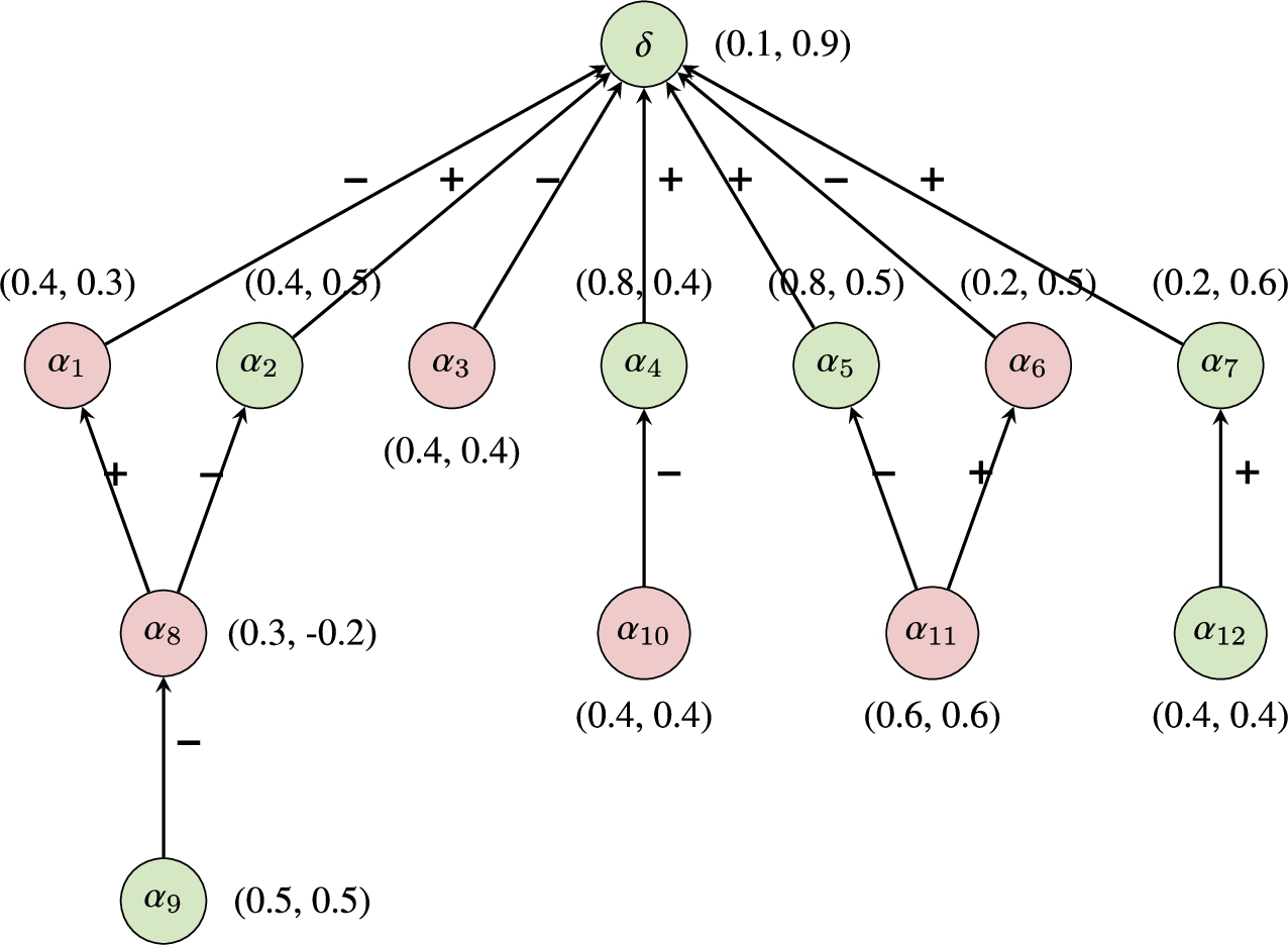
Example of QBAFc used as a counterexample in Appendix A.5. With each argument, there is a value pair (x,y) where x and y represent the base score and the strength (based on the logistic regression semantics σ) of the argument, respectively. The color represents the argument’s supported class (i.e., green for positive (1) and red for negative (0)).

Fig. 15.

The corresponding QBAFc′ of the QBAFc in Fig. 14, used as a counterexample in Appendix A.5. With each argument, there is a value pair (x,y) where x and y represent the base score and the strength (based on the logistic regression semantics σ) of the argument, respectively. The color represents the argument’s supported class (i.e., green for positive (1) and red for negative (0)).

Proposition 1.

Both ⟨QBAFc,σ⟩ and ⟨QBAFc′,σ⟩ satisfy GP1.

Proof.

According to Definition 3, with R−(α)=∅ and R+(α)=∅, we have σ(α)=τ(α)+∑b∈∅σ(b)ν(b)−∑b∈∅σ(b)ν(b)=τ(α) as required.

Hence, both ⟨QBAFc,σ⟩ and ⟨QBAFc′,σ⟩ satisfy GP1. □

Proposition 2.

⟨QBAFc,σ⟩ does not satisfy GP2, but ⟨QBAFc′,σ⟩ does.

Proof.

According to Definition 3, with R+(α)=∅, we have

σ(α)=τ(α)+∑b∈∅σ(b)ν(b)−∑b∈R−(α)σ(b)ν(b)=τ(α)−∑b∈R−(α)σ(b)ν(b).

In QBAFc, σ(b) could be either positive or negative, so it is possible that ∑b∈R−(α)σ(b)ν(b)<0, making σ(α)>τ(α). α2 in Fig. 14 is one counterexample of this GP. By contrast, in QBAFc′, we have removed any attacker and supporter of which the strength is zero. According to this and Corollary 1, σ(b)>0 for b∈R−(α). Therefore, ∑b∈R−(α)σ(b)ν(b)>0, resulting in σ(α)<τ(α) as required.

Hence, ⟨QBAFc,σ⟩ does not satisfy GP2, but ⟨QBAFc′,σ⟩ does. □

Proposition 3.

⟨QBAFc,σ⟩ does not satisfy GP3, but ⟨QBAFc′,σ⟩ does.

Proof.

According to Definition 3, with R−(α)=∅, we have

σ(α)=τ(α)+∑b∈R+(α)σ(b)ν(b)−∑b∈∅σ(b)ν(b)=τ(α)+∑b∈R+(α)σ(b)ν(b).

As in the proof of GP2, for QBAFc, ∑b∈R+(α)σ(b)ν(b) could be negative, rendering σ(α)<τ(α). α1 in Fig. 14 is one counterexample of this GP. Meanwhile, in QBAFc′, ∑b∈R+(α)σ(b)ν(b)>0. Therefore, σ(α)>τ(α) as required.

Hence, ⟨QBAFc,σ⟩ does not satisfy GP3, but ⟨QBAFc′,σ⟩ does. □

Proposition 4.

⟨QBAFc,σ⟩ does not satisfy GP4, but ⟨QBAFc′,σ⟩ does.

Proof.

From σ(α)<τ(α) with Definition 3, we obtain that

σ(α)=τ(α)+∑b∈R+(α)σ(b)ν(b)−∑b∈R−(α)σ(b)ν(b)<τ(α).

Therefore,

∑b∈R+(α)σ(b)ν(b)−∑b∈R−(α)σ(b)ν(b)<0.

For QBAFc, it is possible that R−(α)=∅ because ∑b∈R+(α)σ(b)ν(b) could be negative, satisfying the inequality. So, the property is not satisfied. α1 in Fig. 14 is one counterexample of this GP. In contrast, for QBAFc′, let us proof by contradiction. Assume that R−(α)=∅. We will obtain ∑b∈R+(α)σ(b)ν(b)<0 which is impossible under QBAFc′ where σ(b)>0. Therefore, it must be the case that R−(α)≠∅.

Hence, ⟨QBAFc,σ⟩ does not satisfy GP4, but ⟨QBAFc′,σ⟩ does. □

Proposition 5.

⟨QBAFc,σ⟩ does not satisfy GP5, but ⟨QBAFc′,σ⟩ does.

Proof.

From σ(α)>τ(α) with Definition 3, we obtain that

σ(α)=τ(α)+∑b∈R+(α)σ(b)ν(b)−∑b∈R−(α)σ(b)ν(b)>τ(α).

Therefore,

∑b∈R+(α)σ(b)ν(b)−∑b∈R−(α)σ(b)ν(b)>0.

As in the proof of GP4, for QBAFc, it is possible that R+(α)=∅ because ∑b∈R−(α)σ(b)ν(b) could be negative, satisfying the inequality. So, the property is not satisfied. α2 in Fig. 14 is one counterexample of this GP. In contrast, for QBAFc′, let us proof by contradiction. Assume that R+(α)=∅. We will obtain −∑b∈R−(α)σ(b)ν(b)>0. Thus, ∑b∈R−(α)σ(b)ν(b)<0 which is impossible under QBAFc′ where σ(b)>0. Therefore, it must be the case that R+(α)≠∅.

Hence, ⟨QBAFc,σ⟩ does not satisfy GP5, but ⟨QBAFc′,σ⟩ does. □

Proposition 6.

Both ⟨QBAFc,σ⟩ and ⟨QBAFc′,σ⟩ satisfy GP6.

Proof.

According to Definition 3, we have

σ(α)=τ(α)+∑b∈R+(α)σ(b)ν(b)−∑b∈R−(α)σ(b)ν(b).

Because R−(α)=R−(β), R+(α)=R+(β), and τ(α)=τ(β), we can replace τ(α), R+(α), and R−(α) by τ(β), R+(β), and R−(β), respectively. Therefore,

σ(α)=τ(β)+∑b∈R+(β)σ(b)ν(b)−∑b∈R−(β)σ(b)ν(b)=σ(β).

Hence, both ⟨QBAFc,σ⟩ and ⟨QBAFc′,σ⟩ satisfy GP6. □

Proposition 7.

⟨QBAFc,σ⟩ does not satisfy GP7, but ⟨QBAFc′,σ⟩ does.

Proof.

Since R−(α)⊂R−(β), we can partition R−(β) into two disjoint sets which are R−(α) and a non-empty set of arguments X=R−(β)−R−(α). According to Definition 3, we have

σ(β)=τ(β)+∑b∈R+(β)σ(b)ν(b)−∑b∈R−(β)σ(b)ν(b)=τ(β)+∑b∈R+(β)σ(b)ν(b)−∑b∈R−(α)σ(b)ν(b)−∑b∈Xσ(b)ν(b)

Because R+(α)=R+(β) and τ(α)=τ(β), we obtain that

σ(β)=τ(α)+∑b∈R+(α)σ(b)ν(b)−∑b∈R−(α)σ(b)ν(b)−∑b∈Xσ(b)ν(b)=σ(α)−∑b∈Xσ(b)ν(b)

As in the previous proofs, for QBAFc, it is possible that ∑b∈Xσ(b)ν(b)<0, rendering σ(α)<σ(β) and unsatisfying GP7. We can find a counterexample in Fig. 14 with α=α3 and β=α2. In contrast, for QBAFc′, σ(b)>0. Therefore, ∑b∈Xσ(b)ν(b) is always greater than 0. As a result, σ(α)>σ(β) as required.

Hence, ⟨QBAFc,σ⟩ does not satisfy GP7, but ⟨QBAFc′,σ⟩ does. □

Proposition 8.

⟨QBAFc,σ⟩ does not satisfy GP8, but ⟨QBAFc′,σ⟩ does.

Proof.

Since R+(α)⊂R+(β), we can partition R+(β) into two disjoint sets which are R+(α) and a non-empty set of arguments X=R+(β)−R+(α). According to Definition 3, we have

σ(β)=τ(β)+∑b∈R+(β)σ(b)ν(b)−∑b∈R−(β)σ(b)ν(b)=τ(β)+∑b∈R+(α)σ(b)ν(b)+∑b∈Xσ(b)ν(b)−∑b∈R−(β)σ(b)ν(b)

Because R−(α)=R−(β) and τ(α)=τ(β), we obtain that

σ(β)=τ(α)+∑b∈R+(α)σ(b)ν(b)−∑b∈R−(α)σ(b)ν(b)+∑b∈Xσ(b)ν(b)=σ(α)+∑b∈Xσ(b)ν(b)

As in the previous proofs, for QBAFc, it is possible that ∑b∈Xσ(b)ν(b)<0, rendering σ(α)>σ(β) and unsatisfying GP8. We can find a counterexample in Fig. 14 with α=α3 and β=α1. In contrast, for QBAFc′, σ(b)>0. Therefore, ∑b∈Xσ(b)ν(b) is always greater than 0. As a result, σ(α)<σ(β) as required.

Hence, ⟨QBAFc,σ⟩ does not satisfy GP8, but ⟨QBAFc′,σ⟩ does. □

Proposition 9.

Both ⟨QBAFc,σ⟩ and ⟨QBAFc′,σ⟩ satisfy GP9.

Proof.

Let us proof by contradiction. Assume that σ(α)⩾σ(β). Applying Definition 3, we obtain

τ(α)+∑b∈R+(α)σ(b)ν(b)−∑b∈R−(α)σ(b)ν(b)⩾τ(β)+∑b∈R+(β)σ(b)ν(b)−∑b∈R−(β)σ(b)ν(b)

Because R−(α)=R−(β) and R+(α)=R+(β),

τ(α)+∑b∈R+(α)σ(b)ν(b)−∑b∈R−(α)σ(b)ν(b)⩾τ(β)+∑b∈R+(α)σ(b)ν(b)−∑b∈R−(α)σ(b)ν(b)τ(α)⩾τ(β)

However, this contradicts the given statement that τ(α)<τ(β), so σ(α)⩾σ(β) cannot be true. Thus, σ(α)<σ(β) as required.

Hence, both ⟨QBAFc,σ⟩ and ⟨QBAFc′,σ⟩ satisfy GP9. □

Note again that the definition of < between two sets used in GP10 and GP11 is defined as follows. Given P and Q are subsets of A, P⩽Q if and only if there exists an injective mapping f from P to Q such that ∀α∈P, σ(α)⩽σ(f(α)). Furthermore, P<Q if and only if P⩽Q but Q≰P.

Proposition 10.

Both ⟨QBAFc,σ⟩ and ⟨QBAFc′,σ⟩ do not satisfy GP10.

Proof.

Counterexamples of this GP for QBAFc and QBAFc′ are in Figs 14 and 15, respectively, where α=α4 and β=α5. We can see that R−(α)⩽R−(β) as we have a mapping from R−(α) to R−(β), f={(α10,α11)}, where ∀a∈R−(α), σ(a)⩽σ(f(a)). In this case, σ(α10)⩽σ(α11). However, R−(β)≰R−(α). So, R−(α)<R−(β). In addition, R+(α)=R+(β)=∅ and τ(α)=τ(β)=0.4. Nevertheless, σ(α)=0.4 and σ(β)=0.5, so σ(α)>σ(β) is not true.

Hence, both ⟨QBAFc,σ⟩ and ⟨QBAFc′,σ⟩ do not satisfy GP10. (This is because σ considers not only the strengths of the attackers and the supporters but also their out-degrees.) □

Proposition 11.

Both ⟨QBAFc,σ⟩ and ⟨QBAFc′,σ⟩ do not satisfy GP11.

Proof.

Counterexamples of this GP for QBAFc and QBAFc′ are in Figs 14 and 15, respectively, where α=α7 and β=α6. We can see that R+(α)⩽R+(β) as we have a mapping from R+(α) to R+(β), f={(α12,α11)}, where ∀a∈R+(α), σ(a)⩽σ(f(a)). In this case, σ(α12)⩽σ(α11). However, R+(β)≰R+(α). So, R+(α)<R+(β). In addition, R−(α)=R−(β)=∅ and τ(α)=τ(β)=0.2. Nevertheless, σ(α)=0.6 and σ(β)=0.5, so σ(α)<σ(β) is not true.

Hence, both ⟨QBAFc,σ⟩ and ⟨QBAFc′,σ⟩ do not satisfy GP11. (This is because σ considers not only the strengths of the attackers and the supporters but also their out-degrees.) □

Appendix B.

Appendix B.Machine learning terminology

This section explains meanings of technical terms concerning machine learning and classification that are used in this paper.

Dataset splits. Working on a classification task, we usually divide a dataset we have into three splits. The first split is a training set, which is used to train our classification model. The second split is a test set, which is used to evaluate the final trained model. The third split is a development set (also called a validation set), which is used to evaluate model(s) under development so as to choose the best model architecture or hyperparameters. To ensure that the model can generalize beyond what it sees during training and development, all the three data splits must be mutually exclusive.

Because logistic regression (LR) does not have any hyperparameters or multiple architectures to choose, we did not use the development set while training the LR models in our experiments (Sections 7–10). However, in Section 10, we used the development set of the deceptive hotel review dataset for two purposes – (i) to tune the regularization hyperparameter of the support vector machine (SVM) model and (ii) to generate explanations for tutoring human participants to detect deceptive reviews.

Evaluation metrics. For binary classification, let y and yˆ be the true class and the predicted class of an example x, respectively. Hence, both y and yˆ could be either 0 or 1, resulting in four possible situations.

True Positive (TP): The model correctly predicts that the class of x is 1 (i.e., y=yˆ=1).
True Negative (TN): The model correctly predicts that the class of x is 0 (i.e., y=yˆ=0).
False Positive (FP): The model predicts that the class of x is 1 (i.e., yˆ=1), but the true class of x is in fact 0 (i.e., y=0).
False Negative (TN): The model predicts that the class of x is 0 (i.e., yˆ=0), but the true class of x is in fact 1 (i.e., y=1).

By default, we consider class 1 to be the positive class and consider class 0 to be the negative class. However, we can also consider the four situations above with respect to a specific class c. Particularly, TPc (true positives) and FPc (false positives) are the number of examples predicted as class c by the classifier that are correct and incorrect predictions, respectively. FNc (false negatives) is the number of examples with class c as their true label but the model does not predict correctly. TNc (true negatives) is the number of examples where the true label is not class c and the model also does not predict class c.

To evaluate the performance of a classifier, we apply it to predict examples in a labeled test dataset D′ and report the percentage of correct predictions, so called the accuracy or classification rate.

(9)Accuracy=|{(xi,yi)∈D′|yˆi=yi}||D′|=TP+TNTP+TN+FP+FN

However, if the test dataset is class imbalanced, i.e., having examples of one class more than the other, accuracy may not be the best evaluation metric because a model can get a high accuracy only by always answering the majority class. Alternatively, we can report the model performance for each specific class c∈{0,1} using the class precision, recall, and F1, defined as follows [29, chapter 4].

(10)Precisionc=Pc=TPcTPc+FPc=|{(xi,yi)∈D′|yˆi=yi=c}||{(xi,yi)∈D′|yˆi=c}|(11)Recallc=Rc=TPcTPc+FNc=|{(xi,yi)∈D′|yˆi=yi=c}||{(xi,yi)∈D′|yi=c}|(12)F1c=2PcRcPc+Rc

There are two ways to aggregate the class-specific metrics to be the metrics for the overall performance. First, micro-averaging combines the TP, FP, and FN of all classes (in C) before computing precision and recall.

(13)Micro Precision=∑c∈CTPc∑c∈CTPc+∑c∈CFPc(14)Micro Recall=∑c∈CTPc∑c∈CTPc+∑c∈CFNc(15)Micro F1=2×Micro Precision×Micro RecallMicro Precision+Micro Recall

Second, macro-averaging averages out precision and recall scores of all the classes so all the classes are weighted equally regardless of their size.

(16)Macro Precision=1|C|∑c∈CPc(17)Macro Recall=1|C|∑c∈CRc(18)Macro F1=2×Macro Precision×Macro RecallMacro Precision+Macro Recall

Normally, when we work with datasets that are class imbalanced, we want the model to work well for all the classes, not just for the majority class. Therefore, we often use macro F1 as the main evaluation metric in addition to the classification accuracy.

Appendix C.

Appendix C.Additional results of Section 8.1 – statistics for QBAFcs and QBAFc′s

Along with the results in Section 8.1, we additionally present the statistics for QBAFcs (before the post-processing step) compared to QBAFc′s (after the post-processing step) here. Tables 14–16 show the statistics for the SMS Spam Collection, Amazon Clothes, and Deceptive Hotel Reviews datasets, respectively. In addition to the number of arguments, we measure the number of pairs in the (attacks and support) relations (i.e., R=R−∪R+), and specifically those not involving the default argument (i.e., R∖δ={(a,b)∈R|b≠δ}). Note that, if R∖δ=∅, then the generated AXPLR amounts to a FLX where we do not consider relationships between features. We further discussed interesting aspects of the statistics below.

Table 14

Statistics (Average ± SD) of QBAFc and QBAFc′ for the SMS Spam Collection dataset. TP, TN, FP, and FN stand for true positives, true negatives, false positives, and false negatives, respectively. A+,δ, A−,δ are sets of arguments supporting positive and negative classes, respectively. R is a set of (attack and support) relations, whereas R∖δ is a subset of R containing specifically those not involving the default argument δ

Measurement	TQBAFc	TQBAFc′	BQBAFc	BQBAFc′
# Examples	1115 (TP: 115, TN: 972, FP: 5, FN: 23)
\|A\|	10.08 ± 11.55	10.08 ± 11.55	10.08 ± 11.55	10.08 ± 11.55
– TP	35.98 ± 12.26	35.98 ± 12.26	35.98 ± 12.26	35.98 ± 12.26
– TN	6.66 ± 6.01	6.66 ± 6.01	6.66 ± 6.01	6.66 ± 6.01
– FP	36.00 ± 11.98	36.00 ± 11.98	36.00 ± 11.98	36.00 ± 11.98
– FN	19.30 ± 9.66	19.30 ± 9.66	19.30 ± 9.66	19.30 ± 9.66
\|A+,δ\|	5.86 ± 7.12	6.25 ± 7.77	5.86 ± 7.12	6.47 ± 8.07
– TP	22.36 ± 7.17	24.68 ± 7.70	22.36 ± 7.17	25.42 ± 7.52
– TN	3.70 ± 3.57	3.85 ± 3.69	3.70 ± 3.57	4.00 ± 4.01
– FP	20.40 ± 6.31	22.20 ± 6.87	20.40 ± 6.31	24.20 ± 6.02
– FN	11.26 ± 4.73	11.74 ± 4.83	11.26 ± 4.73	12.48 ± 5.69
\|A−,δ\|	4.22 ± 4.63	3.83 ± 4.14	4.22 ± 4.63	3.61 ± 3.81
– TP	13.63 ± 5.60	11.30 ± 5.37	13.63 ± 5.60	10.57 ± 5.41
– TN	2.96 ± 2.66	2.81 ± 2.65	2.96 ± 2.66	2.66 ± 2.33
– FP	15.60 ± 5.77	13.80 ± 5.50	15.60 ± 5.77	11.80 ± 6.06
– FN	8.04 ± 5.17	7.57 ± 5.29	8.04 ± 5.17	6.83 ± 4.25
\|R\|	11.64 ± 16.77	11.64 ± 16.77	13.82 ± 21.40	13.82 ± 21.40
– TP	49.31 ± 19.63	49.31 ± 19.63	61.43 ± 26.11	61.43 ± 26.11
– TN	6.69 ± 8.17	6.69 ± 8.17	7.57 ± 10.37	7.57 ± 10.37
– FP	50.60 ± 21.14	50.60 ± 21.14	64.20 ± 28.35	64.20 ± 28.35
– FN	23.96 ± 14.27	23.96 ± 14.27	29.17 ± 19.09	29.17 ± 19.09
\|R∖δ\|	8.32 ± 14.76	8.32 ± 14.76	8.32 ± 14.76	8.32 ± 14.76
– TP	40.81 ± 18.81	40.81 ± 18.81	40.81 ± 18.81	40.81 ± 18.81
– TN	4.06 ± 7.09	4.06 ± 7.09	4.06 ± 7.09	4.06 ± 7.09
– FP	43.40 ± 21.41	43.40 ± 21.41	43.40 ± 21.41	43.40 ± 21.41
– FN	18.43 ± 13.93	18.43 ± 13.93	18.43 ± 13.93	18.43 ± 13.93
\|R−\|	6.39 ± 8.48	5.31 ± 6.33	7.51 ± 10.90	5.73 ± 7.93
– TP	24.92 ± 9.91	16.50 ± 8.10	31.50 ± 13.48	20.22 ± 11.75
– TN	3.95 ± 4.43	3.74 ± 4.15	4.36 ± 5.43	3.75 ± 4.71
– FP	26.60 ± 10.83	20.60 ± 10.36	32.40 ± 14.84	22.40 ± 12.95
– FN	12.78 ± 7.11	12.13 ± 6.59	15.30 ± 9.18	13.35 ± 7.79
\|R+\|	5.24 ± 8.49	6.33 ± 10.88	6.31 ± 10.72	8.10 ± 13.88
– TP	24.39 ± 10.38	32.81 ± 12.21	29.93 ± 13.40	41.22 ± 15.19
– TN	2.74 ± 3.99	2.95 ± 4.28	3.21 ± 5.20	3.82 ± 5.85
– FP	24.00 ± 10.89	30.00 ± 11.07	31.80 ± 14.04	41.80 ± 15.69
– FN	11.17 ± 7.51	11.83 ± 7.95	13.87 ± 10.33	15.83 ± 11.62

Table 15

Statistics (Average ± SD) of QBAFc and QBAFc′ for the Amazon Clothes dataset. TP, TN, FP, and FN stand for true positives, true negatives, false positives, and false negatives, respectively. A+,δ, A−,δ are sets of arguments supporting positive and negative classes, respectively. R is a set of (attack and support) relations, whereas R∖δ is a subset of R containing specifically those not involving the default argument δ

Measurement	TQBAFc	TQBAFc′	BQBAFc	BQBAFc′
# Examples	10000 (TP: 4176, TN: 4186, FP: 848, FN: 790)
\|A\|	16.09 ± 8.13	16.09 ± 8.13	16.09 ± 8.13	16.09 ± 8.13
– TP	14.85 ± 7.57	14.85 ± 7.57	14.85 ± 7.57	14.85 ± 7.57
– TN	17.45 ± 8.21	17.45 ± 8.21	17.45 ± 8.21	17.45 ± 8.21
– FP	14.99 ± 8.14	14.99 ± 8.14	14.99 ± 8.14	14.99 ± 8.14
– FN	16.57 ± 9.31	16.57 ± 9.31	16.57 ± 9.31	16.57 ± 9.31
\|A+,δ\|	7.39 ± 4.36	7.45 ± 4.50	7.39 ± 4.36	7.43 ± 4.88
– TP	8.91 ± 4.18	9.74 ± 4.07	8.91 ± 4.18	10.22 ± 4.51
– TN	5.93 ± 3.98	5.20 ± 3.76	5.93 ± 3.98	4.75 ± 3.68
– FP	7.80 ± 4.27	8.47 ± 4.12	7.80 ± 4.27	8.49 ± 4.34
– FN	6.65 ± 4.55	6.10 ± 4.29	6.65 ± 4.55	5.84 ± 4.37
\|A−,δ\|	8.70 ± 5.23	8.64 ± 5.89	8.70 ± 5.23	8.65 ± 6.24
– TP	5.94 ± 3.99	5.10 ± 4.18	5.94 ± 3.99	4.63 ± 4.27
– TN	11.52 ± 4.96	12.25 ± 5.36	11.52 ± 4.96	12.71 ± 5.53
– FP	7.19 ± 4.18	6.52 ± 4.38	7.19 ± 4.18	6.50 ± 4.44
– FN	9.92 ± 5.14	10.47 ± 5.49	9.92 ± 5.14	10.73 ± 5.57
\|R\|	17.64 ± 10.25	17.64 ± 10.25	21.68 ± 13.29	21.68 ± 13.29
– TP	16.33 ± 9.78	16.33 ± 9.78	20.55 ± 12.49	20.55 ± 12.49
– TN	19.10 ± 10.20	19.10 ± 10.20	23.07 ± 13.47	23.07 ± 13.47
– FP	16.38 ± 10.47	16.38 ± 10.47	20.06 ± 13.57	20.06 ± 13.57
– FN	18.18 ± 11.57	18.18 ± 11.57	22.03 ± 15.32	22.03 ± 15.32
\|R∖δ\|	12.71 ± 8.73	12.71 ± 8.73	12.71 ± 8.73	12.71 ± 8.73
– TP	12.34 ± 8.42	12.34 ± 8.42	12.34 ± 8.42	12.34 ± 8.42
– TN	13.30 ± 8.74	13.30 ± 8.74	13.30 ± 8.74	13.30 ± 8.74
– FP	11.68 ± 9.01	11.68 ± 9.01	11.68 ± 9.01	11.68 ± 9.01
– FN	12.65 ± 9.77	12.65 ± 9.77	12.65 ± 9.77	12.65 ± 9.77
\|R−\|	5.27 ± 3.79	5.11 ± 3.96	8.10 ± 5.54	4.08 ± 3.47
– TP	4.74 ± 3.55	5.50 ± 4.38	8.20 ± 5.18	3.72 ± 3.43
– TN	5.73 ± 3.86	4.56 ± 3.27	8.00 ± 5.70	4.12 ± 3.31
– FP	5.20 ± 3.82	6.30 ± 4.66	8.09 ± 5.73	5.15 ± 3.75
– FN	5.61 ± 4.25	4.68 ± 3.67	8.14 ± 6.31	4.72 ± 3.84
\|R+\|	12.38 ± 7.04	12.53 ± 7.20	13.58 ± 8.44	17.59 ± 10.52
– TP	11.59 ± 6.76	10.83 ± 5.97	12.35 ± 7.72	16.83 ± 9.79
– TN	13.37 ± 6.98	14.54 ± 7.64	15.06 ± 8.65	18.95 ± 10.82
– FP	11.18 ± 7.16	10.08 ± 6.30	11.97 ± 8.35	14.91 ± 10.26
– FN	12.56 ± 7.92	13.49 ± 8.52	13.89 ± 9.65	17.32 ± 11.89

Table 16

Statistics (Average ± SD) of QBAFc and QBAFc′ for the Deceptive Hotel Review dataset. TP, TN, FP, and FN stand for true positives, true negatives, false positives, and false negatives, respectively. A+,δ, A−,δ are sets of arguments supporting positive and negative classes, respectively. R is a set of (attack and support) relations, whereas R∖δ is a subset of R containing specifically those not involving the default argument δ

Measurement	TQBAFc	TQBAFc′	BQBAFc	BQBAFc′
# Examples	320 (TP: 130, TN: 143, FP: 26, FN: 21)
\|A\|	19.44 ± 6.82	19.44 ± 6.82	19.44 ± 6.82	19.44 ± 6.82
– TP	19.54 ± 6.54	19.54 ± 6.54	19.54 ± 6.54	19.54 ± 6.54
– TN	20.24 ± 6.86	20.24 ± 6.86	20.24 ± 6.86	20.24 ± 6.86
– FP	17.77 ± 6.48	17.77 ± 6.48	17.77 ± 6.48	17.77 ± 6.48
– FN	15.48 ± 7.34	15.48 ± 7.34	15.48 ± 7.34	15.48 ± 7.34
\|A+,δ\|	9.14 ± 4.46	9.89 ± 5.02	9.14 ± 4.46	10.34 ± 5.00
– TP	12.06 ± 4.27	13.58 ± 4.53	12.06 ± 4.27	13.85 ± 4.50
– TN	6.85 ± 3.11	6.92 ± 3.21	6.85 ± 3.11	7.43 ± 3.32
– FP	9.50 ± 3.56	10.77 ± 3.74	9.50 ± 3.56	11.42 ± 4.09
– FN	6.19 ± 3.60	6.29 ± 3.61	6.19 ± 3.60	7.10 ± 3.96
\|A−,δ\|	10.30 ± 4.91	9.55 ± 5.33	10.30 ± 4.91	9.10 ± 5.13
– TP	7.48 ± 3.16	5.96 ± 3.14	7.48 ± 3.16	5.69 ± 2.93
– TN	13.39 ± 4.77	13.32 ± 4.81	13.39 ± 4.77	12.81 ± 4.68
– FP	8.27 ± 3.34	7.00 ± 3.27	8.27 ± 3.34	6.35 ± 2.86
– FN	9.29 ± 4.23	9.19 ± 4.19	9.29 ± 4.23	8.38 ± 3.77
\|R\|	22.03 ± 9.43	22.03 ± 9.43	21.48 ± 9.62	21.48 ± 9.62
– TP	23.96 ± 9.93	23.96 ± 9.93	23.12 ± 10.32	23.12 ± 10.32
– TN	21.41 ± 8.69	21.41 ± 8.69	21.01 ± 8.67	21.01 ± 8.67
– FP	20.04 ± 8.88	20.04 ± 8.88	20.00 ± 9.75	20.00 ± 9.75
– FN	16.81 ± 9.35	16.81 ± 9.35	16.29 ± 9.37	16.29 ± 9.37
\|R∖δ\|	8.19 ± 6.35	8.19 ± 6.35	8.19 ± 6.35	8.19 ± 6.35
– TP	10.69 ± 7.09	10.69 ± 7.09	10.69 ± 7.09	10.69 ± 7.09
– TN	6.47 ± 5.13	6.47 ± 5.13	6.47 ± 5.13	6.47 ± 5.13
– FP	7.35 ± 5.64	7.35 ± 5.64	7.35 ± 5.64	7.35 ± 5.64
– FN	5.52 ± 4.59	5.52 ± 4.59	5.52 ± 4.59	5.52 ± 4.59
\|R−\|	9.30 ± 4.35	7.00 ± 3.43	8.43 ± 4.25	6.13 ± 3.24
– TP	11.41 ± 4.43	6.45 ± 3.34	10.43 ± 4.50	5.98 ± 3.51
– TN	7.75 ± 3.48	7.55 ± 3.34	6.96 ± 3.29	6.32 ± 2.96
– FP	9.58 ± 4.03	7.12 ± 3.84	8.81 ± 4.04	6.38 ± 3.65
– FN	6.52 ± 3.75	6.52 ± 3.75	5.52 ± 3.14	5.48 ± 2.91
\|R+\|	12.73 ± 6.18	15.03 ± 7.09	13.05 ± 6.45	15.34 ± 7.35
– TP	12.55 ± 6.27	17.52 ± 7.66	12.69 ± 6.54	17.14 ± 7.66
– TN	13.66 ± 6.03	13.86 ± 6.11	14.06 ± 6.25	14.69 ± 6.81
– FP	10.46 ± 5.58	12.92 ± 5.59	11.19 ± 6.15	13.62 ± 6.66
– FN	10.29 ± 6.29	10.29 ± 6.29	10.76 ± 6.74	10.81 ± 7.10

Number of relations. |R| had the similar trend as the number of arguments discussed in Section 8.1. Texts predicted as spams had a significantly higher number of attacks and supports than those predicted as non-spams (see |R−| and |R+| in Table 14). For the other two datasets, they usually had more supports than attacks, especially after post-processing, to provide sufficient evidence for the predictions. In any case, all three datasets had |R∖δ| from 8 to 12, on average, making the explanations extracted from the QBAFc′s (i.e., the AXPLR) different from the standard explanations for logistic regressions (i.e., the FLXs) due to many relations between features.

Other remarks. First, the number of arguments |A| for the TQBAFc, TQBAFc′, BQBAFc, and BQBAFc′ for the same example are always equal. This is expected from Definitions 2 and 4. Second, |R| is different for TQBAFcs and BQBAFcs but their |R∖δ| are the same. This is because TQBAFcs and BQBAFcs have the same relations between two non-default arguments except that the directions are reversed. For the relations with the default argument, TQBAFcs connect the arguments of the most general patterns to the default whereas BQBAFcs connect the most specific patterns to the default. That is why |R| was different between TQBAFcs and BQBAFcs. Lastly, post-processing does not change the number of pairs in relations in the experiments as shown by |R| of TQBAFcs and TQBAFc′s and |R| of BQBAFcs and BQBAFc′s. In theory, it could possibly change as the pairs (a,b) with σ(a)=0 are removed. However, because all the base scores in QBAFcs are from the weights of the trained LR model, each of which has around 15 decimal points, it is hardly possible to find an argument a with σ(a)=0 in practice. So, none of the pairs is removed during post-processing.

Appendix D.

Appendix D.Additional results of Section 8.2 – sufficiency

We also plot the sufficiency results for the three datasets in Figs 16–18. The x-axis of each plot is the number of supporting arguments used (k), whereas the y-axis shows the percentage of arguments (default or intermediate) of which the strength can be greater than 0 by using only k supporting arguments. Left subplots of these three figures are for the default arguments, whereas right subplots are for intermediate arguments. Class flipped means the supported class changes after post-processing (i.e., c′(δ)≠c(δ) for default arguments and c′(αi)≠c(αi) for intermediate arguments).

Fig. 16.

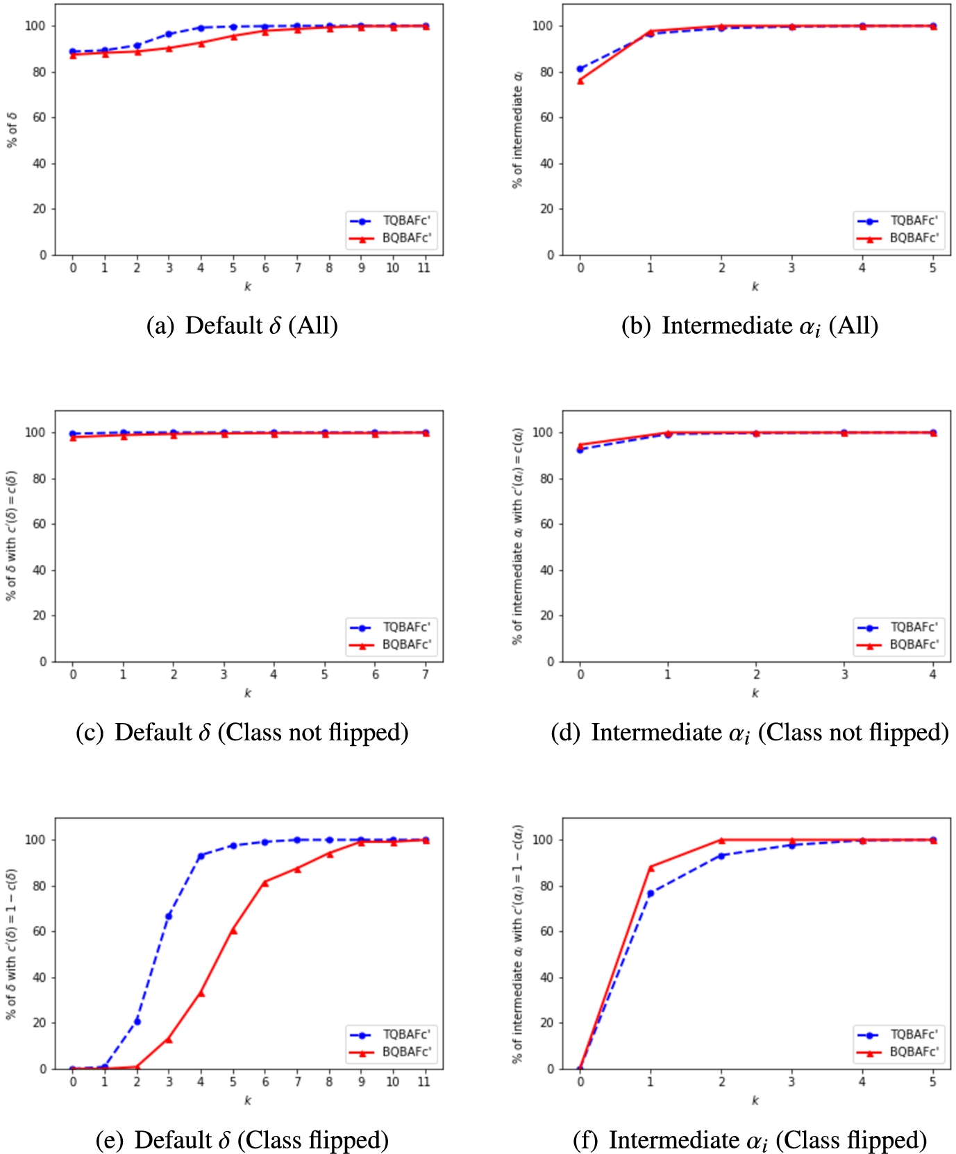
Plots showing the percentage of arguments (the default arguments δ or intermediate arguments αi) of which the strength can be greater than 0 using only k supporting arguments. These arguments are extracted from test examples of the SMS Spam Collection dataset. Class flipped means the supported class changes after post-processing.

Fig. 17.

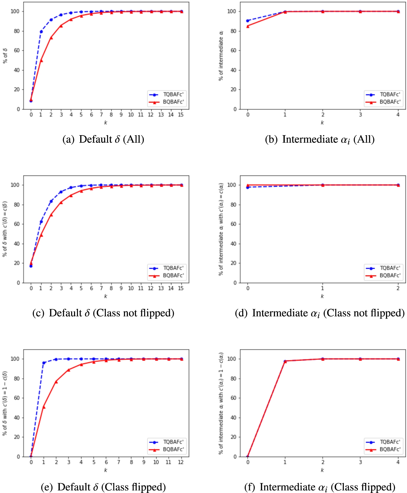
Plots showing the percentage of arguments (the default arguments δ or intermediate arguments αi) of which the strength can be greater than 0 using only k supporting arguments. These arguments are extracted from test examples of the Amazon Clothes dataset. Class flipped means the supported class changes after post-processing.

Fig. 18.

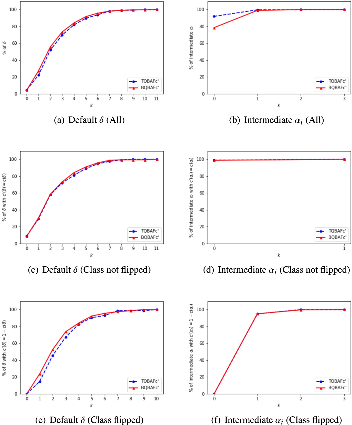
Plots showing the percentage of arguments (the default arguments δ or intermediate arguments αi) of which the strength can be greater than 0 using only k supporting arguments. These arguments are extracted from test examples of the Deceptive Hotel Reviews dataset. Class flipped means the supported class changes after post-processing.

Appendix E.

Appendix E.User interface for human participants in Experiment 2 (Section 9)

Figures 19 and 20 show some parts of the template used for rendering pattern questions in Experiment 2 for MTurk workers. This template is for the sentiment analysis task (i.e., the Amazon Clothes dataset). Additionally, Figs 21 and 22 are templates for rendering the group of sampled phrases and matched phrase questions of the same task, respectively. The user interface structures for the spam classification task were similar to the sentiment analysis task except that the five options of the spam task were Definitely Spam, Spam, Not sure, Non-spam, and Definitely Non-spam. For the full templates and additional details, please visit our GitHub repository – https://github.com/plkumjorn/AXPLR.

Fig. 19.

(First half) Some parts of the template used for rendering pattern questions from the sentiment analysis task (i.e., the Amazon Clothes dataset) for MTurk workers. It contains the instructions and a tutorial on how to read GrASP patterns.

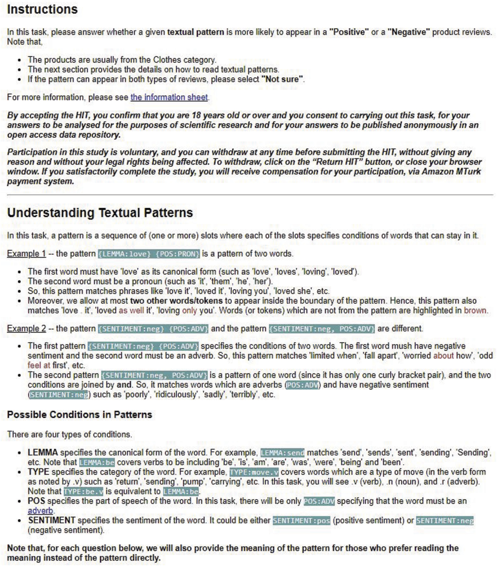
Fig. 20.

(Second half) Some parts of the template used for rendering pattern questions from the sentiment analysis task (i.e., the Amazon Clothes dataset) for MTurk workers. The actual interface contained 3 example questions and 10 actual questions. Each of the ${pattern_n} was substantiated by a GrASP pattern, while the ${translation_n} was substantiated by the corresponding meaning (i.e., textual description) of ${pattern_n}. Examples of substitutions of ${pattern_n} and ${translation_n} can be found in the above example questions.

$(Second half) Some parts of the template used for rendering pattern questions from the sentiment analysis task (i.e., the Amazon Clothes dataset) for MTurk workers. The actual interface contained 3 example questions and 10 actual questions. Each of the ${pattern_n} was substantiated by a GrASP pattern, while the ${translation_n} was substantiated by the corresponding meaning (i.e., textual description) of ${pattern_n}. Examples of substitutions of ${pattern_n} and ${translation_n} can be found in the above example questions.$

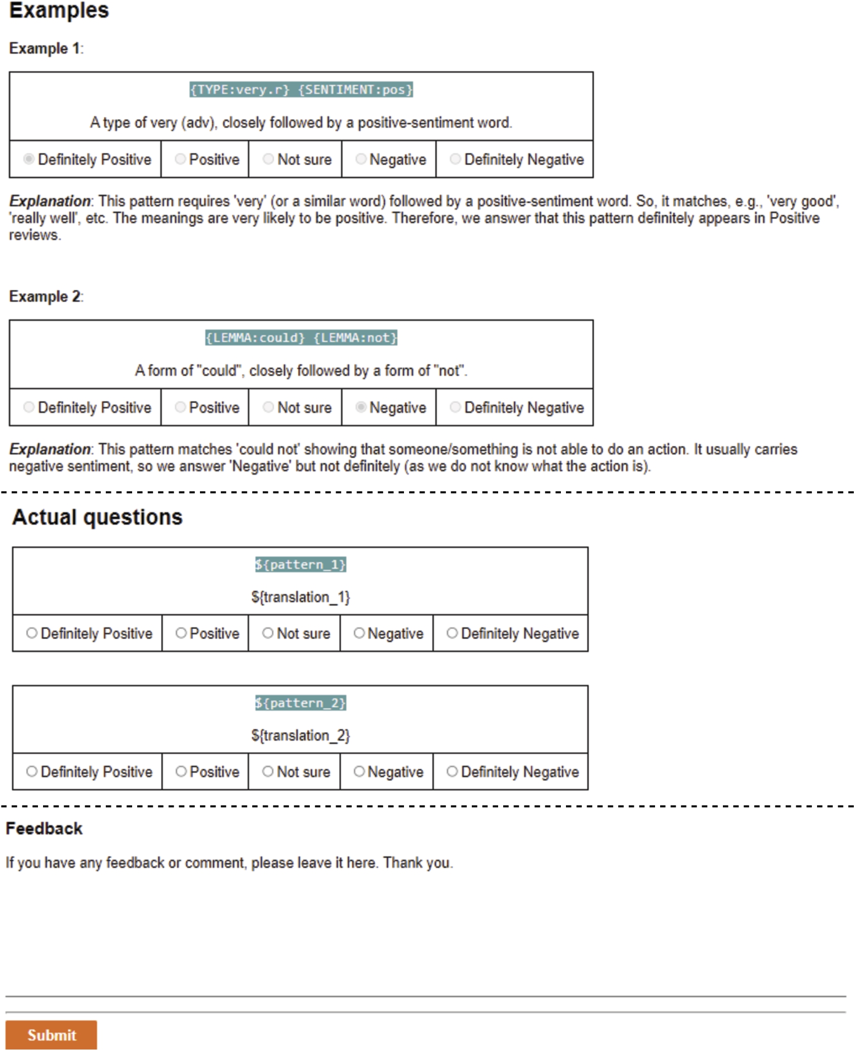
Fig. 21.

Some parts of the template used for rendering group of samples questions from the sentiment analysis task (i.e., the Amazon Clothes dataset) for MTurk workers. The actual interface contained 3 example questions and 10 actual questions. Each of the ${group_n} was substantiated by a group of sampled phrases for a specific pattern. An example of substitution of ${group_n} can be found in the above example question.

$Some parts of the template used for rendering group of samples questions from the sentiment analysis task (i.e., the Amazon Clothes dataset) for MTurk workers. The actual interface contained 3 example questions and 10 actual questions. Each of the ${group_n} was substantiated by a group of sampled phrases for a specific pattern. An example of substitution of ${group_n} can be found in the above example question.$

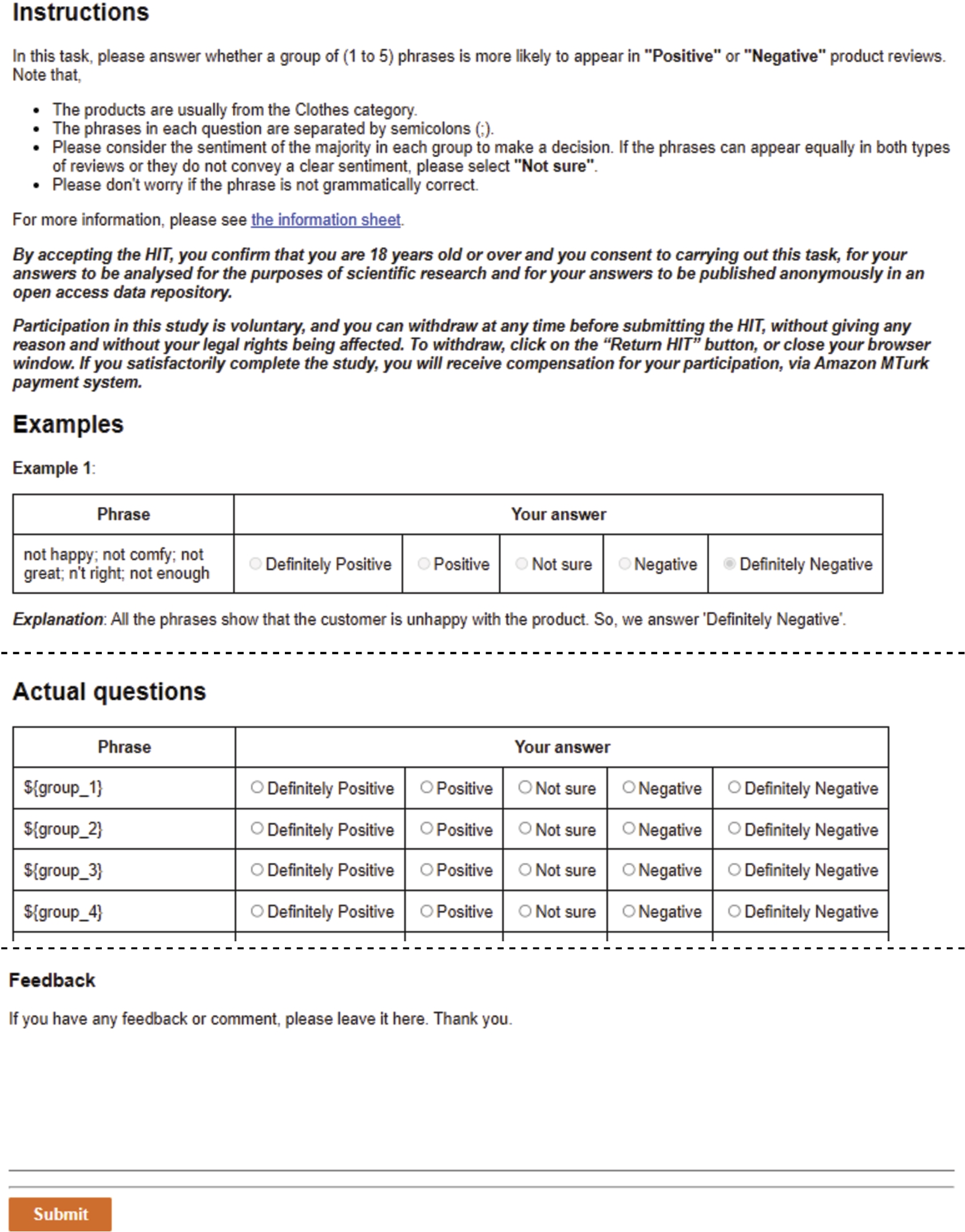
Fig. 22.

Some parts of the template used for rendering matched phrase questions from the sentiment analysis task (i.e., the Amazon Clothes dataset) for MTurk workers. The actual interface contained 3 example questions and 20 actual questions. Each of the ${phrase_n} was substantiated by an actual phrase. An example of substitution of ${phrase_n} can be found in the above example question.

$Some parts of the template used for rendering matched phrase questions from the sentiment analysis task (i.e., the Amazon Clothes dataset) for MTurk workers. The actual interface contained 3 example questions and 20 actual questions. Each of the ${phrase_n} was substantiated by an actual phrase. An example of substitution of ${phrase_n} can be found in the above example question.$

Appendix F.

Appendix F.User interface for human participants in Experiment 3 (Section 10)

Figure 23 shows an example post-test question with the actual Qualtrics survey user interface when there is no real-time assistance from any explanation method. In contrast, Figs 24–27 show the same post-test question but with real-time assistance from SVM, FLX, shallow AXPLR, and deep AXPLR, respectively. For other parts of the survey, please visit our GitHub repository – https://github.com/plkumjorn/AXPLR– to see how they were displayed to the participants.

Fig. 23.

Example of a post-test question without real-time assistance.

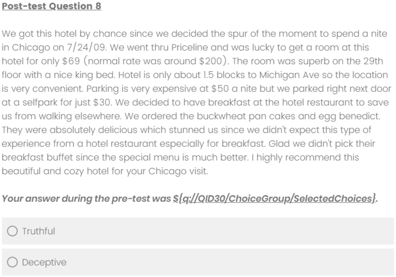
Fig. 24.

Example of a post-test question with real-time assistance using an SVM explanation.

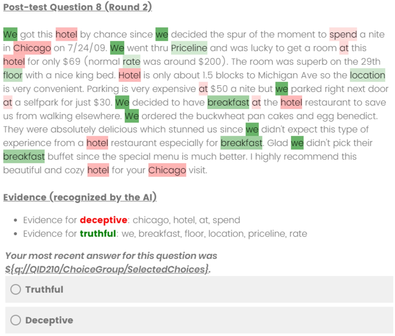
Fig. 25.

Example of a post-test question with real-time assistance using an FLX.

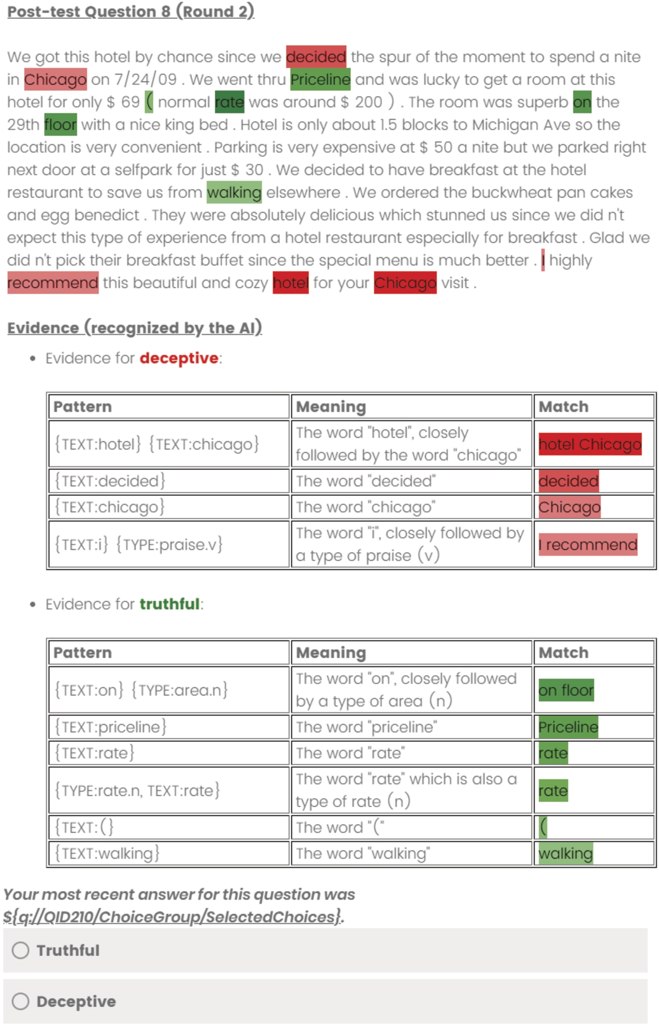
Fig. 26.

Example of a post-test question with real-time assistance using a shallow AXPLR.

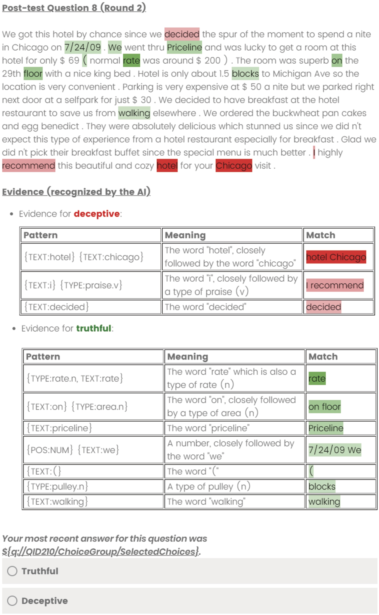
Fig. 27.

Example of a post-test question with real-time assistance using a deep AXPLR.

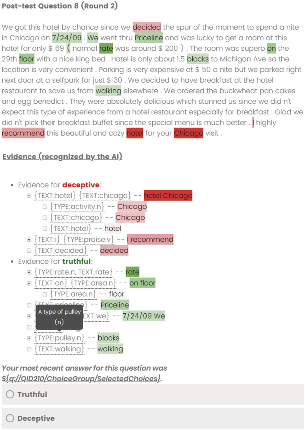
References

[1]	A. Adadi and M. Berrada, Peeking inside the black-box: A survey on explainable artificial intelligence (XAI), IEEE Access 6: ((2018) ), 52138–52160. doi:10.1109/ACCESS.2018.2870052.
[2]	E. Albini, P. Baroni, A. Rago and F. Toni, Interpreting and explaining pagerank through argumentation semantics, Intelligenza Artificiale 15: (1) ((2021) ), 17–34. doi:10.3233/IA-210095.
[3]	E. Albini, P. Lertvittayakumjorn, A. Rago and F. Toni, Dax: Deep argumentative explanation for neural networks, 2020, arXiv preprint arXiv:2012.05766.
[4]	E. Albini, A. Rago, P. Baroni and F. Toni, Influence-driven explanations for Bayesian network classifiers, in: Pacific Rim International Conference on Artificial Intelligence, Springer, (2021) , pp. 88–100.
[5]	T.A. Almeida, J.M.G. Hidalgo and A. Yamakami, Contributions to the study of SMS spam filtering: New collection and results, in: Proceedings of the 11th ACM Symposium on Document Engineering, (2011) , pp. 259–262. doi:10.1145/2034691.2034742.
[6]	L. Arras, F. Horn, G. Montavon, K.-R. Müller and W. Samek, Explaining predictions of non-linear classifiers in NLP, in: Proceedings of the 1st Workshop on Representation Learning for NLP, Association for Computational Linguistics, Berlin, Germany, (2016) , pp. 1–7, https://aclanthology.org/W16-1601. doi:10.18653/v1/W16-1601.
[7]	P. Baroni, A. Rago and F. Toni, From fine-grained properties to broad principles for gradual argumentation: A principled spectrum, International Journal of Approximate Reasoning 105: ((2019) ), 252–286. doi:10.1016/j.ijar.2018.11.019.
[8]	J. Brownlee, How to calculate feature importance with Python, 2020, Accessed: 2023-01-05.
[9]	L. Carstens and F. Toni, Using argumentation to improve classification in natural language problems, ACM Transactions on Internet Technology (TOIT) 17: (3) ((2017) ), 1–23. doi:10.1145/3017679.
[10]	R. Caruana, Y. Lou, J. Gehrke, P. Koch, M. Sturm and N. Elhadad, Intelligible models for healthcare: Predicting pneumonia risk and hospital 30-day readmission, in: Proceedings of the 21th ACM SIGKDD International Conference on Knowledge Discovery and Data Mining, (2015) , pp. 1721–1730. doi:10.1145/2783258.2788613.
[11]	O. Cocarascu, A. Rago and F. Toni, Extracting dialogical explanations for review aggregations with argumentative dialogical agents, in: Proceedings of the 18th International Conference on Autonomous Agents and MultiAgent Systems, Association for Computing Machinery, (2019) , pp. 1261–1269.
[12]	O. Cocarascu, A. Stylianou, K. Čyras and F. Toni, Data-empowered argumentation for dialectically explainable predictions, in: ECAI 2020, IOS Press, (2020) , pp. 2449–2456.
[13]	K. Čyras, D. Birch, Y. Guo, F. Toni, R. Dulay, S. Turvey, D. Greenberg and T. Hapuarachchi, Explanations by arbitrated argumentative dispute, Expert Systems with Applications 127: ((2019) ), 141–156. doi:10.1016/j.eswa.2019.03.012.
[14]	K. Čyras, A. Rago, E. Albini, P. Baroni and F. Toni, Argumentative XAI: A survey, 2021, arXiv preprint arXiv:2105.11266.
[15]	K. Čyras, K. Satoh and F. Toni, Explanation for case-based reasoning via abstract argumentation, in: Computational Models of Argument, IOS Press, (2016) , pp. 243–254.
[16]	A. Dejl, P. He, P. Mangal, H. Mohsin, B. Surdu, E. Voinea, E. Albini, P. Lertvittayakumjorn, A. Rago and F. Toni, Argflow: A toolkit for deep argumentative explanations for neural networks, in: Proceedings of the 20th International Conference on Autonomous Agents and MultiAgent Systems, International Foundation for Autonomous Agents and Multiagent Systems, Richland, SC, (2021) , pp. 1761–1763. ISBN 9781450383073.
[17]	J. Devlin, M.-W. Chang, K. Lee and K. Toutanova, BERT: Pre-training of deep bidirectional transformers for language understanding, in: Proceedings of the 2019 Conference of the North American Chapter of the Association for Computational Linguistics: Human Language Technologies, Volume 1 (Long and Short Papers), Association for Computational Linguistics, Minneapolis, Minnesota, (2019) , pp. 4171–4186, https://aclanthology.org/N19-1423. doi:10.18653/v1/N19-1423.
[18]	I.S. Efstathiadis, G. Paulino-Passos and F. Toni, Explainable patterns for distinction and prediction of moral judgement on Reddit, 2022, arXiv preprint arXiv:2201.11155.
[19]	J.L. Fleiss, Measuring nominal scale agreement among many raters, Psychological Bulletin 76: (5) ((1971) ), 378. doi:10.1037/h0031619.
[20]	M.M. Ghanem, Y. Guo, H. Lodhi and Y. Zhang, Automatic scientific text classification using local patterns: KDD Cup 2002 (task 1), ACM Sigkdd Explorations Newsletter 4: (2) ((2002) ), 95–96. doi:10.1145/772862.772876.
[21]	B. Goodman and S. Flaxman, European Union regulations on algorithmic decision-making and a “right to explanation”, AI Magazine 38: (3) ((2017) ), 50–57. doi:10.1609/aimag.v38i3.2741.
[22]	Y. Graham, N. Mathur and T. Baldwin, Randomized significance tests in machine translation, in: Proceedings of the Ninth Workshop on Statistical Machine Translation, Association for Computational Linguistics, Baltimore, Maryland, USA, (2014) , pp. 266–274, https://aclanthology.org/W14-3333. doi:10.3115/v1/W14-3333.
[23]	R. He and J. McAuley, Ups and downs: Modeling the visual evolution of fashion trends with one-class collaborative filtering, in: Proceedings of the 25th International Conference on World Wide Web, (2016) , pp. 507–517. doi:10.1145/2872427.2883037.
[24]	M. Hu and B. Liu, Mining and summarizing customer reviews, in: Proceedings of the Tenth ACM SIGKDD International Conference on Knowledge Discovery and Data Mining, (2004) , pp. 168–177. doi:10.1145/1014052.1014073.
[25]	M. Hussain, J. Hussain, T. Ali, S.I. Ali, H.S.M. Bilal, S. Lee and T. Chung, Text classification in clinical practice guidelines using machine-learning assisted pattern-based approach, Applied Sciences 11: (8) ((2021) ), 3296. doi:10.3390/app11083296.
[26]	A. Jacovi and Y. Goldberg, Towards faithfully interpretable NLP systems: How should we define and evaluate faithfulness? in: Proceedings of the 58th Annual Meeting of the Association for Computational Linguistics, Association for Computational Linguistics, Online, (2020) , pp. 4198–4205, https://aclanthology.org/2020.acl-main.386. doi:10.18653/v1/2020.acl-main.386.
[27]	A. Jacovi, A. Marasović, T. Miller and Y. Goldberg, Formalizing trust in artificial intelligence: Prerequisites, causes and goals of human trust in ai, in: Proceedings of the 2021 ACM Conference on Fairness, Accountability, and Transparency, (2021) , pp. 624–635. doi:10.1145/3442188.3445923.
[28]	S. Jain, S. Wiegreffe, Y. Pinter and B.C. Wallace, Learning to faithfully rationalize by construction, in: Proceedings of the 58th Annual Meeting of the Association for Computational Linguistics, Association for Computational Linguistics, Online, (2020) , pp. 4459–4473, https://aclanthology.org/2020.acl-main.409. doi:10.18653/v1/2020.acl-main.409.
[29]	D. Jurafsky and J.H. Martin, Speech & Language Processing, 3rd edn, (2020) , https://web.stanford.edu/~jurafsky/slp3/.
[30]	R. Khanna, B. Kim, J. Ghosh and S. Koyejo, Interpreting black box predictions using Fisher kernels, in: The 22nd International Conference on Artificial Intelligence and Statistics, PMLR, (2019) , pp. 3382–3390.
[31]	Y. Kim, Convolutional neural networks for sentence classification, in: Proceedings of the 2014 Conference on Empirical Methods in Natural Language Processing (EMNLP), Association for Computational Linguistics, Doha, Qatar, (2014) , pp. 1746–1751, https://aclanthology.org/D14-1181. doi:10.3115/v1/D14-1181.
[32]	P.W. Koh and P. Liang, Understanding black-box predictions via influence functions, in: International Conference on Machine Learning, PMLR, (2017) , pp. 1885–1894.
[33]	A. Krause and D. Golovin, Submodular function maximization, Tractability 3: ((2014) ), 71–104. doi:10.1017/CBO9781139177801.004.
[34]	V. Lai, H. Liu and C. Tan, “Why is ‘Chicago’ deceptive?” towards building model-driven tutorials for humans, in: Proceedings of the 2020 CHI Conference on Human Factors in Computing Systems, (2020) , pp. 1–13.
[35]	V. Lai and C. Tan, On human predictions with explanations and predictions of machine learning models: A case study on deception detection, in: Proceedings of the Conference on Fairness, Accountability, and Transparency, (2019) , pp. 29–38. doi:10.1145/3287560.3287590.
[36]	J. Lawrence and C. Reed, Argument mining: A survey, Computational Linguistics 45: (4) ((2020) ), 765–818. doi:10.1162/coli_a_00364.
[37]	T. Lei, R. Barzilay and T. Jaakkola, Rationalizing neural predictions, in: Proceedings of the 2016 Conference on Empirical Methods in Natural Language Processing, Association for Computational Linguistics, Austin, Texas, (2016) , pp. 107–117, https://aclanthology.org/D16-1011. doi:10.18653/v1/D16-1011.
[38]	P. Lertvittayakumjorn, L. Choshen, E. Shnarch and F. Toni, GrASP: A library for extracting and exploring human-interpretable textual patterns, 2021, arXiv preprint arXiv:2104.03958.
[39]	P. Lertvittayakumjorn, I. Petej, Y. Gao, Y. Krishnamurthy, A. Van Der Gaag, R. Jago and K. Stathis, Supporting complaints investigation for nursing and midwifery regulatory agencies, in: Proceedings of the 59th Annual Meeting of the Association for Computational Linguistics and the 11th International Joint Conference on Natural Language Processing: System Demonstrations, Association for Computational Linguistics, Online, (2021) , pp. 81–91, https://aclanthology.org/2021.acl-demo.10. doi:10.18653/v1/2021.acl-demo.10.
[40]	P. Lertvittayakumjorn, L. Specia and F. Toni, FIND: Human-in-the-loop debugging deep text classifiers, in: Proceedings of the 2020 Conference on Empirical Methods in Natural Language Processing (EMNLP), Association for Computational Linguistics, Online, (2020) , pp. 332–348, https://aclanthology.org/2020.emnlp-main.24. doi:10.18653/v1/2020.emnlp-main.24.
[41]	P. Lertvittayakumjorn and F. Toni, Human-grounded evaluations of explanation methods for text classification, in: Proceedings of the 2019 Conference on Empirical Methods in Natural Language Processing and the 9th International Joint Conference on Natural Language Processing (EMNLP-IJCNLP), Association for Computational Linguistics, Hong Kong, China, (2019) , pp. 5195–5205, https://aclanthology.org/D19-1523. doi:10.18653/v1/D19-1523.
[42]	P. Lertvittayakumjorn and F. Toni, Explanation-based human debugging of NLP models: A survey, Transactions of the Association for Computational Linguistics 9: ((2021) ), 1508–1528. doi:10.1162/tacl_a_00440.
[43]	S.M. Lundberg and S.-I. Lee, A unified approach to interpreting model predictions, in: Advances in Neural Information Processing Systems, (2017) , pp. 4765–4774.
[44]	O. Mac Aodha, S. Su, Y. Chen, P. Perona and Y. Yue, Teaching categories to human learners with visual explanations, in: Proceedings of the IEEE Conference on Computer Vision and Pattern Recognition, (2018) , pp. 3820–3828.
[45]	G.A. Miller, WordNet: A lexical database for English, Communications of the ACM 38: (11) ((1995) ), 39–41. doi:10.1145/219717.219748.
[46]	C. Molnar, Interpretable Machine Learning, Lulu. com, (2020) .
[47]	E.W. Noreen, Computer-Intensive Methods for Testing Hypotheses, Wiley, New York, (1989) .
[48]	M. Ott, C. Cardie and J.T. Hancock, Negative deceptive opinion spam, in: Proceedings of the 2013 Conference of the North American Chapter of the Association for Computational Linguistics: Human Language Technologies, Association for Computational Linguistics, Atlanta, Georgia, (2013) , pp. 497–501, https://aclanthology.org/N13-1053.
[49]	M. Ott, Y. Choi, C. Cardie and J.T. Hancock, Finding deceptive opinion spam by any stretch of the imagination, in: Proceedings of the 49th Annual Meeting of the Association for Computational Linguistics: Human Language Technologies, Association for Computational Linguistics, Portland, Oregon, USA, (2011) , pp. 309–319, https://aclanthology.org/P11-1032.
[50]	L. Page, S. Brin, R. Motwani and T. Winograd, The PageRank citation ranking: Bringing order to the web, Technical report, Stanford InfoLab, 1999.
[51]	F. Pedregosa, G. Varoquaux, A. Gramfort, V. Michel, B. Thirion, O. Grisel, M. Blondel, P. Prettenhofer, R. Weiss, V. Dubourg, J. Vanderplas, A. Passos, D. Cournapeau, M. Brucher, M. Perrot and E. Duchesnay, Scikit-learn: Machine learning in Python, Journal of Machine Learning Research 12: ((2011) ), 2825–2830.
[52]	N. Potyka, Interpreting neural networks as quantitative argumentation frameworks, in: Proceedings of the AAAI Conference on Artificial Intelligence, Vol. 35: , (2021) , pp. 6463–6470.
[53]	D. Radečić, 3 essential ways to calculate feature importance in Python, 2021, Accessed: 2023-01-05.
[54]	M.T. Ribeiro, S. Singh and C. Guestrin, “Why should I trust you?” explaining the predictions of any classifier, in: Proceedings of the 22nd ACM SIGKDD International Conference on Knowledge Discovery and Data Mining, (2016) , pp. 1135–1144. doi:10.1145/2939672.2939778.
[55]	M.T. Ribeiro, S. Singh and C. Guestrin, Anchors: High-precision model-agnostic explanations, in: Proceedings of the AAAI Conference on Artificial Intelligence, Vol. 32: , (2018) .
[56]	P. Rodríguez, S. Heras, J. Palanca, J.M. Poveda, N. Duque and V. Julián, An educational recommender system based on argumentation theory, AI Communications 30: (1) ((2017) ), 19–36. doi:10.3233/AIC-170724.
[57]	A. Ross, A. Marasović and M. Peters, Explaining NLP models via minimal contrastive editing (MiCE), in: Findings of the Association for Computational Linguistics: ACL-IJCNLP 2021, Association for Computational Linguistics, Online, (2021) , pp. 3840–3852, https://aclanthology.org/2021.findings-acl.336. doi:10.18653/v1/2021.findings-acl.336.
[58]	C. Rudin, Stop explaining black box machine learning models for high stakes decisions and use interpretable models instead, Nature Machine Intelligence 1: (5) ((2019) ), 206–215. doi:10.1038/s42256-019-0048-x.
[59]	C. Schulz and F. Toni, Justifying answer sets using argumentation, Theory and Practice of Logic Programming 16: (1) ((2016) ), 59–110. doi:10.1017/S1471068414000702.
[60]	E. Shnarch, R. Levy, V. Raykar and N. Slonim, GRASP: Rich patterns for argumentation mining, in: Proceedings of the 2017 Conference on Empirical Methods in Natural Language Processing, Association for Computational Linguistics, Copenhagen, Denmark, (2017) , pp. 1345–1350, https://aclanthology.org/D17-1140. doi:10.18653/v1/D17-1140.
[61]	A. Shrikumar, P. Greenside and A. Kundaje, Learning important features through propagating activation differences, in: Proceedings of the 34th International Conference on Machine Learning, D. Precup and Y.W. Teh, eds, Proceedings of Machine Learning Research, Vol. 70: , International Convention Centre, Sydney, Australia, (2017) , pp. 3145–3153, http://proceedings.mlr.press/v70/shrikumar17a.html.
[62]	K. Sokol and P. Flach, Explainability fact sheets: A framework for systematic assessment of explainable approaches, in: Proceedings of the 2020 Conference on Fairness, Accountability, and Transparency, (2020) , pp. 56–67. doi:10.1145/3351095.3372870.
[63]	S. Stumpf, V. Rajaram, L. Li, W.-K. Wong, M. Burnett, T. Dietterich, E. Sullivan and J. Herlocker, Interacting meaningfully with machine learning systems: Three experiments, International Journal of Human–Computer Studies 67: (8) ((2009) ), 639–662. doi:10.1016/j.ijhcs.2009.03.004.
[64]	P. Sukpanichnant, A. Rago, P. Lertvittayakumjorn and F. Toni, LRP-based argumentative explanations for neural networks, in: Proceedings of the 2nd Italian Workshop on Explainable Artificial Intelligence, (2021) , pp. 71–85.
[65]	P. Symeonidis, A. Nanopoulos and Y. Manolopoulos, MoviExplain: A recommender system with explanations, RecSys 9: ((2009) ), 317–320.
[66]	S.T. Timmer, J.-J.C. Meyer, H. Prakken, S. Renooij and B. Verheij, A two-phase method for extracting explanatory arguments from Bayesian networks, International Journal of Approximate Reasoning 80: ((2017) ), 475–494. doi:10.1016/j.ijar.2016.09.002.
[67]	A. Vassiliades, N. Bassiliades and T. Patkos, Argumentation and explainable artificial intelligence: A survey, The Knowledge Engineering Review 36: ((2021) ). doi:10.1017/S0269888921000011.
[68]	T. Wang, R. Sridhar, D. Yang and X. Wang, Identifying and mitigating spurious correlations for improving robustness in NLP models, in: Findings of the Association for Computational Linguistics: NAACL 2022, Association for Computational Linguistics, Seattle, United States, (2022) , pp. 1719–1729, https://aclanthology.org/2022.findings-naacl.130. doi:10.18653/v1/2022.findings-naacl.130.
[69]	Z. Wang and A. Culotta, Identifying spurious correlations for robust text classification, in: Findings of the Association for Computational Linguistics: EMNLP 2020, Association for Computational Linguistics, Online, (2020) , pp. 3431–3440, https://aclanthology.org/2020.findings-emnlp.308. doi:10.18653/v1/2020.findings-emnlp.308.
[70]	Z. Waseem and D. Hovy, Hateful symbols or hateful people? Predictive features for hate speech detection on Twitter, in: Proceedings of the NAACL Student Research Workshop, Association for Computational Linguistics, San Diego, California, (2016) , pp. 88–93, https://aclanthology.org/N16-2013. doi:10.18653/v1/N16-2013.
[71]	S.M. Weiss, N. Indurkhya, T. Zhang and F. Damerau, Text Mining: Predictive Methods for Analyzing Unstructured Information, Springer Science & Business Media, (2010) .
[72]	L. Yang, E. Kenny, T.L.J. Ng, Y. Yang, B. Smyth and R. Dong, Generating plausible counterfactual explanations for deep transformers in financial text classification, in: Proceedings of the 28th International Conference on Computational Linguistics, International Committee on Computational Linguistics, Barcelona, Spain (Online), (2020) , pp. 6150–6160, https://aclanthology.org/2020.coling-main.541. doi:10.18653/v1/2020.coling-main.541.
[73]	M.J. Zaki, W. Meira Jr. and W. Meira, Data Mining and Analysis: Fundamental Concepts and Algorithms, Cambridge University Press, (2014) .