
Cross-issue correlation based opinion prediction in cyber argumentation
Abstract
One of the challenging problems in large scale cyber-argumentation platforms is that users often engage and focus only on a few issues and leave other issues under-discussed and under-acknowledged. This kind of non-uniform participation obstructs the argumentation analysis models to retrieve collective intelligence from the underlying discussion. To resolve this problem, we developed an innovative opinion prediction model for a multi-issue cyber-argumentation environment. Our model predicts users’ opinions on the non-participated issues from similar users’ opinions on related issues using intelligent argumentation techniques and a collaborative filtering method. Based on our detailed experimental results on an empirical dataset collected using our cyber-argumentation platform, our model is 21.7% more accurate, handles data sparsity better than other popular opinion prediction methods. Our model can also predict opinions on multiple issues simultaneously with reasonable accuracy. Contrary to existing opinion prediction models, which only predict whether a user agrees on an issue, our model predicts how much a user agrees on the issue. To our knowledge, this is the first research to attempt multi-issue opinion prediction with the partial agreement in the cyber-argumentation platform. With additional data on non-participated issues, our opinion prediction model can help the collective intelligence analysis models to analyze social phenomena more effectively and accurately in the cyber argumentation platform.
1.Introduction
People discuss different social and political issues interacting with each other on many online platforms in modern times. Although most online discussions occur on social media platforms, these platforms are not designed for large scale discussions. An effective discussion platform should promote a healthy exchange of ideas and opinions among the participants and facilitate participants to be well informed. However, due to the unstructured platform design, social media platforms do not facilitate effective discussions among users. On the other hand, Cyber-Argumentation platforms are specially designed for effective large scale discussions among participants. In these platforms, participants come together and express their opinions, criticize and respond to each other’s opinions, ideas, etc. in an organized structure, which helps to achieve a well-informed and effective discussion.
Cyber-argumentation platforms impose explicit discussion structure with different argumentation frameworks to facilitate large scale discussions. Some of the well-known argumentation frameworks are Dung’s abstract frameworks [10], IBIS [24], and Toulmin’s model of argumentation [63] etc. These argumentation structures allow users to navigate and follow the discussion easily. These structures also help argumentation analysis tools to analyze the discussion effectively. Argumentation analysis tools can capture the collective intelligence and reveal different hidden insights from the underlying discussion. These tools have successfully analyzed different social phenomena in this environment. For example: identifying group-think [22], polarization [55], assessing argument validity [10], credibility [2] etc.
However, to effectively work, argumentation analysis tools require intensive participation from the users with enough arguments in the discussion. And users need to express their opinions on all the issues explicitly, which can be comprehended by these analysis tools for opinion mining. However, this is not a usual scenario; not all the issues get uniform participation from the users. Typically users participate only in a few issues and do not discuss other issues in the system. Existing opinion analysis models focus mostly on analyzing user opinion on the participated issues only [11,12]; often, the scope of such analysis is limited. These missing opinion values on the non-participated issues may be crucial, and discarding these values may yield an incomplete analysis of the underlying discussion. In the argumentation environment, any social or political issue can contain discussions on different perspectives on the issue such as conservative, lean conservative, lean liberal, or liberal viewpoints. Suppose we want to analyze an individual’s collective opinion, such as whether he/she holds a conservative or liberal point of view on an issue. Knowing the opinions on all the available viewpoints can give us a better idea about the individual’s collective opinion on the issue rather than knowing opinions from the participated data only, which might be one or a few perspectives.
Few research attempts have been made in predicting user opinion on non-participated issues in the cyber argumentation environment [16,45]. The accuracy of these opinion prediction methods is a significant concern, as predicted opinion values with lower accuracy will introduce error and misinformation in the analytical models. Another major concern is that these research works only attempted to predict whether users would agree or disagree with an issue, not how much users would agree/disagree with the issue. Precise and detailed opinion values with varying agreement/disagreement levels are often required in many argumentation phenomena and opinion analysis models. An analysis of how much people’s opinions might be influenced, not just whether people’s opinions would be influenced, how controversial an issue might be, not just whether an issue might be controversial, etc. are some examples. Binary opinion prediction with a “yes/no” value cannot fulfill the requirements of such analysis. To our best knowledge, no research attempt has been made, which predicts how much a user might agree on a non-participated issue in a cyber-argumentation environment.
We can solve this problem by predicting users’ opinions with partial agreement on the issues that they have not explicitly expressed in discussion with high accuracy. We can generate a complete and detailed user-opinion dataset with a reasonably accurate prediction of missing information. Individual and collective opinion analysis of users can be conducted more precisely and effectively with more detailed opinion information, even if the user did not participate in some discussions. Detailed opinion prediction can help the complex argumentation analysis models such as group influence level in opinion dynamics, ingroup-outgroup activity [60], etc. Also, it can help the collective intelligence assessment process more accurately, even when the discussions are incomplete.
In this paper, we present an opinion prediction method for a multi-issue cyber argumentation platform that predicts user opinion with partial agreement values on different ideas that they have not explicitly expressed their opinions. We used our argumentation platform, the Intelligent Cyber Argumentation System (ICAS), in which users participated in different discussions of issues. We collected user opinions on issues from the discussions and predicted the missing opinions in non-participated issues. In our system, discussions take on a tree structure. Issues are the root of the conversation. Under an issue, there is a finite set of different positions that address the issue. For example, in the issue “Should guns be allowed on college campuses?” a position would be “Yes, because they would keep students safe.” The participants then argue for or against the various proposed positions with complete or partial agreement/disagreement. We retrieved user opinion from the position discussion and predicted user opinion using our opinion prediction method in the non-participated position of different issues.
We developed a Cosine Similarity with position Correlation Collaborative Filter (CSCCF) model for opinion prediction with the partial agreement. CSCCF is a collaborative filtering (CF) based model that predicts how much a user might agree with a particular position under an issue exploiting opinion correlation in different positions. We compared our CSCCF model with other opinion prediction methods based on popular predictive techniques on an empirical dataset, which we collected using our argumentation platform, ICAS. This dataset has four issues and sixteen associated positions, and it contains over ten thousand arguments in these discussions from more than three hundred participants. Different experimental results show that our model achieved good accuracy and 21.7% more accurate on average than other benchmarking predictive methods for opinion prediction. With detailed experimental analysis, we evaluated our CSCCF model’s novelty over other comparable models in predicting opinion and analyzed different factors that impact the CSCCF model’s prediction accuracy. In this work, we also analyzed group-representation phenomena in the discussion of an issue with predicted opinion values generated by the CSCCF opinion prediction model.
We make the following contributions in this paper:
We proposed the CSCCF model for cyber-argumentation, which uses user opinion similarity-based collaborative filtering and opinion correlation between positions to predict user opinions on non-participated positions.
We compared the CSCCF model’s accuracy with other popular opinion prediction techniques and different collaborative filtering based methods on an empirical dataset. Experimental results show that the CSCCF model is more accurate in varying levels of sparsity in the dataset. CSCCF model can also leverage the correlation values present in the dataset better than other comparable models in opinion prediction.
With different experiments, we analyzed the impact of various key factors such as correlation degree, training data size, and predicting multiple positions on the CSCCF model’s accuracy.
We analyzed group-representation phenomena in the discussion to showcase how the CSCCF opinion prediction model can be used in our cyber argumentation platform.
The rest of the paper is organized as follows. We discuss our argumentation system and how we mine user opinions to give a background for our work. Then we describe the CSCCF opinion prediction model, experimental data, results, and analysis. After this, we describe the group-representation phenomena analysis and conclude the work.
2.Background and framework
In this section, we discuss our cyber-argumentation platform and how our platform derives user opinion from the underlying discussion data. This brief discussion will provide background information for our opinion prediction model presented in this paper.
2.1.ICAS system
In our previous research, we developed an Intelligent Cyber Argumentation System (ICAS), where participants can join and engage with each other to discuss different issues and associated positions [29]. The system can derive collective opinion on the position based on his/her arguments in the discussion. With some enhancements, we used this system to collect the user-opinion dataset for our research.
Fig. 1.
The tree structure for discussions in ICAS.
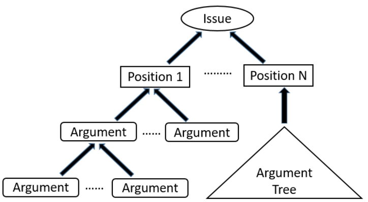
In our platform’s argumentation architecture, discussions take on a tree structure. There is a core issue at the root of each discussion, which describes the overarching discussion problem to address. Under the issue, there are several different positions for discussion in our system. Each position is a different perspective/solution which addresses or provides solutions to the parent issue. All discussions occur under a position where users can make arguments, support, or attack the parent position or other users’ arguments. In the tree structure, issues are the root nodes of the tree, the issue’s positions are first-level nodes of the tree, and all the arguments made by different users in a position are the rest nodes of the tree. Figure 1 gives a visualization of this tree structure. Participants can engage in discussion by giving arguments directly to the position itself or another user’s argument. An argument is a for/against statement, which describes the rationale relating to the position or the parent argument. Arguments can be made to support/attack the positions directly or agree/disagree with other users’ arguments in the position. When a user makes an argument, they fill out two fields. First is the text of the argument, which contains the users’ rationale for their support/attack to the parent node. Second is the level of agreement with the parent node, which indicates how much a user agrees or disagrees with the parent argument or position. Users can choose their agreement value level from a weighted scale ranging from −1.0 to +1.0 at 0.2 intervals. The sign of agreement value specifies whether the user agrees (+ ve), disagrees (- ve), or is indifferent (0) toward the parent node. And the value specifies the intensity of the agreement or how much a user agrees or disagrees with it. Here a lower value is closer to indifferent, and a higher value is closer to complete agreement or disagreement with the position. For example, an agreement value of +0.9 represents a strong level of support, and an agreement value of −0.5 represents a moderate level of disagreement with the parent argument.
Using the ICAS system, we conducted an empirical study and collected the user-opinion dataset, which we used in this work. The study was closed research and was used internally. In our study, there were four issues posing questions on ‘Guns on Campus,’ ‘Religion and Medicine,’ ‘Same Sex Couples and Adoptions,’ and ‘Government and Healthcare’ topics. Each of the issues had four different positions. These positions captured conservative, liberal, lean conservative, and lean liberal viewpoints on the topic. An expert in this field had set the Issues and positions. Users participated in the discussions of these predefined sixteen positions under four issues in our system.
2.2.Deriving viewpoint vectors using ICAS
We represent a user’s opinions in different positions using a viewpoint vector of numerical values where each element represents a user’s opinion toward the position being discussed. The user’s opinion value on a position is calculated using the agreement values from all the posted arguments by that user under that corresponding position. But not all of the arguments are made directly to the position; an argument can be made to other user’s argument in the argumentation tree. So, we first need to connect the arguments that are further down the argument tree (past the second level) to the root position since their agreement values relate to other arguments, instead of the position itself.
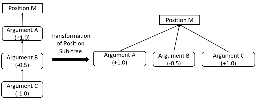
ICAS’s built-in argument reduction method [30] handles this process. The argument reduction method reduces an argument from any level of the argument tree to the first level and calculates the user’s agreement value directly towards the root position. There are four primary intuitions behind the transformation of a deep tree into a single level. Let’s assume, argument A is made to position P, and argument B supports/attacks argument A. The first case is argument A is supportive of position P. In this case, if argument B is supportive of argument A then argument B is supportive of position P. If argument B is attacking to argument A then argument B is attacking to position P. Now the second case is argument A is attacking to position P. In this case, if argument B is supportive of argument A then argument B is attacking to position P. If argument B is attacking to argument A then argument B is supportive of position P. Although these are the primary intuitions, in practice, the argument reduction technique [10] uses 25 fuzzy association rules to identify the argumentation relationship between argument B and position P through parent argument A. On a high level, these inference rules categorize the agreement values of argument B and argument A towards position p into one of the five support/attack type categories independently. These types are strong support, medium support, strong attack, medium attack, and indecisive. A fuzzy logic engine uses piecewise trapezoidal membership functions for each support/attack type and to identify the degree to which argument A and B belong to each support/attack type. These fuzzy membership values of argument A and B are used to map their weights in the fuzzy association rules. These weights and the original agreement values of argument A and B are integrated with few linear equations to determine argument B’s agreement value towards position P. Using this process, all second-level arguments are transformed into the first-level. Then, second-level arguments’ agreement towards the position p is used in a similar way to determine third-level arguments’ agreement towards the position p. In this way, the whole process is repeated iteratively level by level downward until all the arguments are transformed into the first level. Figure 2 visualizes this reduction. For a more in-depth explanation of the fuzzy logic engine and argument reduction method, refer to [3,29–31,53].
Fig. 2.
Example of an argument reduction. Argument B is reduced from the second level of the tree to the first level.
Different other algorithms compute the dialectical strength of arguments, which also transform a deep tree into a single level tree such as QuAD [4], DF-QuAD [47], Social Abstract Argumentation Frameworks [25], etc. These techniques determine the strength of an argument using a base strength of the argument and aggregated strength of the support and attack it received from other pro and con arguments. In contrast, our argument reduction technique determines agreement value to any argument/root position in the upper level.
Once all of the arguments have been reduced to the first level of the position sub-tree, then a user’s opinion toward the position can be calculated by averaging the user’s reduced agreement values to the position from all of their posted arguments. This process gives the user’s opinion value toward that position, which is added to the user’s viewpoint vector at the corresponding index. If a user does not have any arguments under a position, then their entry at that index is missing, and we want to predict this value.
2.3.Framework
Fig. 3.
Framework of the opinion prediction and group representation process.
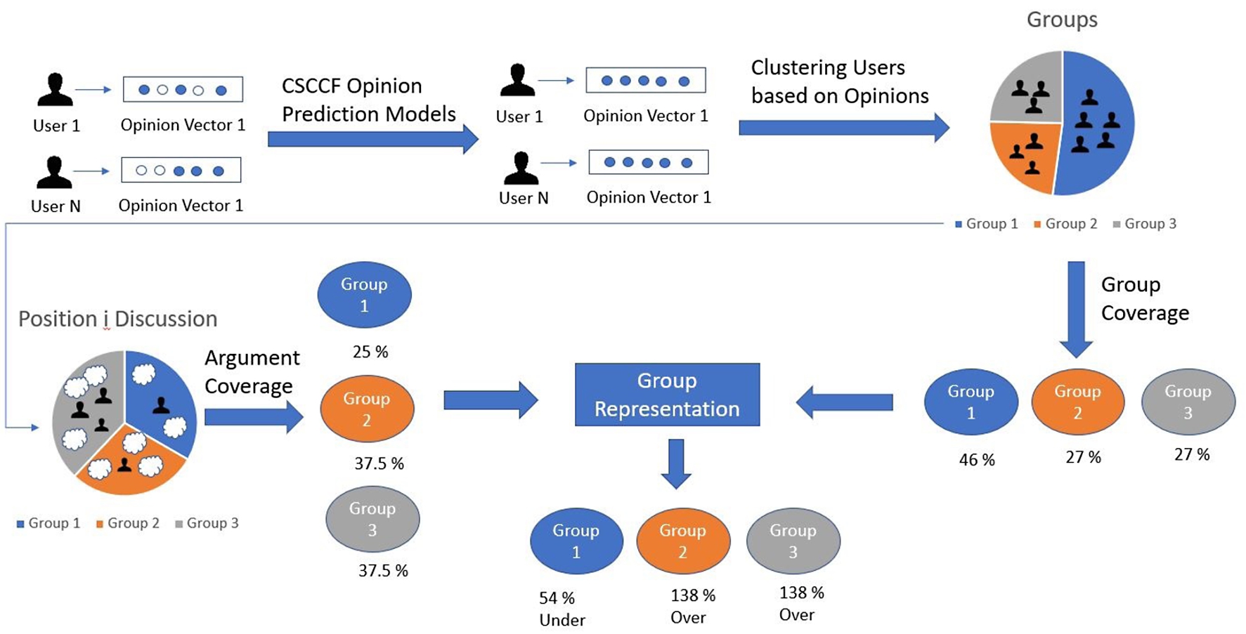
Figure 3 gives an overall idea of the whole process presented in this paper. In our system, we have opinion vectors for each user. However, some opinion values would be missing in the vector as users did not participate in all the positions. We would apply the CSCCF opinion prediction model to predict the missing opinion values. After this step, we would have a complete user-opinion vector or know users’ opinion value at each position. In the next step, we would apply the k-means clustering algorithm considering their opinions on all the positions under an issue. This process would give us different user groups with similar opinionated users in the group on an issue. Also, we measured the group coverage of these user groups based on what percentage of the total user space contains a group. In this example, group 1 contains 46%, group 2 contains 27%, and group 3 contains the system’s total users. Then we analyzed the discussions of these positions under the issue to see how much representativeness these groups have in the discussion. We measured how much of the discussion content each group contributed to the discussion. For example, we divided the user into three different groups (Group 1, Group 2, Group 3). Group 2 contributed 25%, Group 2 contributed 37.5%, and Group 3 contributed 37.5% of the total discussion content. Considering the argument coverage and group coverage, we then determined the group representation of these user groups in the position i discussion. From the results, we can see that group 2 and group 3 are overrepresented in the discussion while group 1 is underrepresented.
3.Opinion prediction model
In this section, we describe our collaborative filtering based opinion prediction model with a brief discussion on data requirement and time complexity analysis of our model. Collaborative filtering based models identify the most similar users/items and predict the rating value from similar ones’ rating patterns. In our case, items are different positions on the issues, and rating value is the user’s opinion value in the positions. We will find the most similar user to predict the opinion on the non-participated positions for a target user.
3.1.Data required for prediction
We use a viewpoint vector to represent the user opinion in different positions across issues. If a user did not participate in a position discussion, the associated opinion value would be missing in the viewpoint vector. We will use our opinion prediction model CSCCF to predict this missing user opinion. If a user (x) did not participate in a position (t), we need the following information to predict user x’s opinion value at position t: 1) Viewpoint vectors of each user in training data, 2) Viewpoint correlations of opinion values between target position t with all other positions, and 3) Viewpoint vector of the target user (User x). A viewpoint vector represents a user’s opinions in all the positions under all issues. Our model calculates viewpoint vectors for every user in training data. If there are n position in the system, the viewpoint vector of user i can be represented in the following format:
The viewpoint correlation of opinion values between a target position and all other positions is a vector of correlation values. Each value represents the correlation degree to which the opinion values in the target position relate to another position. In our system, opinions across all positions have the same value range from −1.0 to +1.0. A strong positive correlation between two positions indicates that overall users have similar opinions in these two positions, users agree or disagree with similar agreement levels. Likewise, a strong negative correlation indicates that users have opposing opinions in these two positions; if users agree in one position, they will disagree in another position with a nearly similar intensity. In contrast, a weak correlation value between two positions does not indicate any linear relationship between users’ opinions in these two positions. Correlations between position i and j are calculated using users’ opinions at position i and j with Pearson Correlation Coefficient using Eq. (1). We only included correlation values with high confidence values, correlation values with lower confidence values determined from two-tailed p-values above or equal to 0.05 are set zero.
Correlation values for a position t with other positions can be represented in the following way:
We can represent the target user (user x)’s viewpoint vector in the following vector format:
3.2.CSCCF model description
We want to predict user x’s opinion value at position t or the value of
To measure the similarity between our target user x and other users in the training dataset, we first remove any user who has a missing value at position t. The rest of the users who do not have a missing value at position t are placed into user x’s candidate set. Then we measure the similarity between user x and every user in the user x’s candidate set. We will calculate the similarity between user x and user y to demonstrate similarity calculation. The viewpoint vectors of user x and user y are
First, we remove the elements from the viewpoint vectors in which either one has a missing value. In this case,
Previously, the size of
Next, we calculate the cosine similarity between the updated viewpoint vectors
However, this similarity function does not consider the number of opinions both users have in their opinion vector. This can overestimate the similarity between users who have only a few common opinion values and may not have a similar overall opinion on issues. We adopted the following discipline technique [32] to penalize users with items less than threshold values in the similarity function and solve the overestimation problem.
Here
Our model measures the similarity between two users based on which position we are predicting. We multiply the opinion values with their correlation value with the test position. It weights or prioritizes the opinion values based on how important they are in determining the test position. If we predict another position s, the topmost similar users for target user x will be different from the similar top users when we predict position t. Our model also filters out uncorrelated opinion values by multiplying them by zero or near zero in the similarity calculation.
3.3.Time complexity of CSCCF model
In this time complexity analysis, we will measure the time complexity of our model to predict a single opinion value for one user. Suppose there are n available users, and p positions. We want to predict opinion value for a user (user x) at a position (position t). We need to compute the similarity between user x and all n available users. There are n similarity calculations in total in this process. At each calculation, we update the viewpoint vectors of size p with the correlation values. The time complexity of this approach is
4.Experiments
4.1.Empirical data description
We organized an empirical study in an entry-level sociology class in the spring of 2018 session. The class had 344 undergraduate students, and they were asked to participate in this empirical study to discuss different social issues for five weeks’ time span. The study contained four issues, and each issue had four different positions. The students were given oral and written instructions on the empirical study’s rules, how to use the system, and how to state their arguments and react or reply to other users’ arguments in the system. Also, email communications were provided to students throughout the study if they had any questions or faced any problem. The students were asked to contribute at least ten arguments in each issue. In the end, the resulting discussion had over 10000 arguments, and 309 students posted at least one argument. Ninety students participated in all the positions under four issues, which gave us the complete dataset with no missing information for different experiments. We applied for Institutional Review Board (IRB) approval from the university before conducting the study. We received the approval to conduct the study and permission to use the anonymized data for research purpose afterward. The following section describes different issues and positions for discussion in this empirical study:
4.1.1.Issue: Guns on campus
This issue posed the question: “Should students with a concealed carry permit be allowed to carry guns on campus?” and contained the following four positions for discussion:
(Position 0) No, college campuses should not allow students to carry firearms under any circumstances.
(Position 1) No, but those who receive special permission from the university should be allowed to concealed carry.
(Position 2) Yes, but students should have to undergo additional training.
(Position 3) Yes, and there should be no additional test. A concealed carry permit is enough to carry on campus.
4.1.2.Issue: Religion and medicine
This issue posed the question: “Should parents who believe in healing through prayer be allowed to forgo medical treatment for their child?” and contained the following four positions for discussion:
(Position 4) Yes, religious freedom should be respected.
(Position 5) Yes, but only in cases where the child’s life is not in immediate danger.
(Position 6) No, but may deny preventative treatments like vaccines.
(Position 7) No, the child’s medical safety should come first.
4.1.3.Issue: Same sex couples and adoption
This issue posed the question: “Should same sex married couples be allowed to adopt children?” and contained the following four positions for discussion:
(Position 8) No, same sex couples should not be allowed to legally adopt children.
(Position 9) No, but adoption should be allowed for blood relatives of the couple, such as nieces/nephews.
(Position 10) Yes, but same sex couples should have special vetting to ensure that they can provide as much as a heterosexual couple.
(Position 11) Yes, same sex couples should be treated the same as heterosexual couples and be allowed to adopt via the standard process.
4.1.4.Issue: Government and healthcare
This issue posed the question: “Should individuals be required by the government to have health insurance?” and contained the following four positions for discussion:
(Position 12) No, the government should not require health insurance.
(Position 13) No, but the government should provide help paying for health insurance.
(Position 14) Yes, the government should require health insurance and help pay for it, but uninsured individuals will have to pay a fine.
(Position 15) Yes, the government should require health insurance and guarantee health coverage for everyone.
The four positions under each issue are categorized in advance as conservative, moderately conservative, moderately liberal, and liberal viewpoints on the issue.
4.2.Methods to test against
We implemented different popular opinion predictive techniques and compared their accuracy with our CSCCF model using the collected empirical dataset. These methods include one neural net, two matrix-factorization based approaches, and six different memory-based collaborative filtering models. The only difference between these CF models and our CSCCF model is the similarity calculation between two users. CSCCF and these CF models predict Opinion value from the most similar users in the same way. The following section briefly describes all the comparison models.
4.2.1.Cosine Similarity based CF (CSCF)
This method used the Cosine similarity between the original viewpoint vectors to select the topmost similar users. For two users x and y, their similarity is measured using their agreement vectors
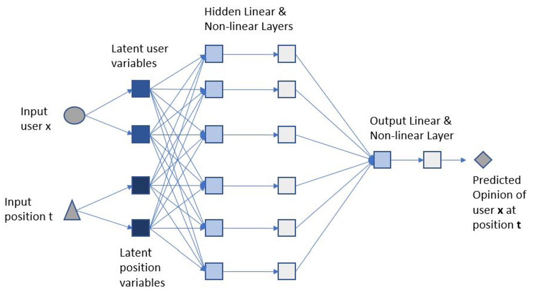
Fig. 4.
Neural network architecture.
4.2.2.Neural network
Neural networks have been used extensively in research to solve complex problems, and have been modified to solve collaborative filtering problems. The neural network we implemented is a model-based hybrid collaborative filtering model through a neural network approach, as described in [56]. This model captures the essence of both content-based filtering and collaborative filtering models: content information, preference, similarity, or correlation between the users or items from the dataset. This model uses a set of latent factors/embeddings for both users and items through a neural network approach. It employs two different kinds of latent input variables. First, the latent variables for known features of user/item, which take advantage of content-based filtering. Second, the latent input variables to capture the correlation/preference/similarities for both user/item in the dataset. These latent input variables represent a user and item, which are input to our neural network model. The output of this model the associated rating for the input user and item. During the training phase, the neural net model learns the weights and latent input variables simultaneously. These latent variables are updated with respect to error using a generative backpropagation algorithm the same way internal weights are updated. The neural network model can be trained in the three phases. In the first phase, the models compute an initial estimation of the latent input variables without updating the model’s internal weights. And based on the error on the output, it updates the latent input variables. The updated latent input variables are kept fixed in the second phase. This phase updates the weights and tries to converge with fixed latent input variables so that model can train without the moving input. In the third phase, the model updates the weights and input together. All these three phases use stochastic gradient descent. The first two phases provide a good initial estimation of the input and model weights, which helps the gradient descent figure out a better local optimum. For more details on this technique, please refer to [56].
We experimented with different numbers of latent inputs for both users and positions in our neural network implementation. We iterated through 1 latent input to 16 latent inputs for each user and each position and evaluated the neural network model’s performance. We got the best result when we used two latent variables for each user and two latent variables for each position. So, in total, these four variables (two for one user, two for one position) were the input in our neural network. And the output is the predicted opinion of the input user on the input position (one output). Figure 4 shows the architecture of our neural network model. We used this topology in our neural net implementation: linear layer (4, 6) ⩾ Tanh layer (6, 6) ⩾ linear layer (6, 1) ⩾ Tanh layer (1, 1). The first numbers represent the input dimension, and the second number represents the output dimension in each layer. The first layer is a linear layer with input dimension 4 representing the latent input variables. Tanh is the activation function applied to the dense hidden layer. Then a final linear layer is applied with the input of 6 dimensions and output of 1 dimension. This output is the predicted opinion value of the input user and position. The model attempted to predict the user’s opinion, given a user’s latent vector and a position’s latent vector. In the training time, the neural net used stochastic gradient descent to update the inputs and weight parameters, and sum squared error (SSE) was used to optimize the neural net.
We experimented with both latent and known features for the user and position in our implementation. The best result we got, using only the latent features for both user and position. On the latent variables, we tried various input layer vector sizes, the best result we got when the latent vectors were at length 2 for both users and positions. These four variables (two for one user, two for one position) were the input in our neural network, and the output is predicted opinion (one output for a position). Also, we trained our neural net model with one phase training for simplicity instead of training the weights and latent input variables in three phases.
4.2.3.Matrix factorization
Matrix factorization is a popular predictive method that decomposes a matrix into multiple matrixes such that when they are multiplied together, it returns the original matrix. We implemented a matrix factorization based collaborative-filtering model. In our case, the original matrix is the user (U) – position (D) matrix (
Here,
4.2.4.Probabilistic matrix factorization
This is a probabilistic matrix factorization based collaborative-filtering model. We implemented Probabilistic Matrix Factorization (PMF) as described in [37]. PMF is a Matrix Factorization based model that uses a probabilistic linear model and considers Gaussian observation noise. Like with the neural network and matrix factorization, PMF assumes users and positions have latent vectors of size k. However, unlike matrix factorization, the latent matrices are drawn from a normal distribution, determined by each row’s means and variances in the original matrix. So, when they are multiplied together, the resulting matrix is also normally distributed. The resulting matrix is derived in (8).
Here, α is the learning rate for the update of model parameters. β, and γ is the regularization terms for user and item factors. The values of α, β, and γ were 0.02, 0.025, and 0.002 respectively in our experiment. We used a Java Platform Standard Edition 8’s built-in normally distributed random number generator [48] with a mean of 0.0 and standard deviation of 1.0 for value initialization in our PMF implementation.
4.2.5.Spearman Rank Correlation Similarity based Collaborative Filtering (SRCSCF)
This CF model uses the items’ rank/index instead of items’ values in the similarity calculation. We used the original viewpoint vector (
4.2.6.Jaccard Similarity based Collaborative Filtering (JSCF)
This model measures the similarity between two users based on the number of items they rated with similar values. In our case, we rounded the opinion agreement values from the original viewpoint vector
4.2.7.Normalized Mean Squared Difference Similarity based Collaborative Filtering (NMSDSCF)
This model measures the Mean squared difference between the two original viewpoint vector
4.2.8.Jaccard and Mean Squared Difference Similarity based Collaborative Filtering (JNMSDSCF)
This method integrates the jaccard similarity and mean squared difference similarity to measure the similarity between user x and user y using the following equation:
4.2.9.Pearson Correlation Similarity based Collaborative Filtering (PCSCF)
This model calculates the Pearson correlation coefficient value from original viewpoint vectors (
4.2.10.Constrained Pearson Correlation Similarity based Collaborative Filtering (CPCSCF)
This model is a modification of Pearson Correlation based Collaborative Filtering. It uses the midpoint instead of the mean rating value to measure the correlation and use it as the similarity between user x and user y.
4.3.Experimental results
4.3.1.Predicting opinion in a single position with different level of sparsity
In this experiment, we analyzed the accuracy of our CSCCF and other baseline models in terms of Mean Absolute Error (MAE) when they predict user opinion in a single position. MAE value is calculated from the actual and predicted user opinion value at a particular position. We conducted this experiment in two variations of the dataset to evaluate accuracy in different level of sparsity. One variation of the dataset is the complete user-opinion dataset, where all users have opinion values in all the positions, and there are no missing opinion values. We refer to this dataset as ‘complete dataset (without any missing opinion values).’ Another variation is the entire user-opinion dataset, which is the original dataset collected from the empirical study. As many users did not participate/express opinions in many discussions, so this dataset contains missing opinion values. We refer to this dataset as ‘entire dataset (with missing opinion values).’ We performed cross-validation on both datasets and averaged the MAE value over two repetitions. In each repetition, we performed five iterations of evaluations of the models. We randomly divided the dataset into two parts in each iteration, 80 percent as the training data and 20 percent as the testing data. Also, we made sure we do not repeat the same data into the test set in between the iterations and repetitions. Using this test environment, we evaluated the accuracy for each position and averaged the MAE values. This MAE value across all positions is reported in the experimental results. The following two sections contain the result of this experiment.
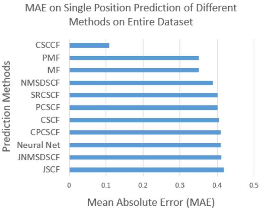
Accuracy on entire dataset (with missing opinion values). Figure 5 contains the accuracy values of different models in terms of MAE. From the results, we can see that CSCCF outperformed every other model in every position. The average MAE value of the CSCCF model is 0.109, whereas the MAE value from the second best-performing model PMF is 0.350. The MAE value from all other models lies in between 0.351 to 0.42. The MAE value for all other models was in between a narrow range. In contrast, the CSCCF model shows visible improvement filtering out uncorrelated opinion values and weighting related opinion values as per their importance to predict the test position. For example, when we measured the MAE value for position 14, all comparison models hovered between 0.31 and 0.39, but the CSCCF model achieved the MAE value of 0.09. From this experimental result, we can see that the CSCCF model outperformed all baseline comparison models, which show the importance of weighting the opinion values by their correlation values with the test position in the similarity calculation.
Fig. 5.
MAE on predicting single position of different models with on entire dataset.
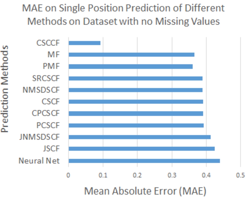
Accuracy on the complete dataset (without any missing opinion values). In this experiment, we compared the accuracy of CSCCF and other baseline models on the complete user-opinion dataset, where every user had opinion value in every position. Figure 6 contains a summary of this experiment. Compared to the MAE value on the entire dataset, the MAE value of the CSCCF model decreased to 0.093 on this complete dataset. However, the MAE value of the second-best performing model, which is PMF in this experiment got increased to 0.365. With few exceptions, the MAE of the comparison models tended to decrease in this complete dataset, especially for the CF-based models. So, less sparse data in the user feature vector is helping to find similar users more effectively. The MAE value of Matrix Factorization, Probabilistic Matrix Factorization, and Neural Net models increased in this dataset compared to the entire dataset. We think these models are suffering to figure out the latent relationship between users to their opinions because of the smaller data size in this dataset. Which is why the MAE value got increased compared to their MAE values on the entire dataset. The experimental result shows that the CSCCF model outperformed other models not only in the sparse dataset, it also outperformed these models in a complete dataset with no missing values.
Fig. 6.
MAE on predicting single position of different models with no missing values.
Experimental result analysis. The improvement over CF-based models, especially the Cosine Similarity based CF (CSCF), shows the usability of position correlations in similarity calculation. In CSCF, each position agreement value in the viewpoint vector has a similar priority when we measured the similarity between two users. Whereas in our CSCCF model, each opinion value is weighted according to the correlation with the target position. Our model CSCCF also outperformed Neural Net, Matrix Factorization, and Probabilistic Matrix Factorization models. We think limited data size and missing values within this limited dataset are the main reason for the underperformance of the neural network models. As most of the users did not participate in all the position discussions, our dataset contained many missing values. At most, each user can have a maximum of 16 opinion values. So, there are not a lot of values to learn about users and discover their patterns. As a result, the latent features and relationships learned by the neural network and matrix factorization-based models are most likely to be underdeveloped. It may have contained little meaningful information to learn about user-opinion space and exploit those learned relationships for effective opinion prediction resulting in lower accuracy.
Our model handles the data sparsity issue by utilizing the global correlation values calculated from training data and using them for each user with their limited available information. As there was not much data to learn about the individual user, our model made the best use of data by integrating the global correlation with users’ personalized data points.
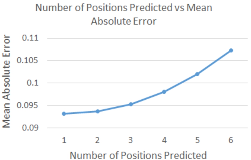
4.3.2.Predicting opinion on multiple positions across issues
In this experiment, we evaluated the CSCCF model’s accuracy when it predicts user opinion values at two to six positions simultaneously. With a fivefold, two repetitions and 80:20 ratio for training and test data, we used all possible combinations while testing at each number of positions. For example, when we predict two positions simultaneously, we experimented with all possible 120 combinations of two-position indices;
Fig. 7.
MAE on different number of positions prediction.
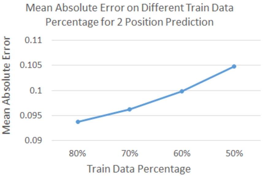
4.3.3.Predicting opinion with different training data size
In our model, we calculate the correlation value between positions from the training data; the number of samples in the training data should impact the overall accuracy of the CSCCF model. We evaluated the impact of varying training data sizes on the overall accuracy of the CSCCF model in this experiment. We divided the training and testing data into different ratios such as (80:20), (70:30), etc. and measured the MAE values at different training and testing data ratios. Figure 8 shows our model’s MAE value on the dataset with no missing values at different training data percentages. The smaller the training size, the larger the MAE value gets as some of the most similar users might be missing from training data. This rate increases after we include 70% of the users as training data but remains within 0.1 until we included 50% of the users in the training set. This test shows that even smaller sizes of training data do not affect the model drastically as a whole; it might affect individual positions.
Fig. 8.
MAE on different train data percentage.
4.3.4.Predicting opinion by the baseline comparison models on the filtered dataset by different correlation degree with different level of sparsity
Our CSCCF model weighs the opinion values according to their correlation values with the test position in the similarity measurement between users. This step filters out uncorrelated opinion values and is the major contributing factor for the high accuracy achieved by the CSCCF model. In this experiment, we evaluated the impact of filtering the dataset by different correlation degrees on the baseline models’ overall accuracy and whether filtering enables these baseline models to outperform the CSCCF model.
To test this approach, we calculated the correlation values between the positions from the training data. Then we used the correlation values to filter out positions in the similarity calculation of collaborative filtering models. On a particular threshold correlation value, positions with greater or equal threshold correlation values were only used when calculating the similarity between users. In MF and PMF, agreement values in positions with lower correlation values with the test position were removed from the user-item matrix. This step will ensure that these values will not be used by these methods to predict the test position. The neural net model we implemented uses latent feature variables to learn about individual users and positions. In training time, for each (user, agreement value at a position) pair, it updates the associated latent user vector and latent position vector. At the end of the training, we have the final latent user vectors for each user and latent position vectors for each position. In testing time, for a (user, position) value pair, the associated latent vectors of user and position are loaded to predict the opinion. The idea of incorporating correlated data points in training time is not valid here, as for a (user, position) pair
Fig. 9.
MAE on entire dataset with different threshold correlation values.
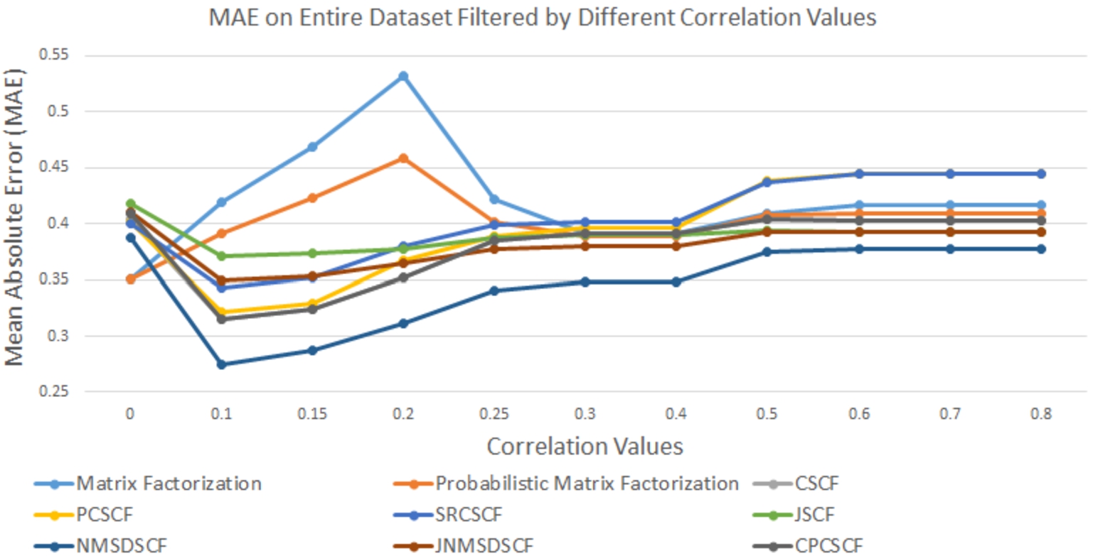
Accuracy on the entire dataset (with missing opinion values). We filtered the entire user-opinion dataset by different correlation values and measured the MAE values in this experiment. Figure 9 contains a summary of this experiment. For all CF models, the lowest MAE value was achieved by filtering the dataset with a threshold correlation value of 0.1; the MAE value at this point is significantly smaller than when the unfiltered dataset was passed to the CF-based models. After the 0.1 threshold correlation point, increasing correlation values resulted in higher MAE values. The original dataset contains lots of noisy and irrelevant values. By filtering the dataset at the correlation value of 0.1, noisy values got removed from the dataset, which triggered the lowest MAE value for the collaborative filtering models. But further removing more data points by threshold correlation values makes the data size too small for collaborative filtering models to find users with reasonable similarity to derive or predict agreement value with high accuracy. The lowest MAE value was achieved by feeding the entire unfiltered dataset to both MF and PMF models. With each filter applied by threshold correlation value, the dataset got too small and probably lost meaningful information to determine the latent features and relationships between users and items. This is why the MAE value was best when data was unfiltered than the filtered ones at different correlation values. None of these baseline models achieved high accuracy as the CSCCF model at all the threshold correlation degree. This experiment shows that even filtering the dataset did not enable these baseline models to outperform CSCCF’s accuracy on the entire dataset.
Fig. 10.
MAE on complete dataset with different threshold correlation values.
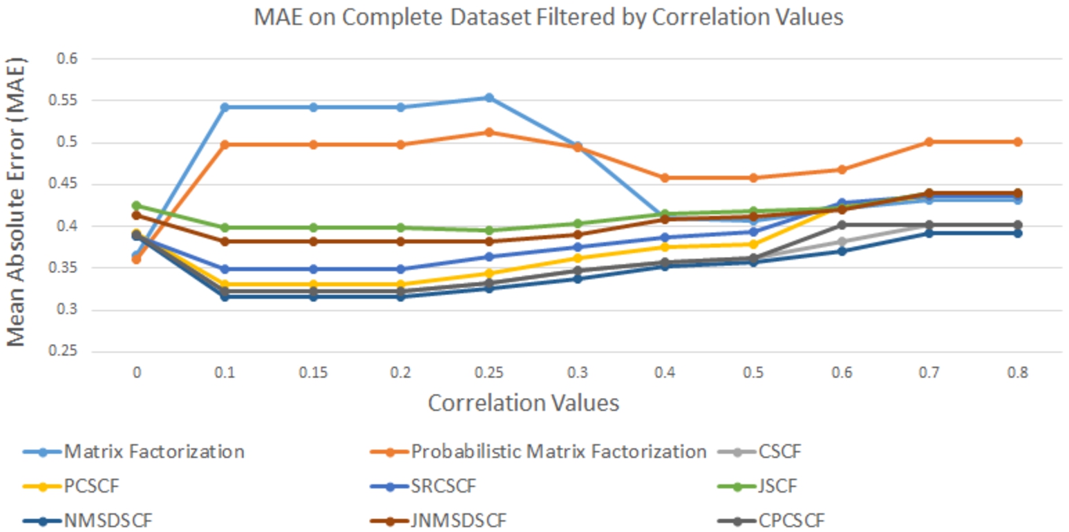
Accuracy on the complete dataset (without any missing opinion values). In this experiment, we filtered the complete dataset with no missing value and fed them into different baseline models. Figure 10 contains a summary of this experiment. Matrix factorization and Probabilistic Matrix Factorization followed a similar pattern of the MAE values at different threshold correlation values. For both MF and PMF, the best MAE value was achieved by feeding the unfiltered dataset to the models. This complete dataset is already small in size; further filtering is making this dataset smaller in size. The smaller data size affects the learning process in MF and PMF, resulting in lower accuracy in the filtered dataset than the unfiltered one. For all CF models except JSCF, the best MAE value was achieved at the threshold correlation value of 0.1; after that, the MAE value increased gradually with increasing correlation values. None of the models outperformed CSCCF’s accuracy on the complete dataset in this experiment.
4.3.5.Predicting opinion by the baseline models on the preprocessed dataset with different level of sparsity
In our CSCCF model, we multiplied the opinion values by their correlation values with the test position in the similarity measurement to prioritize data points according to their relevance with the test position. In this experiment, we analyzed the impact of feeding the weighed datapoints by correlation values to different baseline models and whether this step enables any of these models to outperform the CSCCF model. To analyze this scenario, we calculated the correlation values between different positions from the training data. For a particular test position, we multiplied the correlation values with the original agreement values in the training data. Then we measured the average MAE value on the modified dataset using the 80:20 training testing data ratio and fivefold, two repetition cross-validation setup.
Figures 11 and 12 contain the summary of this experimental result on the entire dataset (with missing opinion values) and the complete dataset (without any missing opinion values). On the entire dataset, MF and PMF achieved the lowest MAE value compared to other collaborative filtering models. However, on the complete dataset, MF and PMF achieved the worst MAE value out of all prediction models, and NMSDCF achieved the lowest MAE value. The correlation-based CF models use correlation values as the similarity between users or items. The relationship cannot be extracted by further calculating correlation values on the modified by correlation data. This is the reason for the worse performance of these correlation-based CF models. Even though the values were multiplied by the correlation values on the complete dataset, the smaller size of the dataset is the reason we think MF and PMF did not achieve as low MAE value as on the entire dataset. This also strengthens the fact that MF and PMF models need more data to extract latent relationships between users to items to predict with high accuracy. None of these models outperformed CSCCF even with the modified dataset, which signifies the importance of weighing the data in similarity calculation as performed by the CSCCF model.
Fig. 11.
Mean absolute error of different models on modified entire dataset.
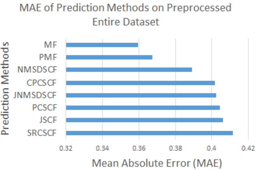
Fig. 12.
Mean absolute error of different models on modified complete dataset.
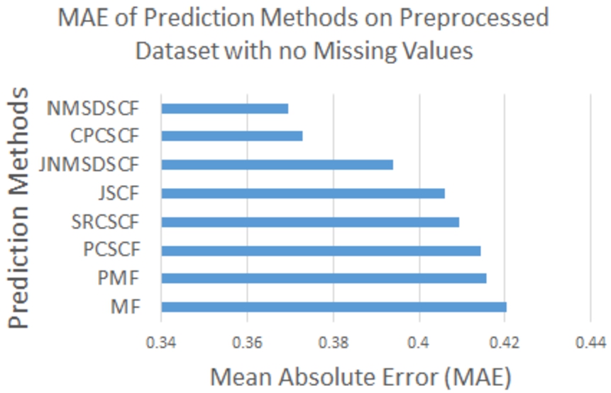
Fig. 13.
MAE by CSCCF model on two datasets at different threshold correlation values.
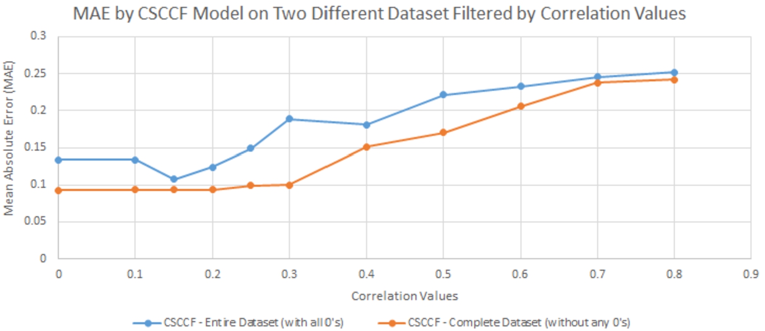
4.3.6.Determining threshold correlation values for reasonable accuracy by CSCCF model
Our CSCCF model relies on the correlation values on the dataset to predict opinion with reasonable accuracy. In this experiment, we tried to determine the threshold correlation value that needs to be present in the dataset to achieve high accuracy by the CSCCF model. At first, we measured the MAE value by the CSCCF model both on the entire dataset (with missing opinion values) and on the complete dataset (without any missing opinion values). Then, we filtered both datasets by different correlation values and measured the corresponding MAE values to determine the threshold correlation value. Figure 13 summarizes the result of this experiment. From the results, we can see that the CSCCF model achieved the highest accuracy when both datasets were filtered by a correlation degree of 0.15. Although filtering by the higher correlation value should yield to lower MAE value, it also reduces the percentage of data used in the prediction model. This is the reason filtering by higher correlation is resulting in higher MAE values. A balance between filtering by a correlation degree and the percentage of data used by the model needs to be considered. In our case, we utilized 80 percent or above of available data when we achieved the lowest MAE values, and threshold correlation values were between 0.1 to 0.2. These threshold correlation values might not remain valid in another dataset. This experiment needs to be performed to determine the optimal threshold value for the filtering process before utilizing the threshold correlation value in the CSCCF model. If we can determine the threshold correlation value
5.Opinion prediction model application
CSCCF opinion prediction model can be used to analyze different social phenomena in our ICAS system. In this section, we analyzed Group Representation phenomena to showcase how the opinion prediction model can be used in our system.
5.1.Group representation phenomena analysis
In our system, users contribute to the discussion by posting numerous arguments. The arguments generally contain the opinions, rationale, ideas, etc. favoring the participating user’s opinion or perspective on the issue. On a collective level, the entire discussion content represents the viewpoint, opinions, rationale, etc. of the participating users. However, typically users with different perspectives do not participate in the discussion proportionally. If a particular opinionated group participates in the discussion mostly, they will contribute to most of the discussion content. The overall tone of the arguments in the discussion might favor their opinion values. And if a particular opinionated user group does not participate in the discussion, the discussion would not represent their viewpoint at all. When a new user reads the discussion, he/she might get the idea that the majority of the people have this one particular kind of opinion on this issue as the majority of the arguments favors this viewpoint. However, this may not be the real scenario. Users with different perspectives other than the participated ones did not have significant enough participation in the discussion to be noticed or give people ideas about their opinions, ideas, viewpoint, etc. on the issue. This may create some bias to the reader’s mind as the discussion content is not proportionally representative of different opinionated user groups.
We can measure how much a particular opinionated group is represented in the discussion to inform the readers how representative a discussion is of a user group. If a user group contributes a proportionate number of arguments in the discussion, then that discussion is ideally representative for that user group. Proportionate means that a user group’s number of arguments matches their share of total users in the platform. For example, suppose a user group contains 20 percent of the total users and contributes 20 percent of the discussion’s arguments. In that case, that discussion is ideally representative of that user group. If a user group contributes more arguments than their proportionate share, then the discussion is over-representative of that user group. If a user group contributes fewer arguments than their proportionate share, then that discussion is under-representative of that user group. We will measure this phenomenon using the “Group Representation” metric.
To measure this group representation metric, we need to group users based on their opinion on an issue. Then for each group, we need to measure the percentage of the total users this group covers. We will also measure the portion of the discussion content each group contributed to the discussion. Using the user and argument coverage, we will measure the group representation value for each opinionated group in the discussion. We defined the following term “User Coverage” to measure the portion of the whole user-space a particular group covers.
We defined another term, “Argument Coverage,” to measure the portion of arguments in the discussion a particular group contributed to convey their idea, beliefs in the discussion. We assumed that all arguments have similar strengths in the ‘Argument Coverage’ metric. Various factors can contribute to the status/value/strength of an argument. For example, the length of an argument, the number of replies/reactions to the argument, depth of the argument in the argumentation tree, topics/rationale present the argument, level of replies to the argument, etc. and different hidden factors that capture users attention. It is challenging to identify all these factors and analyze which factor is more important than others for the ‘Argument Coverage’ metric. We would need another model to identify these factors and measure these factors’ exact importance/weight. So, we assumed that all arguments are equivalent in terms of their importance in the ‘argument coverage’ metric for simplified calculation with the following equation:
5.2.Clustering users with traditional imputation approach
We imputed users’ missing opinion values at different positions using the mean agreement value from all users in that position. Then, we applied the K-Means clustering algorithm to group users based on their opinion on an issue with a different number of clusters and evaluated the clustering quality with the Silhouette score. For the ‘Guns on Campus’ issue, the best clusters were found when the users were divided into five groups. For ‘Religion and Medicine,’ ‘Same Sex Couples and Adoption,’ and ‘Government and Healthcare’ issues, the best clusters were found when the users were divided into six, four, and five groups, respectively.
Table 1
Group characteristics for gun issue using column mean as missing value
| Group no | Group size | G1: Value | G2: Value | G3: Value | G4: Value |
| 0 | 39 | −0.42 | 0.11 | 0.37 | 0.52 |
| 1 | 119 | 0.27 | 0.11 | 0.12 | −0.43 |
| 2 | 51 | 0.70 | −0.55 | −0.4 | −0.75 |
| 3 | 39 | 0.86 | 0.24 | −0.6 | −0.8 |
| 4 | 60 | −0.50 | 0.36 | 0.56 | −0.43 |
Table 1 contains the clustering result in the Guns on Campus issue. In this issue, we have position 0 (G1), position 1 (G2), position 2 (G3), and position 3 (G4), and the best clusters we got when the number of clusters was defined at 5. The mean agreement value for G1, G2, G3, and G4 positions are 0.20, 0.11, 0.12, −0.43, respectively. In general, groups merged users with missing values and users with near missing values and put them in one group. Group 0 is made of users with missing values and users with near missing values at the G2 position. Users of Group 4 have either missing values or near missing values at the G4 position. Group 1 is the largest group out of 5 groups; its users have missing values at G2, G3, and G4 positions or their agreement values are near the missing values. We also observed the same phenomena of grouping users with near and missing opinion values together on other issues. We also tried imputing the missing values with median agreement value and the most frequent agreement value in a position. The resulting pattern is the same as imputing the missing values with mean agreement value. Clustering algorithms treat the users with missing values and users with near missing values in a similar way and put these users into one group. If these users did not have missing values, they might not be in the same group. So, the clustering algorithms’ output groups are not reliable and contain incorrect groupings of many users.
5.2.1.Clustering with predicted values from CSCCF
We imputed the missing values using the CSCCF for each missing opinion values in the dataset. On the complete dataset (without any missing opinion values), we then applied the K-Means clustering algorithms to group users based on their opinion within an issue. This clustering results we got this time are much improved and better than the three missing value imputation methods discussed in the earlier section. This time the clustering algorithm did not put the users with missing values at a position together into one group. Also, the output groups have definite characteristics than the previously generated opinionated user groups. The following Table 2 contains the group results generated from the clustering algorithm with each group number, their size, overall group opinion (average agreement value) at four positions (Positions 0 (G1), Position 1 (G2), Position 2 (G3), and Position 4(G4)). In the last row, it also shows the overall user opinion (average agreement values at four positions) of all users in the system.
Both Group 0 and Group 3 strongly support that college campuses should not allow students to carry firearms under any circumstances. But Group 0 does not hold this belief for exceptional cases of allowing to carry concealed firearms by those who receive special permission. In contrast, Group 3 does not favor for these exceptional cases. However, Group 0 and Group 3 disagree that a concealed carry permit or additional training would validate students to carry guns on campus. Group 2 is more approving for students carrying guns but with restrictions like special permission, additional training, or test than banning guns on campus totally or giving students full freedom to carry guns on campus. Group 1 has a similar opinion to group 2, but they support giving students’ freedom to carry guns on campus. Group 4 is the largest of these five groups in user numbers; supports mostly that carry permit is not enough; some restrictions should be applied to allow students to carry firearms on campus.
Table 2
Statistics of different user groups for gun issue
| Group no | Group size | G1: Value | G2: Value | G3: Value | G4: Value |
| 0 | 61 | 0.75 | 0.35 | −0.2 | −0.75 |
| 1 | 43 | −0.53 | 0.29 | 0.37 | 0.40 |
| 2 | 71 | −0.30 | 0.34 | 0.54 | −0.44 |
| 3 | 47 | 0.75 | −0.55 | −0.6 | −0.8 |
| 4 | 86 | 0.47 | 0.05 | 0.36 | −0.55 |
| Overall | 308 | 0.37 | 0.18 | 0.23 | −0.55 |
From the above discussion, we have shown how the prediction model helped us identify user groups with definitive characteristics compared to the previous missing value imputation results. With these defined user groups, we analyzed user group representation in the various issue discussions.
5.3.Group representation experimental results
This section contains the group representation experimental results in the four issues in our system. We described the group representation experimental results in detail in one position and provided an overall summary of the four positions in each of the issues.
5.3.1.Result on guns on campus issue
Table 3 contains the group representation results for five different groups in position 2 discussion. From the results, we can see that Group 0 and Group 4 are under-represented, whereas Group 1, Group 2, and Group 3 are over-represented in the discussion of position 2. Although Group 4 is the largest group in user size but did not have the highest number of arguments in the discussion. Even though Group 2 was not the largest group user size-wise, they are the largest group represented in the discussion according to the number of arguments. So, they are over-represented in the discussion.
Table 3
Group representation of different user groups for guns on campus issue at position 2
| Group no | Group size | Group percentage | Number of arguments | Argument percentage | Group representation | Representation |
| 0 | 61 | 0.198 | 97 | 0.167 | 0.844 | Under-represented |
| 1 | 43 | 0.140 | 85 | 0.146 | 1.050 | Over-represented |
| 2 | 71 | 0.230 | 153 | 0.263 | 1.144 | Over-represented |
| 3 | 47 | 0.152 | 106 | 0.183 | 1.198 | Over-represented |
| 4 | 86 | 0.279 | 139 | 0.240 | 0.858 | Under-represented |
Fig. 14.
Group representation of different groups at different positions of gun issue.
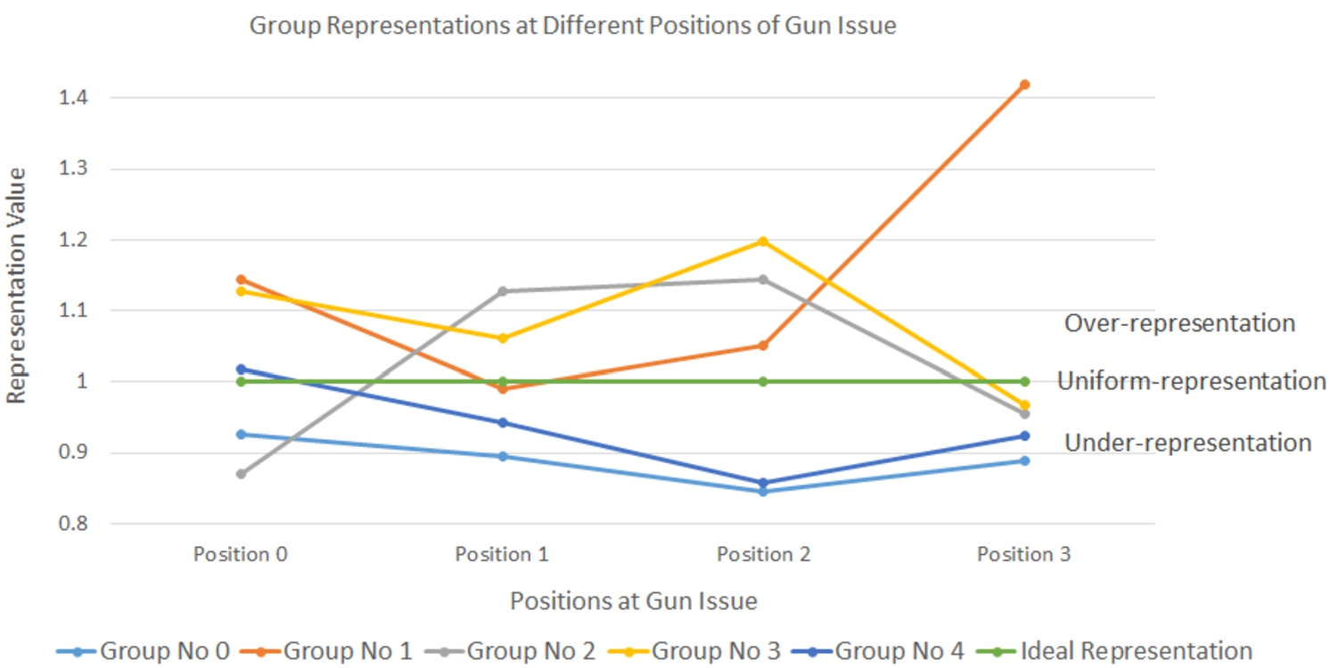
Table 3 presents group representation results of user groups only in one position (position 2). Figure 12 presents the group representation experimental results of user groups at all four positions (positions 0, 1, 2, and 3). From Fig. 14, we can see whether a group is over or under-represented in the discussion at all four positions on the gun issue. Group 0 is under-represented in all four positions, whereas Group 1 is over-represented in all positions except position 1. Group 2 is under-presented in position 0 and position 3, but over-represented in position 1 and position 2. Group no 3 is over-represented in all positions except position 3, whereas Group 4 is under-represented in all positions except position 1. In summary, Group 1 is the most over-represented, and Group 0 is the most under-represented group in all the discussions.
5.3.2.Result on religion and medicine issue
There are six user groups (Group 0, Group 1, Group 2, Group 3, Group 4, and Group 5) in this issue. Table 4 contains the opinions of these user groups in the discussion of position 4 (R1), position 5 (R2), position 6 (R3), and position 7 (R4). Group 3 holds conservative viewpoints on this issue. They agree that a child’s medical safety should not come first over the religious freedom of denying any medical facilities. They agree that religious freedom should always be respected, only not when the child’s life is in immediate danger. Group 0 is overall in the middle. They agree that religious freedom should be respected, and parents may deny preventative treatments like vaccines. However, their opinion prioritizes support for child’s medical safety, rather than religious freedom. Group 1, Group 2, Group 4, and Group 5 hold liberal viewpoints on this issue. These groups agree with the child’s medical safety should come first and disagrees with the idea that religious freedom should be respected. They disagree that parents may deny preventative treatments like vaccines. Group 4 has the strongest association; Group 5 has the second-highest strong association, and Group 1 the least strong association in their opinions among these four groups.
Table 5 contains the group representation results in the discussion of position 6. From the results, we can see that Group 0, Group 1, and Group 2 are under-represented in the discussion of position 2. Whereas Group 3, Group 4, and Group 5 are over-represented in the discussion of position 2. Group 3 is the most over-represented group in this discussion. This group contains only 12% of the total users but contributes around 15% of the discussion’s total arguments. Group 1 is the least under-represented group in the discussion. This group contributes only 14% of the discussion content while they comprise 16.6% of total user space.
Table 4
Statistics of different user groups for religion and medicine issue
| Group no | Group size | R1: Value | R2: Value | R3: Value | R4: Value |
| 0 | 52 | 0.29 | 0.6 | 0.4 | 0.57 |
| 1 | 51 | 0.28 | 0.12 | −0.29 | 0.59 |
| 2 | 78 | −0.4 | 0.47 | 0.26 | 0.63 |
| 3 | 37 | 0.28 | 0.23 | 0.05 | −0.25 |
| 4 | 41 | −0.53 | −0.2 | 0.04 | 0.89 |
| 5 | 49 | −0.43 | 0.4 | −0.7 | 0.86 |
Table 5
Group representation of different user groups for religion and medicine issue at position 6
| Group no | Group size | Group percentage | Number of arguments | Argument percentage | Group representation | Representation |
| 0 | 52 | 0.17 | 86 | 0.16 | 0.95 | Under-represented |
| 1 | 51 | 0.16 | 75 | 0.14 | 0.84 | Under-represented |
| 2 | 78 | 0.25 | 130 | 0.24 | 0.97 | Under-represented |
| 3 | 37 | 0.12 | 82 | 0.15 | 1.24 | Over-represented |
| 4 | 41 | 0.13 | 71 | 0.13 | 1.01 | Over-represented |
| 5 | 49 | 0.16 | 89 | 0.17 | 1.05 | Over-represented |
Table 6 contains summarized Group Representation (GR) values of in the discussion of position 4 (R1), position 5 (R2), position 6 (R3), and position 7 (R4). From the results, we can see that group 4 is the most over-represented in the discussions of Religion and Medicine issue. This group is over-represented in all the discussions at four positions under this issue. Whereas, group 1 is always under-represented in any discussion of this issue. The other groups are over-represented in some positions, while under-represented in other positions.
Table 6
Group representation values of users groups at different position discussions of religion and medicine issue
| Group no | R1: GR value | R2: GR value | R3: GR value | R4: GR value |
| 0 | 1.01 | 1.07 | 0.96 | 1.13 |
| 1 | 0.76 | 0.70 | 0.85 | 0.85 |
| 2 | 1.09 | 1.10 | 0.98 | 1.01 |
| 3 | 1.13 | 1.19 | 1.25 | 1.05 |
| 4 | 0.98 | 1.00 | 1.00 | 0.85 |
| 5 | 0.99 | 0.93 | 1.05 | 1.09 |
5.3.3.Result on same sex couples and adoption issue
There are four user groups (Group 0, Group 1, Group 2, and Group 3) in this issue. Table 7 contains the opinions of these user groups in the discussion of position 8 (S1), position 9 (S2), position 10 (S3), and position 11 (S4). Only Group 0 holds conservative opinions on the Same Sex Couples and Adoption issue. This group agrees that same-sex couples should not be allowed to adopt children legally and not be treated as heterosexual couples. Whereas Group 1, Group 2, and Group 3 hold liberal opinions on this issue. They support equal treatment of same-sex and heterosexual couples regarding adopting children. Also, they oppose any legal forbidding for same-sex couples to adopt children. However, they differ how strong their opinions are. Group 1 has the strongest, Group 2 has in the middle, and Group 3 has the least strong opinions in the liberal viewpoint on this issue.
Table 8 contains the group representation results of user groups in the discussion of position 10. In this issue, we have four user groups. Group 0 and Group 1 are the over-represented groups; Group 1 and Group 2 are the under-represented user groups. Group 3 is the most over-represented user groups; it contributes more share of discussion content (27%) than its share of total user-space (21.4%). Group 2 is the most under-represented user group in the discussion. This group contains the largest share (35%) of total users but does not contribute proportionally to the discussion content. It only provides 31.5% of the total discussion content.
Table 7
Statistics of different user groups for same sex couples and adoption issue
| Group no | Group size | S1: Value | S2: Value | S3: Value | S4: Value |
| 0 | 37 | 0.62 | 0.3 | −0.10 | −0.6 |
| 1 | 95 | −0.73 | −0.6 | −0.69 | 0.9 |
| 2 | 110 | −0.79 | −0.55 | 0.2 | 0.8 |
| 3 | 66 | −0.20 | 0.08 | 0.15 | 0.48 |
Table 8
Group representation of different user groups for same sex couples and adoption issue at position 10
| Group no | Group size | Group percentage | Number of arguments | Argument percentage | Group representation | Representation |
| 0 | 37 | 0.12 | 74 | 0.13 | 1.07 | Over-represented |
| 1 | 95 | 0.31 | 163 | 0.28 | 0.92 | Under-represented |
| 2 | 110 | 0.36 | 182 | 0.31 | 0.88 | Under-represented |
| 3 | 66 | 0.21 | 157 | 0.27 | 1.27 | Over-represented |
Table 9 contains summarized Group Representation (GR) values of in the discussion of position 8 (S1), position 9 (S2), position 10 (S3), and position 11 (S4). From the results, we can see that Group 0 is the most over-represented in the discussions of Same-sex couples and adoption issue. This group is over-represented in all the discussions at four positions under this issue. Whereas, Group 2 is always under-represented in any discussion of this issue. The group representation results for Group 1 and Group 3 are opposite to each other. Group 1 is under-represented in S1, S2, and S3, whereas group 3 is over-represented in these positions. Group 3 under-represented in S4, and Group 1 is over-represented in the discussion of this position.
Table 9
Group representation values of users groups at different position discussions of same sex couples and adoption issue
| Group no | S1: GR value | S2: GR value | S3: GR value | S4: GR value |
| 0 | 1.23 | 1.01 | 1.07 | 1.05 |
| 1 | 0.90 | 0.84 | 0.92 | 1.02 |
| 2 | 0.92 | 0.96 | 0.88 | 0.98 |
| 3 | 1.15 | 1.28 | 1.27 | 0.97 |
5.3.4.Result on government and healthcare issue
Table 10
Statistics of different user groups for government and healthcare issue
| Group no | Group size | H1: Value | H2: Value | H3: Value | H4: Value |
| 0 | 115 | 0.44 | 0.38 | −0.07 | 0.27 |
| 1 | 50 | 0.61 | 0.46 | −0.56 | −0.43 |
| 2 | 43 | 0.38 | −0.48 | −0.18 | −0.62 |
| 3 | 70 | −0.23 | 0.2 | 0.24 | 0.2 |
| 4 | 30 | −0.36 | 0.6 | −0.41 | 0.75 |
There are five user groups (Group 0, Group 1, Group 2, Group 3, and Group 4) in this issue. Table 10 contains the opinions of these user groups in the discussion of position 12 (H1), position 13 (H2), position 14 (H3), and position 15 (H4). Group 2 strongly agrees for individuals’ health insurance requirements and guaranteed health coverage for everyone from the government. Whereas, Group 4’s opinion does not incline toward government involvement. They moderately oppose the requirement for health insurance and any government help in the health coverage. Group 1 also moderately opposes government health insurance requirement, but they agree with moderate support from the government on paying health insurance. Group 0 and Group 3’s opinion incline toward support from Government for Health Insurance. They more agree that the government should require health insurance for individuals and help pay for it. Group 0 agrees for a fine in uninsured individuals, whereas Group 3 does not.
Table 11 contains the group representation results of user groups in the discussion of position 14. Group 0 is the largest in user size and the only under-represented user group in the discussion. Group 0 covers 38% of total users but only contributes 27% of the total discussion content. All the other groups are over-represented in the discussion, although being smaller in size in this discussion. They contribute more content in the discussion than their proportional user coverage in the discussion.
Table 11
Group representation of different user groups for government and healthcare issue at position 14
| Group no | Group size | Group percentage | Number of arguments | Argument percentage | Group representation | Representation |
| 0 | 115 | 0.38 | 149 | 0.27 | 0.72 | Under-represented |
| 1 | 50 | 0.16 | 102 | 0.19 | 1.15 | Over-represented |
| 2 | 43 | 0.14 | 83 | 0.15 | 1.11 | Over-represented |
| 3 | 70 | 0.23 | 158 | 0.29 | 1.27 | Over-represented |
| 4 | 30 | 0.09 | 55 | 0.10 | 1.07 | Over-represented |
Table 12 contains summarized Group Representation (GR) values of in the discussion of position 12 (H1), position 13 (H2), position 14 (H3), and position 15 (H4). From the results, we can see that Group 0 is under-represented in all the discussions of this issue. Group 0 is the largest user group out of all these five groups. It contains around 38% of the total user space. So, a major share of users does not contribute proportional arguments in the discussions of this issue. The minority user groups contributed arguments in the discussions more than their proportional user coverage. So, all the other groups are over-represented in the discussions of this issue.
Table 12
Group representation values of users groups at different position discussions of government and healthcare issue
| Group no | H1: GR value | H2: GR value | H3: GR value | H4: GR value |
| 0 | 0.80 | 0.67 | 0.72 | 0.74 |
| 1 | 1.06 | 1.10 | 1.15 | 1.14 |
| 2 | 1.27 | 1.18 | 1.11 | 1.32 |
| 3 | 1.10 | 1.21 | 1.27 | 1.12 |
| 4 | 1.09 | 1.38 | 1.07 | 1.05 |
6.Discussion
The CSCCF model outperformed other comparable models in predicting opinion across issues. We think the main reason is because of people’s similarity in terms of their values, as described by Schwartz’s theory of basic human values [52]. Political leanings on social issues such as conservative, liberal, moderate conservative, moderate liberal, etc. and their stance on religion are few of the issues inferred from their values. In our system, different positions across issues are designed to capture certain opinionated perspectives or political leanings. Although these positions are in different issues, they are correlated with their political leanings and perspectives. Generally, people gravitate towards a particular opinionated perspective on the issue based on their political leanings or political party association such as democratic, republican, etc. Their perspectives across issues are generally consistent. Our model CSCCF captures this information using the correlation between the positions across different issues to predict user opinion in a non-participated position of related issue.
CSCCF has the limitation of data items being correlated with each other in some way. If there is a strong correlation between data items, then CSCCF would produce good accuracy. But if the data items are not correlated at all, CSCCF will filter out all data items and not make predictions. As described in the experiment section, determining the threshold correlation value would be a good idea before using the model to enforce validity and high accuracy. We think the CSCCF model can be a good fit for the scenario where there is a scarcity of available data to learn about the individual user, and the data items are globally correlated in some way. When the overall user data space is sparse, a global correlation might help the prediction models handle the data sparsity problem.
Opinion prediction can help to analyze the collective opinion. Suppose we want to identify an individual user’s collective opinion, telling us whether the user holds a conservative or liberal perspective on an issue. Our system contains discussions on different political perspectives on an issue such as conservative, lean conservative, lean liberal, and liberal positions. A user can participate in any of the discussions of these positions and provide their opinions. From our analysis, some users have full participation and consistent opinions across all positions under an issue. These users can be categorized as ‘conservative’ or ‘liberal’ users straightforwardly, and how strong their perspectives are, such as ‘strong-conservative’ or ‘lean-liberal’ etc. can also be estimated. For example, a ‘strong-conservative’ user might support the conservative position more strongly than the lean-conservative position and disagree with the liberal position more strongly than the lean-liberal position. A ‘lean-conservative’ user might agree more strongly with the lean-conservative position than the conservative one. Users in the ‘overall in the middle’ neither agree/disagree on the conservative/liberal positions. Some users do not have consistent opinions across the positions for this kind of categorization despite having full participation in the positions. For example, users who strongly agree/disagree with both conservative and liberal positions, or users who agree with lean conservative and liberal positions fall in this type. We need to carefully analyze these users, possibly with some additional information, before categorizing them as conservative or liberal. Most of the users do not participate in all the positions under an issue. This analysis is difficult for these users if we only consider their opinions from the participation data only. Suppose a user participates in the ‘conservative,’ ‘lean conservative,’ and ‘lean liberal’ position but does not participate in the ‘liberal’ position. Without knowing the user’s opinion on the liberal position, we would not be able to tell whether the user has consistent opinions across the positions to be categorized as conservative/liberal straightforwardly, or such analysis would require additional information. Knowing a user’s opinions on all the four positions can help us to analyze in these cases. The opinion Prediction model can help us get complete user-opinion information and thus explore the collective user opinion on an issue.
Opinion prediction can help us retrieve group-related collective intelligence from the argumentation environment’s underlying discussion. Group representation is an example of this kind of collective intelligence, which measures whether a user group is over-represented or under-represented in the discussion. Some other examples include intra-group and inter-group interaction in the argumentation environment. Intra-group analyses how the group members interact with each other within the group. This analysis measure whether the group members are supporting or attacking each other and with what degree. Whereas, inter-group analyses the collective interaction between different opinionated user groups and measures whether they support/attack each other and with what degree as a collective entity. These collective intelligence analysis models require participating users to be grouped based on their opinions on the positions. Missing opinion values in the dataset or imputing them with lower accurate predicted values hampers the user grouping process and introduces error and bias in the analytical models on the groups afterward [69]. With reasonable accuracy, our opinion prediction can help us to retrieve missing opinions so that the users can be grouped more precisely. And with better user groups, group related collective intelligence can be retrieved more accurately from the underlying discussion in the argumentation environment.
CSCCF Opinion prediction model can help us to achieve user groups with defined characteristics. Once we have defined user groups, we can use these user groups for different group related analytical models, group behavior, activity, and interaction within the group and with other groups in our argumentation platform. Analysis of these events will enable us to analyze these phenomena effectively and use the findings and teachings from these analyses into different models developed in our argumentation platform.
The opinion prediction model can help measure any potential change in the collective opinion of a discussion. We can measure the collective opinion of a discussion averaging the opinions from its participants. We can measure how much this value changes after incorporating the predicted opinions. Also, the number of non-participants needs to participate in the discussion for a potential shift in the discussion’s collective opinion.
Unfortunately, our model can not handle the cold-start issue for a new user or item. When a new user comes in, there would not be any element in the opinion vector, so the CSCCF model would not find any similar user based on the opinion vector’s content. Also, if we add a new position, we wll also not make any predictions as we would not find any co-related positions in the dataset. So, the CSCCF model can not provide any predictions for a new user or position. However, in the future, we plan to incorporate static or content-based information from the new user or position, such as user’s demographic or network information, parent issue on which the position is based, the political perspective of the new position, etc., into the CSCCF model. This information will allow us to utilize content information to make predictions for new user or item.
7.Related work
7.1.Mining argumentation data in cyber-argumentation
Researchers worked on different techniques to analyze how users interact with each other by mining the cyber-argumentation platform’s underlying discussion data. One of the critical works in this area explores the agreement/disagreement between the users by examining users’ argumentation history or replies to each other. Usually, researchers use different learning-based and topic modeling-based approaches, along with additional information to measure the agreement/disagreement [13,36,39]. For example, linguistic and social media features such as agreement terms, sentiments, emoticons, post length along with the integration of meta-information such as conversation structure, lexical stylistic features, etc. [1,13,36,39,49] to detect the agreement/disagreement. This computed agreement value is used in different social phenomena analyses in the argumentation environment. User interactions analysis [40], subgroup detection [19], power difference [9], tolerance analysis [41], etc. are some of the examples of such social phenomena. We did not use any computational methods to measure the agreement between two users or between their replies in our system. Instead, users numerically mention how much they agree with the parent argument when they reply to an argument in our platform. This process invalidates the need for computationally mining the agreement values between arguments. Also, it does not incorporate any error associated with these computational techniques in agreement value measurement. In summary, we did not use any mined agreement values in this work; we used explicit user agreement values to predict user opinion values in the missing positions in which they did not participate.
7.2.Opinion analysis on argumentation platform
Various research works focused on mining and analyzing user opinion from underlying discussion data in the cyber argumentation system. These works mostly focused on analyzing the impact of interaction with different opinionated people and how it affects their overall opinion, such as Opinion space [11] and Considerit [23]. Some platforms such as Citizen report card [43], Open Town Hall [62], and California report card [34] focused on surveying collective user opinion on vital issues from a public service perspective. In these systems, users don’t have a lot of ways of interacting with others, so there is less opportunity to exchange views and ideas effectively [42]. So, we used our interactive ICAS platform to analyze and predict user opinion. These platforms analyzed collective user opinion from actual user participation data only. None of these platforms predicted user opinion in the non-participated issues.
7.3.Opinion prediction on social media
Social media data is often used to predict collective user attitudes or opinions. Researchers have crawled political discussion data to identify the users’ political stance [6] or to predict a particular political outcome [64]. Researchers have also used social media data to predict user reactions on different social events, such as the 2015 Paris Terror Attack [33]. Many researchers used social media data to predict users’ opinions on important issues/people using different algorithms (see [12,38,57] for examples). These works mostly looked at predicting an individual or group’s opinion on a single issue using the related textual content on that issue only. One of the significant differences is that these works did not use user opinion in one or multiple issues to predict user opinion in another issue like our opinion prediction method presented in this paper.
In contrast to argumentation platform data, social media data are vast, noisy, unstructured, and dynamic in nature [17]. Often people use Natural Language Processing (NLP) on it to identify user opinion. However, ambiguity, implicit opinion expression, and domain-specific ideas make NLP based approaches ineffective in many cases [8]. Our system allows users to explicitly state their agreement values, enabling us to mine user opinion from numerical agreement values avoiding opinion extraction using NLP.
7.4.Multi-issue opinion prediction
To our knowledge, little work has been done in opinion prediction across multiple issues. The PMF approach is used to fill out a user-opinion matrix on different issues or topics [45]. However, this was an intermediate step of predicting the polarity of interaction between users, and the authors did not evaluate the accuracy of the prediction step. [16] used collaborative filtering to predict the user’s opinion on important political topics; then the users were clustered into political parties. In a follow-up paper [46] they used topic distribution from user arguments, user interaction, and profile data to infer a user’s stance on an issue. The model was based on the idea that users with similar topic distribution in their arguments will have a similar opinion on an issue. Each issue only had two positions in their system, and users can only agree or disagree with it. Whereas in our system, each issue can have multiple positions representing different viewpoints or solutions on the issue, and the user can agree or disagree with a position with a level of agreement with it. Their process includes topic modeling as a step; however, topic modeling is computationally expensive and requires predefined parameter tuning like the number of topics. Also, each time user adds a new argument, the topic distribution needs to be generated again. Our model does not require a computationally expensive operation to infer the user’s updated agreement value.
7.5.Variations of collaborative filtering
A memory-based collaborative filtering algorithm calculates the similarity between users/items from the whole or subset of the dataset and generates prediction from top similar neighbors. Similarity measurement between users/items and predicting ratings from top similar ones are the two main ways these algorithms differ. One of the significant differences between these collaborative filtering algorithms is how they calculate the similarity between users or items. One popular approach measures the correlation value between two users or items from their associated historical data and uses it as the similarity value between users or items [59]. The more correlated these values are, the more similar they are in these collaborative filtering based methods. Pearson Correlation, Spearman rank correlation, Kendall’s tau correlation, Constrained Pearson Correlation are some examples of this approach. Another popular approach uses the user or item vector and measures the cosine similarity among them [59]. Researchers applied different modifications with these basic approaches. Some examples are the use of rank, mean, median etc. values instead of rating values [15,21], emphasizing high weights and punishing low weights [7], the number of common rated items by users [28], whether the rated items are universally liked [50] etc. in the similarity calculation. Model-based collaborative filtering methods implement different clustering methods in CF [18], dimensionality reduction such as SVD, PCA based CF [5,44], Bayesian belief net-based CF [58] in the collaborative filtering mechanism. Hybrid collaborative filtering methods combine memory-based, model-based, or content boosted CF algorithms [35] together to improve the performance. According to our knowledge, no similarity method uses globally calculated correlation values of items as weight in cosine similarity measurement, like our method presented in this paper.
However, the correlation value has been used in collaborative filtering approaches, but mostly between different data domains, not within a single data domain. Some of the examples of these approaches are Collective Link Prediction, Multi-domain Collaborative Filtering [26]. These methods use different learning-based methods to exploit domain correlation. Correlation values are also used when an entity or user participates in multiple relations with different data items in the collective or relational matrix factorization method [54]. Cross-domain CF models also use this matrix factorization approach via a coordinate system transfer method [26]. Although these methods use correlation, they are computationally expensive and generally used for data items that vary in multiple domains, or user-data items correspond to numerous relations. And in our case, user-data items correspond to a single relationship, and correlation is used within one data domain, and overall our method is computationally inexpensive compared to these models.
Deep learning-based models have also been used in collaborative filtering techniques. [20] used a multi-layer perceptron to identify the latent features associated with users and items and their relationship with the feedback/rating matrix for collaborative filtering tasks. [67] developed a hierarchical Bayesian model that uses a stacked denoising autoencoder [65] to formulate the deep representation of features and learn about the CF information. [27] integrated stacked denoising autoencoder [65] with probabilistic matrix factorization for the latent representation of contents. Deep learning approaches have also been used to retrieve hidden features from content, such as contextual information of items [68] for the CF-based recommendation. Overall, these models usually perform deep representation and learning of the content, user-item interactions, and relationships through deep learning approaches required for CF tasks.
7.6.Clustering with missing values
Clustering algorithms generally struggle to analyze and find groups in a dataset with missing values. Typically, clustering algorithms handle missing values as a preprocessing step, either by ignoring data with missing values or filling missing values with imputed values. Missing values imputation is a common and challenging issue in the data mining field. Popular approaches fill the missing values manually or replace them with global constant or mean of the object [69]. Observed mean, median values for the features are used to fill the missing values in the dataset [66]. Another approach is to model the data distribution and fill the missing values using the data distribution [66]. Missing values are also imputed from the closest matching patterns or other information of the pattern [51]. Regression-based imputation uses the predicted values from a regression analysis [51]. The similarity of users or items in the data is also used to predict the missing values [14]. Different Neural net, probabilistic models, collaborative filtering, and matrix factorization based approaches have also been used to impute the missing values. The marginalization approach ignores the data with missing values, but that limits the analysis scope [69].
8.Conclusion
In this research work, we developed a multi-issue opinion prediction method for a large scale cyber argumentation platform. Our method predicts how much a user would agree/disagree with a particular position on an issue using similar user and opinion correlations between different positions on related issues. To our best knowledge, this is the first attempt to estimate partial user agreement in a cyber-argumentation platform. We evaluated our model’s accuracy and compared with other baseline predictions methods with different experiment analysis. Our model achieved high accuracy and outperformed other baseline models with a Mean Absolute Error (MAE) value of 0.133. In this work, we also evaluated different scenarios that can impact the model’s prediction accuracy, such as the number of positions being predicted, degree of correlation, performance on smaller training data, etc. As our model exploits correlation values, we evaluated the performance of comparison models on the preprocessed and filtered dataset by different correlation degrees to demonstrate that the CSCCF model uses the opinion correlation better than other comparable models. In this work, we also analyzed group-representation phenomena to demonstrate how our CSCCF opinion prediction model can be used in our system. Our method exploits the correlation values of different issues being discussed on the platform to achieve high accuracy, so if the issues are not correlated at all, our model will not work. The opinion relationship between issues needs to be considered before using the CSCCF model. In a cyber-argumentation environment, our model can be used to estimate user’s opinions with high accuracy on related issues on which they did not express their opinion explicitly. The predicted opinion values can also help assess different collective intelligence more effectively, especially when the user participation is incomplete in a multi-issue cyber argumentation platform.
References
[1] | R. Abbott, M. Walker, P. Anand, J.E. Fox Tree, R. Bowmani and J. King, How can you say such things?!?: Recognizing disagreement in informal political argument, in: Proceedings of the Workshop on Language in Social Media (LSM 2011), Association for Computational Linguistics, Portland, Oregon, (2011) , pp. 2–11, https://www.aclweb.org/anthology/W11-0702. |
[2] | R.S. Arvapally and X.F. Liu, Analyzing credibility of arguments in a web-based intelligent argumentation system for collective decision support based on K-means clustering algorithm, Knowledge Management Research & Practice 10: (4) ((2012) ), 326–341. doi:10.1057/kmrp.2012.26. |
[3] | R.S. Arvapally and X.F. Liu, Polarisation assessment in an intelligent argumentation system using fuzzy clustering algorithm for collaborative decision support, Argument & Computation 4: (3) ((2013) ), 181–208, https://content.iospress.com/articles/argument-and-computation/794163. doi:10.1080/19462166.2013.794163. |
[4] | P. Baroni, M. Romano, F. Toni, M. Aurisicchio and G. Bertanza, Automatic evaluation of design alternatives with quantitative argumentation, Argument & Computation 6: (1) ((2015) ), 24–49. doi:10.1080/19462166.2014.1001791. |
[5] | D. Billsus and M.J. Pazzani, Learning collaborative information filters, in: Proceedings of the Fifteenth International Conference on Machine Learning, ICML’98, Morgan Kaufmann Publishers Inc., San Francisco, CA, USA, (1998) , pp. 46–54, http://dl.acm.org/citation.cfm?id=645527.657311. ISBN 978-1-55860-556-5. |
[6] | M. Boireau, Determining political stances from Twitter timelines: The Belgian Parliament case, in: Proceedings of the 2014 Conference on Electronic Governance and Open Society: Challenges in Eurasia, EGOSE’14, ACM, New York, NY, USA, (2014) , pp. 145–151. ISBN 978-1-4503-3401-3. doi:10.1145/2729104.2729114. |
[7] | J.S. Breese, D. Heckerman and C. Kadie, Empirical analysis of predictive algorithms for collaborative filtering, in: Proceedings of the Fourteenth Conference on Uncertainty in Artificial Intelligence, UAI’98, Madison, Wisconsin, Morgan Kaufmann Publishers Inc., San Francisco, CA, USA, (1998) , pp. 43–52, http://dl.acm.org/citation.cfm?id=2074094.2074100. ISBN 978-1-55860-555-8. |
[8] | E. Cambria, C. Havasi and A. Hussain, SenticNet 2: A semantic and affective resource for opinion mining and sentiment analysis, in: 25th International Florida Artificial Intelligence Research Society Conference, (2012) , pp. 202–207. |
[9] | C. Danescu-Niculescu-Mizil, L. Lee, B. Pang and J. Kleinberg, Echoes of power: Language effects and power differences in social interaction, in: Proceedings of the 21st International Conference on World Wide Web, WWW’12, Association for Computing Machinery, New York, NY, USA, (2012) , pp. 699–708. ISBN 978-1-4503-1229-5. doi:10.1145/2187836.2187931. |
[10] | P.M. Dung, On the acceptability of arguments and its fundamental role in nonmonotonic reasoning, logic programming and n-person games, Artificial Intelligence 77: (2) ((1995) ), 321–357, http://www.sciencedirect.com/science/article/pii/000437029400041X. doi:10.1016/0004-3702(94)00041-X. |
[11] | S. Faridani, E. Bitton, K. Ryokai and K. Goldberg, Opinion space: A scalable tool for browsing online comments, in: Proceedings of the SIGCHI Conference on Human Factors in Computing Systems, CHI’10, ACM, New York, NY, USA, (2010) , pp. 1175–1184. ISBN 978-1-60558-929-9. doi:10.1145/1753326.1753502. |
[12] | O. Fraisier, G. Cabanac, Y. Pitarch, R. Besançon and M. Boughanem, Stance classification through proximity-based community detection, in: Proceedings of the 29th on Hypertext and Social Media, HT’18, ACM, New York, NY, USA, (2018) , pp. 220–228. ISBN 978-1-4503-5427-1. doi:10.1145/3209542.3209549. |
[13] | M. Galley, K. McKeown, J. Hirschberg and E. Shriberg, Identifying agreement and disagreement in conversational speech: Use of Bayesian networks to model pragmatic dependencies, in: Proceedings of the 42nd Annual Meeting of the Association for Computational Linguistics (ACL-04), Barcelona, Spain, (2004) , pp. 669–676, https://www.aclweb.org/anthology/P04-1085. doi:10.3115/1218955.1219040. |
[14] | Z. Ghahramani and M.I. Jordan, Learning from Incomplete Data, Technical Report, Massachusetts Institute of Technology, Cambridge, MA, USA, 1994. |
[15] | K. Goldberg, T. Roeder, D. Gupta and C. Perkins, Eigentaste: A constant time collaborative filtering algorithm, Information Retrieval 4: (2) ((2001) ), 133–151. doi:10.1023/A:1011419012209. |
[16] | S. Gottipati, M. Qiu, L. Yang, F. Zhu and J. Jiang, Predicting user’s political party using ideological stances, in: Social Informatics, A. Jatowt, E.-P. Lim, Y. Ding, A. Miura, T. Tezuka, G. Dias, K. Tanaka, A. Flanagin and B.T. Dai, eds, Lecture Notes in Computer Science, Springer International Publishing, (2013) , pp. 177–191. ISBN 978-3-319-03260-3. |
[17] | P. Gundecha and H. Liu, Mining Social Media: A Brief Introduction, in: New Directions in Informatics, Optimization, Logistics, and Production, INFORMS TutORials in Operations Research, INFORMS, (2012) , pp. 1–17. ISBN 978-0-9843378-3-5. doi:10.1287/educ.1120.0105. |
[18] | J. Han, M. Kamber and J. Pei, Data Mining: Concepts and Techniques, 3rd edn, Morgan Kaufmann Publishers Inc., San Francisco, CA, USA, (2011) . ISBN 978-0-12-381479-1. |
[19] | A. Hassan, A. Abu-Jbara and D. Radev, Detecting subgroups in online discussions by modeling positive and negative relations among participants, in: Proceedings of the 2012 Joint Conference on Empirical Methods in Natural Language Processing and Computational Natural Language Learning, Association for Computational Linguistics, Jeju, Island, Korea, (2012) , pp. 59–70, https://www.aclweb.org/anthology/D12-1006. |
[20] | X. He, L. Liao, H. Zhang, L. Nie, X. Hu and T.-S. Chua, Neural Collaborative Filtering, 2017, arXiv:1708.05031 [cs]. |
[21] | J.L. Herlocker, J.A. Konstan, L.G. Terveen and J.T. Riedl, Evaluating collaborative filtering recommender systems, Acm Transactions on Information Systems 22: ((2004) ), 5–53. |
[22] | M.J. Klein, The CATALYST Deliberation Analytics Server, (2015) . doi:10.2139/ssrn.2962524. |
[23] | T. Kriplean, J. Morgan, D. Freelon, A. Borning and L. Bennett, Supporting reflective public thought with considerit, in: Proceedings of the ACM 2012 Conference on Computer Supported Cooperative Work, CSCW’12, ACM, New York, NY, USA, (2012) , pp. 265–274. ISBN 978-1-4503-1086-4. doi:10.1145/2145204.2145249. |
[24] | W. Kunz and H.W.J. Rittel, Issues as Elements of Information Systems, (1970) , https://trove.nla.gov.au/version/21020901. |
[25] | J.a. Leite and J.a. Martins, Social abstract argumentation, in: Proceedings of the Twenty-Second International Joint Conference on Artificial Intelligence – Volume Three, IJCAI’11, AAAI Press, (2011) , pp. 2287–2292. ISBN 9781577355151. |
[26] | B. Li, Cross-domain collaborative filtering: A brief survey, in: 2011 IEEE 23rd International Conference on Tools with Artificial Intelligence, (2011) , pp. 1085–1086. doi:10.1109/ICTAI.2011.184. |
[27] | S. Li, J. Kawale and Y. Fu, Deep collaborative filtering via marginalized denoising auto-encoder, in: CIKM’15, (2015) . doi:10.1145/2806416.2806527. |
[28] | H. Liu, Z. Hu, A. Mian, H. Tian and X. Zhu, A new user similarity model to improve the accuracy of collaborative filtering, Know.-Based Syst. (2014), 156–166, 56(C). doi:10.1016/j.knosys.2013.11.006. |
[29] | X. Liu, E. Khudkhudia, L. Wen and V. Sajja, in: An Intelligent Computational Argumentation System for Supporting Collaborative Software Development Decision Making, (2010) , pp. 167–180. doi:10.4018/978-1-60566-758-4.ch009. |
[30] | X.F. Liu, E.C. Barnes and J.E. Savolainen, Conflict detection and resolution for product line design in a collaborative decision making environment, in: Proceedings of the ACM 2012 Conference on Computer Supported Cooperative Work, CSCW’12, Seattle, Washington, USA, ACM, New York, NY, USA, (2012) , pp. 1327–1336. ISBN 978-1-4503-1086-4. doi:10.1145/2145204.2145402. |
[31] | X.F. Liu, S. Raorane and M.C. Leu, A web-based intelligent collaborative system for engineering design, in: Collaborative Product Design and Manufacturing Methodologies and Applications, W.D. Li, C. McMahon, S.K. Ong and A.Y.C. Nee, eds, Springer Series in Advanced Manufacturing, Springer, London, London, (2007) , pp. 37–58. ISBN 978-1-84628-802-9. doi:10.1007/978-1-84628-802-9_2. |
[32] | H. Ma, I. King and M.R. Lyu, Effective missing data prediction for collaborative filtering, in: Proceedings of the 30th Annual International ACM SIGIR Conference on Research and Development in Information Retrieval, SIGIR’07, Association for Computing Machinery, New York, NY, USA, (2007) , pp. 39–46. ISBN 9781595935977. doi:10.1145/1277741.1277751. |
[33] | W. Magdy, K. Darwish, N. Abokhodair, A. Rahimi and T. Baldwin, #ISISisNotIslam or #DeportAllMuslims?: Predicting unspoken views, in: Proceedings of the 8th ACM Conference on Web Science, WebSci’16, ACM, New York, NY, USA, (2016) , pp. 95–106. ISBN 978-1-4503-4208-7. doi:10.1145/2908131.2908150. |
[34] | C. Media, Project: The California Report Card Version 1.0, http://civicmediaproject.org/works/civic-media-project/thecaliforniareportcard. |
[35] | P. Melville, R.J. Mooney and R. Nagarajan, Content-boosted collaborative filtering for improved recommendations, in: Eighteenth National Conference on Artificial Intelligence, Edmonton, Alberta, Canada, American Association for Artificial Intelligence, Menlo Park, CA, USA, (2002) , pp. 187–192, http://dl.acm.org/citation.cfm?id=777092.777124. ISBN 978-0-262-51129-2. |
[36] | A. Misra and M. Walker, Topic independent identification of agreement and disagreement in social media dialogue, in: Proceedings of the SIGDIAL 2013 Conference, Metz, France, Association for Computational Linguistics, (2013) , pp. 41–50, https://www.aclweb.org/anthology/W13-4006. |
[37] | A. Mnih and R.R. Salakhutdinov, Probabilistic matrix factorization, in: Advances in Neural Information Processing Systems 20, J.C. Platt, D. Koller, Y. Singer and S.T. Roweis, eds, Curran Associates, Inc., (2008) , pp. 1257–1264, http://papers.nips.cc/paper/3208-probabilistic-matrix-factorization.pdf. |
[38] | S.M. Mohammad, P. Sobhani and S. Kiritchenko, Stance and Sentiment in Tweets, (2016) , https://arxiv.org/abs/1605.01655v1. |
[39] | A. Mukherjee and B. Liu, Analysis of linguistic style accommodation in online debates, in: Proceedings of COLING 2012, the COLING 2012 Organizing Committee, Mumbai, India, (2012) , pp. 1831–1846, https://www.aclweb.org/anthology/C12-1112. |
[40] | A. Mukherjee and B. Liu, Discovering user interactions in ideological discussions, in: Proceedings of the 51st Annual Meeting of the Association for Computational Linguistics (Volume 1: Long Papers), Association for Computational Linguistics, Sofia, Bulgaria, (2013) , pp. 671–681, https://www.aclweb.org/anthology/P13-1066. |
[41] | A. Mukherjee, V. Venkataraman, B. Liu and S. Meraz, Public dialogue: Analysis of tolerance in online discussions, in: Proceedings of the 51st Annual Meeting of the Association for Computational Linguistics (Volume 1: Long Papers), Association for Computational Linguistics, Sofia, Bulgaria, (2013) , pp. 1680–1690, https://www.aclweb.org/anthology/P13-1165. |
[42] | M. Nelimarkka, B. Nonnecke, S. Krishnan, T. Aitumurto, D. Catterson, C. Crittenden, C. Garland, C. Gregory, C.-C.A. Huang, G. Newsom, J. Patel, J. Scott and K. Goldberg, Comparing three online civic engagement platforms using the spectrum of public participation, in: The Internet, Policy & Politics Conferences, Oxford, (2014) , https://escholarship.org/uc/item/0bz755bj. |
[43] | Participation, Civic Engagement – Citizen Report Card and Community Score Card, http://web.worldbank.org/WBSITE/EXTERNAL/TOPICS/EXTSOCIALDEVELOPMENT/EXTPCENG/0,,contentMDK:20507680~pagePK:148956~piPK:216618~theSitePK:410306,00.html. |
[44] | K. Pearson LIII, On lines and planes of closest fit to systems of points in space, Philosophical Magazine Series 6 (1901), https://www.scienceopen.com/document?vid=d9332914-ac23-498a-b2db-1c3e8964c146. doi:10.1080/14786440109462720. |
[45] | M. Qiu, Mining user viewpoints in online discussions, Dissertations and Theses Collection (Open Access) (2015), 1–119, https://ink.library.smu.edu.sg/etd_coll/127. |
[46] | M. Qiu, Y. Sim, N.A. Smith and J. Jiang, Modeling user arguments, interactions, and attributes for stance prediction in online debate forums, in: Proceedings of the 2015 SIAM International Conference on Data Mining, Society for Industrial and Applied Mathematics, (2015) , pp. 855–863. ISBN 978-1-61197-401-0. doi:10.1137/1.9781611974010.96. |
[47] | A. Rago, F. Toni, M. Aurisicchio and P. Baroni, Discontinuity-free decision support with quantitative argumentation debates, in: Proceedings of the Fifteenth International Conference on Principles of Knowledge Representation and Reasoning, KR’16, AAAI Press, (2016) , pp. 63–72. |
[48] | Random (Java Platform SE 8), https://docs.oracle.com/javase/8/docs/api/java/util/Random.html. |
[49] | S. Rosenthal and K. McKeown, I couldn’t agree more: The role of conversational structure in agreement and disagreement detection in online discussions, in: Proceedings of the 16th Annual Meeting of the Special Interest Group on Discourse and Dialogue, Association for Computational Linguistics, Prague, Czech Republic, (2015) , pp. 168–177, https://www.aclweb.org/anthology/W15-4625. doi:10.18653/v1/W15-4625. |
[50] | G. Salton and M.J. McGill, Introduction to Modern Information Retrieval, McGraw-Hill, Inc., New York, NY, USA, (1986) . ISBN 978-0-07-054484-0. |
[51] | M. Sarkar and T.Y. Leong, Fuzzy K-means clustering with missing values, in: Proceedings of the AMIA Symposium, (2001) , pp. 588–592, https://www.ncbi.nlm.nih.gov/pmc/articles/PMC2243620/. |
[52] | S. Schwartz, An Overview of the Schwartz Theory of Basic Values, Online Readings in Psychology and Culture 2(1) (2012), https://scholarworks.gvsu.edu/orpc/vol2/iss1/11. doi:10.9707/2307-0919.1116. |
[53] | S. Sigman and X.F. Liu, A computational argumentation methodology for capturing and analyzing design rationale arising from multiple perspectives, Information & Software Technology 45: ((2003) ), 113–122. doi:10.1016/S0950-5849(02)00187-8. |
[54] | A.P. Singh and G.J. Gordon, Relational learning via collective matrix factorization, in: Proceedings of the 14th ACM SIGKDD International Conference on Knowledge Discovery and Data Mining, KDD’08, Las Vegas, Nevada, USA. ACM, New York, NY, USA, (2008) , pp. 650–658. ISBN 978-1-60558-193-4. doi:10.1145/1401890.1401969. |
[55] | J. Sirrianni, X. Liu and D. Adams, Quantitative modeling of polarization in online intelligent argumentation and deliberation for capturing collective intelligence, in: 2018 IEEE International Conference on Cognitive Computing (ICCC), (2018) , pp. 57–64. doi:10.1109/ICCC.2018.00015. |
[56] | M.R. Smith, M.S. Gashler and T. Martinez, A hybrid latent variable neural network model for item recommendation, in: 2015 International Joint Conference on Neural Networks (IJCNN), (2015) , pp. 1–7. doi:10.1109/IJCNN.2015.7280324. |
[57] | D. Sridhar, L. Getoor and M.A. Walker, Collective stance classification of posts in online debate forums, in: Proceedings of Joint Workshop on Social Dynamics and Personal Attributes in Social Media, (2014) , pp. 109–117. |
[58] | X. Su and T.M. Khoshgoftaar, Collaborative filtering for multi-class data using belief nets algorithms, in: 2006 18th IEEE International Conference on Tools with Artificial Intelligence (ICTAI’06), (2006) , pp. 497–504. doi:10.1109/ICTAI.2006.41. |
[59] | X. Su and T.M. Khoshgoftaar, A survey of collaborative filtering techniques, Adv. in Artif. Intell. 2009: ((2009) ), 4:2–4:2. doi:10.1155/2009/421425. |
[60] | H. Tajfel and J.C. Turner, The social identity theory of intergroup behavior, in: Political Psychology, 0 edn, J.T. Jost and J. Sidanius, eds, Psychology Press, (2004) , pp. 276–293. ISBN 978-0-203-50598-4. doi:10.4324/9780203505984-16. |
[61] | G. Takács, I. Pilászy, B. Németh and D. Tikk, Matrix factorization and neighbor based algorithms for the netflix prize problem, in: Proceedings of the 2008 ACM Conference on Recommender Systems, RecSys’08, Lausanne, Switzerland, ACM, New York, NY, USA, (2008) , pp. 267–274. ISBN 978-1-60558-093-7. doi:10.1145/1454008.1454049. |
[62] | The Extent of Public Participation, https://icma.org/articles/pm-magazine/extent-public-participation. |
[63] | S.E. Toulmin, The Uses of Argument by Stephen E. Toulmin, (2003) , /core/books/uses-of-argument/26CF801BC12004587B66778297D5567C. doi:10.1017/CBO9780511840005. |
[64] | A. Tumasjan, T.O. Sprenger, P.G. Sandner and I.M. Welpe, Predicting elections with Twitter: What 140 characters reveal about political sentiment, in: Fourth International AAAI Conference on Weblogs and Social, Media, (2010) , https://www.aaai.org/ocs/index.php/ICWSM/ICWSM10/paper/view/1441. |
[65] | P. Vincent, H. Larochelle, I. Lajoie, Y. Bengio and P.-A. Manzagol, Stacked denoising autoencoders: Learning useful representations in a deep network with a local denoising criterion, The Journal of Machine Learning Research 11: ((2010) ), 3371–3408. |
[66] | K. Wagstaff, Clustering with Missing Values: No Imputation Required, Chicago, IL, United States, 2004, https://ntrs.nasa.gov/search.jsp?R=20070019774. |
[67] | H. Wang, N. Wang and D.-Y. Yeung, Collaborative Deep Learning for Recommender Systems, (2015) , arXiv:1409.2944 [cs, stat]. |
[68] | J. Wei, J. He, K. Chen, Y. Zhou and Z. Tang, Collaborative filtering and deep learning based recommendation system for cold start items, Expert Systems with Applications 69: ((2017) ), 29–39, http://www.sciencedirect.com/science/article/pii/S0957417416305309. doi:10.1016/j.eswa.2016.09.040. |
[69] | S. Zhang, J. Zhang, X. Zhu, Y. Qin and C. Zhang, Value imputation based on data clustering, in: Transactions on Computational Science I, M.L. Gavrilova and C.J.K. Tan, eds, Springer-Verlag, Berlin, Heidelberg, (2008) , pp. 128–138, Chapter Missing, 978-3-540-79298-7, http://dl.acm.org/citation.cfm?id=1805820.1805829. ISBN 3-540-79298-8. |


