
Legal idioms: a framework for evidential reasoning
Abstract
How do people make legal judgments based on complex bodies of interrelated evidence? This paper outlines a novel framework for evidential reasoning using causal idioms. These idioms are based on the qualitative graphical component of Bayesian networks, and are tailored to the legal context. They can be combined and reused to model complex bodies of legal evidence. This approach is applied to witness and alibi testimony, and is illustrated with a real legal case. We show how the framework captures critical aspects of witness reliability, and the potential interrelations between witness reliabilities and other hypotheses and evidence. We report a brief empirical study on the interpretation of alibi evidence, and show that people's intuitive inferences fit well with the qualitative aspects of the idiom-based framework.
1.Introduction
In everyday life, as well as in more specialised contexts such as legal or medical decision-making, people make judgments based on complex bodies of interrelated evidence. What psychological processes do people use, and how do these relate to formal methods of evidence evaluation? In this paper, we focus on the context of legal arguments, and present a general framework for evidential reasoning based on the Bayesian network (BN) approach. The application of Bayesian methods to legal and forensic reasoning is not new (Tillers and Green 1988; Edwards 1991; Schum 1994; Robertson and Vignaux 1995; Kadane and Schum 1996; Dawid and Evett 1997; Taroni, Aitken, Garbolino, and Biedermann 2006), but there are few principled guidelines for modelling real-world cases. We present a novel approach based on causal idioms – a method that breaks down the modelling problem into manageable chunks (Neil, Fenton and Nielsen 2000). These idioms are the building blocks for legal reasoning, and reflect generic inference patterns that are ubiquitous in legal argument. They can be combined and reused to capture complex bodies of evidence and hypotheses. A key feature of these idioms is that they represent qualitative causal structures. This reflects the centrality in legal contexts of the qualitative notions of relevance and dependence. The idioms correspond to the graphical part of BNs, and make no precise commitments about the underlying quantitative probabilities. Indeed an important assumption of this framework is that qualitative causal structure is the primary vehicle for representation. We will illustrate the legal idiom approach by applying it to witness and alibi testimony. We will show how the framework captures critical aspects of witness reliability, and the potential interrelations between witness reliabilities and other evidence in a legal case.
The idiom-based approach is primarily intended as a normative and prescriptive theory of evidential reasoning. However, we believe it also has the potential to capture important aspects of a descriptive theory, in particular people's ability to integrate interrelated bodies of evidence and draw probabilistic conclusions. After outlining the core features of the framework, we report a brief empirical study that shows that people's intuitive judgments conform to some subtle aspects of the theory. This finding fits well with other on-going psychological research work in legal reasoning and argumentation (Hahn and Oaksford 2007; Harris and Hahn 2009; Corner, Hahn and Oaksford 2011; Jarvstad and Hahn 2011; Lagnado 2011). The idiom-based framework also meshes with central tenets of the story model of juror decision-making (Pennington and Hastie 1986, 1992). We believe that the BN framework, supplemented with the notion of causal idioms, represents a further step towards understanding how people reason about evidence.
We base our discussion around the following example:
A young man robs a minicab driver at knifepoint. The assailant runs off into a nearby block of flats. A few days later the police apprehend a local suspect. The minicab driver picks out the suspect in an identification parade. When interviewed by the police, the suspect insists he is innocent, and has been mistakenly identified. In court, the suspect does not give evidence, but his grandmother supplies an alibi. She claims that he was at home with her at the time of the crime. However, under cross-examination, the alibi is severely undermined. The grandmother cannot pinpoint the precise night in question, and is unclear about the date or day of week. The suspect is convicted of robbery.
An appeal is launched on the basis that the trial judge failed to explain to the jury that a false alibi does not automatically imply that the suspect is guilty. The appeal court rules that the judge's failure to give a direction on alibi evidence had a significant impact on the jury's decision-making. In particular, the court argues that the collapse of the grandmother's alibi led to unwarranted inferences about the guilt of the defendant. The defendant's conviction is thus quashed.
In the first part of this paper, we use this example to illustrate the idiom-based framework, and show how it can deal with various evidential subtleties that elude more simplistic formal approaches. In the second part, we present a brief empirical study based on this case, which shows that people's intuitive judgments are readily modelled within the BN framework. Finally, we link the idiom-based approach to previous psychological work on legal decision-making.
2.Bayesian networks
This paper uses BNs to formalise the probabilistic relations between hypotheses and items of evidence, and show what inferences are licensed, given an assumed model and the available evidence. BNs provide a normative model for evidential reasoning (Pearl 1988), and thus serve as a benchmark against which to assess human inference. More recently, they have been applied in legal contexts to model probabilistic inference from complex bodies of evidence (Taroni et al. 2006; Hepler, Dawid and Leucari 2007; Fenton and Neil 2011; Lagnado 2011, 2012; Fenton, Neil and Lagnado 2012).
BNs afford compact representations of the probabilistic relations between multiple variables. A BN is made up of two components: a graph structure that represents the qualitative relations between variables, and node probability tables (NPTs) for each variable that quantify these relations. The nodes in the graph represent the variables of interest, which can be binary or multi-valued, and the directed links represent the causal or evidentiary links between these variables. The graph structure of a BN captures the set of conditional and unconditional probabilistic dependencies that hold in the variable set. This structure determines whether one variable is relevant to another variable, either directly or indirectly. Such questions of relevance are crucial in legal and forensic contexts (Taroni et al. 2006; Dennis 2007).
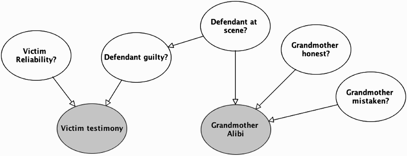
A BN graph for our legal example is depicted in Figure 1. It shows how the key pieces of evidence and crime-related hypotheses can be represented in a network of variables. In subsequent sections, we will show how this graph is generated from the case information, using an idiom-based approach.
Figure 1.
BN of crime example.
A node's NPT codifies the probability of each of its possible values, conditional on the values of its parent nodes. Any node without parents has an NPT that corresponds to its prior probability distribution. Once values for all the NPTs are given, the BN is fully ‘parameterized’. A parameterised BN can be used for a wide variety of probabilistic inferences. It can be used to calculate the probabilities of different hypotheses, given the available evidence, and also to predict the probable states of evidence variables not yet observed. Moreover, it can be used to answer various ‘what-if’ questions – such as the probability of attaining specific evidence if one supposes that a certain hypothesis is true (or false); and the probability of a crime hypothesis if one supposes that an evidential test turns out positive (or negative).
2.1.Markov condition
The defining property of a BN is that its variables satisfy the Markov condition (see Pearl 1988). Informally, this states that any variable in the BN graph is independent of all other variables (except its descendants) conditional on its parents. The Markov condition allows the joint probability distribution (of the variables in the BN) to be factorised in a more efficient and computationally tractable way, by taking advantage of the conditional independencies in the BN. This can greatly simplify probabilistic inferences and Bayesian updating. It allows for an encapsulated representation of a probability model without the need to store the full probability distribution across all variables. This is particularly important for large-scale networks, and affords great savings in storage and more efficient inference.
2.2.Bayesian updating and likelihood ratios
In essence, BNs generalise the principles of Bayesian reasoning to sets of interconnected variables. Central to Bayesian reasoning is the role of likelihood ratios to quantify the strength of evidence for (or against) a hypothesis, and the use of Bayes’ rule to update one's belief in a hypothesis, given new evidence. We will give a brief review of these concepts, showing how they are fundamental to the construction and use of BNs. Consider a simple two-variable network, where there is a directed link from a hypothesis (H) to an item of evidence (E), as shown in Figure 2. In this generic example, both the hypothesis and evidence variables are binary-valued (either true or false).
Figure 2.
Basic BN with two variables.
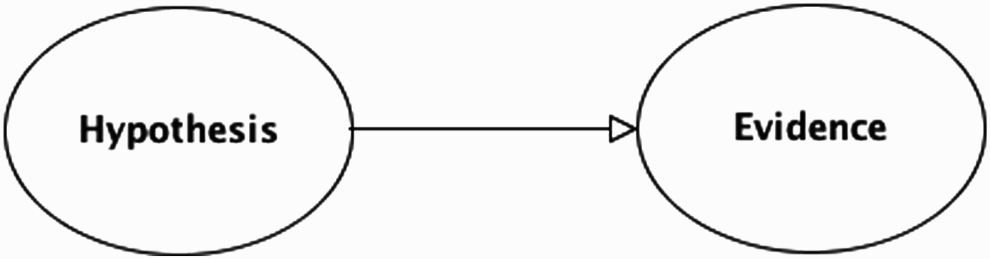
The link from H to E represents the assumption that the probability of the evidence depends on the truth status of the hypothesis – more precisely, that the probability of the evidence, given that the hypothesis is true, P(E| H), is different to (either greater or less than) the probability of the evidence, given that the hypothesis is false,
As well as quantifying the strength of the link between hypothesis and evidence, the LR dictates how much one should update one's beliefs in H, given new evidence E. This is achieved via Bayes’ rule, which is a basic theorem of the probability calculus. Bayes’ rule provides a formal procedure for moving from one's prior belief in H (without evidence E), to a posterior belief (with new evidence E). For simplicity, we will use the odds version of Bayes’ rule here:
In sum, Bayes’ rule tells us how to update our prior belief in the hypothesis, given new evidence. In the simple case of a BN with only two variables, a directed link from hypothesis to evidence represents a probabilistic relation that is quantified by the likelihood ratio. The NPTs for the hypothesis and evidence nodes gives a full parameterisation of the BN, and allows one to answer a range of probabilistic queries. For example, before finding out about the evidence E, we can calculate the probability of the evidence being true; and once we find out the status of the evidence, we can then update our probability for the hypothesis. We will illustrate the process of the BN computation in a worked example below.
3.The idiom-based approach
BNs have been successfully applied to a variety of real-world domains (see Pourret, Naim and Marcot 2008). They have also made inroads into forensic applications, most typically with regard to DNA evidence (Dawid and Evett 1997; Taroni et al. 2006). Two major problems arise when applying the standard BN approach to legal inference: (i) dealing with large numbers of variables; (ii) the lack of principled guidelines for constructing appropriate BN models. These two problems are tackled by adopting an idiom-based approach (Neil et al. 2000; Fenton et al. 2012).
The central idea behind the idiom-based approach is that large-scale inferential problems can be decomposed into a set of manageable components, each of which corresponds to a common inference schema. These schemas are termed idioms, and correspond to the basic building blocks that can be combined and reused to model complex multi-variable problems. The idioms themselves are generic, but they can be used to generate case-specific networks that retain the key inferential structure. Applied to the legal context, these idioms are tailored to the constraints and demands of legal enquiry – for example, focusing on questions of motive, means and opportunity, and issues of witness testimony and reliability. Most of these idioms are based on representations of causal processes that operate in a typical legal case. These include events and processes that occur prior, during and subsequent to the crime, and involve the behaviours of a range of agents such as the perpetrator, victim, witnesses, investigators, lawyers etc. Every crime case will involve a unique configuration of particular details, but the idiom-based approach allows us to apply generic inference patterns, and thus draw principled inferences. In the following sections, we will introduce some of the key legal idioms (see Fenton et al. 2012, for a fuller account) and apply them to our legal example.
3.1.Evidence idiom
This is the most basic idiom, and involves the relation between a hypothesis and an item of evidence. We have already introduced this generic model in the section above. In the legal context, a typical hypothesis would be a proposition relevant to the case, either a legal proposition that needs to be proved, such as whether the accused committed the crime in question, or a peripheral proposition that is relevant to the ultimate proposition, such as motive or opportunity. The evidence is typically an observation statement or report presented in court (or during the investigation), such as a witness testimony or a report from an expert. A directed link from the hypothesis to the evidence represents the causal process whereby the hypothesis generates the evidence.
To illustrate with our legal example: one critical hypothesis is the proposition that the suspect committed the robbery (which is either true or false). This proposition, if true, is a potential cause of the identification evidence given by the victim. In probabilistic terms, the truth of this hypothesis would raise the probability of a positive ID report, whereas the falsity of this hypothesis would lower the probability of a positive ID report. Conversely, (via Bayes’ rule), a positive ID report raises the probability that the suspect committed the crime, and a negative ID report lowers the probability of the suspect having committed the crime. Note that the probabilistic inferences can run both from causes to effects, and from effects to causes, but the BN representation captures the presumed causal direction in the world: hypothesis (cause) → evidence (effect).
The simple example of the evidence idiom is depicted in Figure 3. To see how Bayesian updating works in this case, we will use some hypothetical probabilities. Suppose that one's prior probability that the suspect committed the crime is 1/100. (This might be justified on the assumption that there are 99 other youths in the area that could have committed the crime). This prior probability is shown in the NPT for the hypothesis node in Figure 3. Furthermore, suppose that the probability of the minicab driver identifying the suspect, given that the suspect did commit the crime, P(E|H), is 0.9, whereas the probability of the minicab driver identifying the suspect, given that the suspect did not commit the crime,
Figure 3.
The evidence idiom applied to the ID report in the legal example (with NPTs below each node).
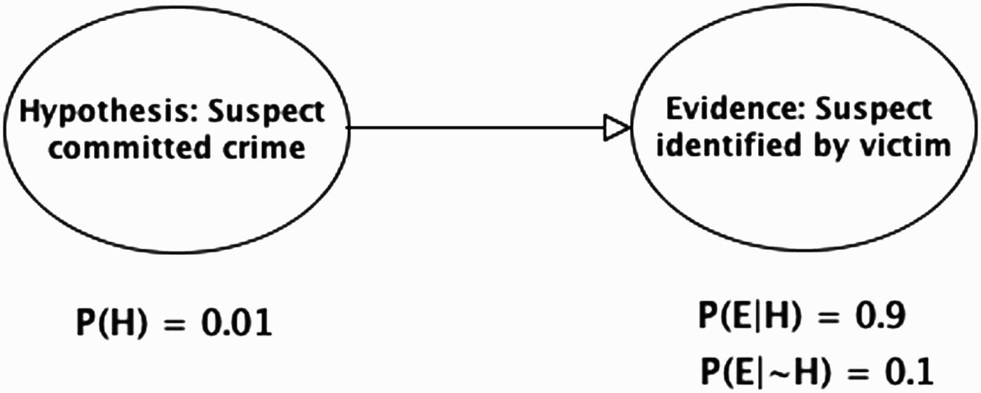
Figure 4.
Updated BN when victim provides a positive ID of the suspect.
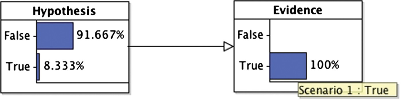
This example highlights the fact that a positive ID is not conclusive evidence that the suspect is guilty (far from it) – and that one's belief in this proposition depends on one's prior beliefs as well as the likelihood ratio for the evidence. A crucial component of the likelihood ratio is the probability of getting the evidence even if the suspect is not guilty. In the simple two-variable BN model, alternative possible causes of a positive ID are not explicitly represented. This is restrictive because there might be several distinct factors that can lead to a false positive ID, and it might be important to distinguish between these alternative causes (as we shall see below). Moreover, there might be other evidence in the case that is relevant to only one of these alternative causes. To overcome these issues, it is useful to represent alternative causes explicitly, as separate nodes in the BN.
3.2.Evidence reliability idiom
The evidence–reliability idiom introduces an additional node to represent the reliability of the evidence statement. It makes it explicit that the evidence report is fallible, and that there are other causal factors that can influence the production of the evidence report, and indeed can lead to a positive report even when the hypothesis is false (see Bovens and Hartmann 2003, for a similar BN approach to modelling reliability in epistemology and philosophy of science, and Friedman 1987, for BN-like approach in legal contexts).
The evidence–reliability idiom captures the fact that any measuring process is imperfect. The reliability node moderates the extent to which the evidence report produced by the measuring process is an accurate reflection of the true status of the hypothesis. In the limiting case, with a fully reliable measuring process, the status of the hypothesis guarantees the status of the evidence report, and vice-versa. However, real measuring devices will always have some degree of fallibility. This is particularly true when the measuring device is human testimony. Aside from being notoriously fallible, the case of human testimony introduces additional complexity because human witnesses are sometimes motivated to deceive. (This latter situation is discussed below in an extension of the evidence–reliability idiom.)
To start with, we will focus on the simple case where the reliability of the evidence report is assumed to be causally independent of the target hypothesis. This gives us a BN structure with two parent (causal) nodes for the evidence report (see Figure 5). This model represents situations where there are two (non-exclusive) causal factors that can contribute to the evidence report. This can be applied to the legal example above. There are two potential causes of the victim's testimony: the suspect was indeed the person who threatened the victim (the crime hypothesis), or the victim was mistaken in their identification (the reliability hypothesis). Although these two causes furnish alternative explanations they are not mutually exclusive. It is possible that the suspect threatened the victim and that the victim's testimony is unreliable. In this BN model, we assume that the causal variables are (unconditionally) independent – that prior to the testimony evidence, the probability of the victim being reliable is independent of whether or not the suspect committed the crime (this seems a reasonable assumption in this situation). However, once the testimony evidence is given, the two cause variables become conditionally dependent – they compete to explain the evidence.
Figure 5.
Evidence–reliability idiom applied to legal example (R=reliability ).
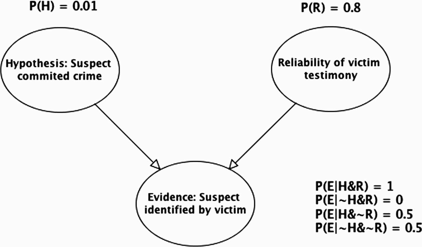
To calculate the impact of the testimony evidence on the two potential explanations, we need to know (or estimate) their prior probabilities, and the conditional probabilities of the testimony evidence, given all the possible states of the causes (parents). In the legal example, we make the simplifying assumption that the victim is either reliable or not (i.e. the variable Reliable is either true or false). Thus, there are four possible states: (i) suspect did commit crime and victim reliable (H&R), (ii) suspect did not commit crime and victim reliable (∼H&R), (iii) suspect did commit crime and victim not reliable (H&∼R), (iv) suspect did not commit crime and victim not reliable (
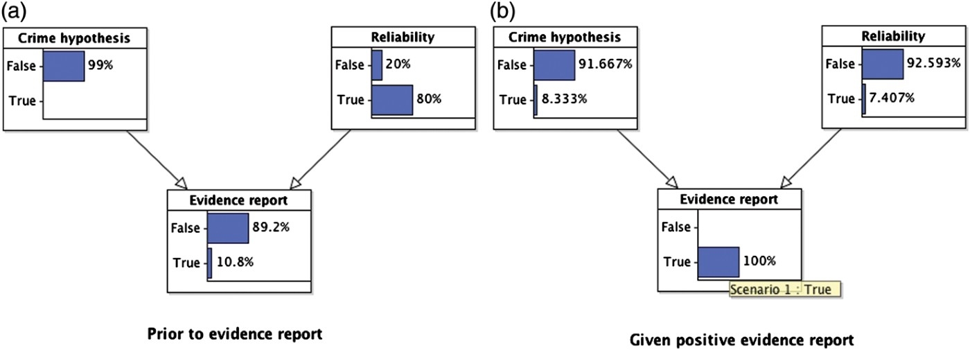
To complete the parameterisation of the BN model, we need to assign priors for the hypothesis that the suspect committed the crime (e.g. 1/100 as above), and for the witness being reliable. We will suppose that the prior probability for the victim's reliability is=8/10. Given the fully specified BN model (see Figure 5), we can compute various probabilities. In the absence of any evidence report, and using just the prior probability information, the probability of receiving a positive ID report is 10.8% (see Figure 6(a)). Once a positive evidence report is given, the probability of the suspect being guilty rises to 8.33%, but the probability that the witness is reliable drops to 7.41% (see Figure 6(b)). This captures the fact that the unreliability of the witness is a more plausible explanation for the positive ID report than the suspect being guilty.
Figure 6.
Evidence–reliability idiom applied to the legal example with witness testimony.
We can also answer various ‘what-if’ questions. For example, suppose that we knew that the witness was unreliable. This would reduce the probability that the suspect is guilty back to the value it took prior to the evidence report because the evidence report no longer gives any information about whether the suspect committed the crime (see Figure 7(a)). On the other hand, suppose that we knew for sure that the witness was reliable. Then the probability that the suspect is guilty increases to one, because the witness is fully reliable (see Figure 7(b)).
Figure 7.
Two ‘what-if’ scenarios showing ‘explaining away’ reasoning.
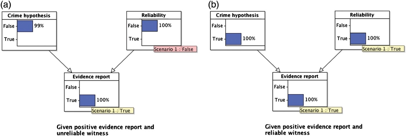
As noted above, a critical feature of this BN model is that although, prior to knowing the status of the evidence report, the two hypotheses (suspect guilty or witness unreliable) are independent, once we know the status of the report, the two hypotheses become dependent, and compete to explain the evidence. This pattern of inference is known as ‘explaining away’ and is naturally captured within the BN framework (and is less readily modelled by other formal systems). It is ubiquitous in the legal context, because it provides the template for the claims and rebuttals characteristic of much of the evidence presented in court.
Although, we have illustrated the evidence–reliability idiom with an example of the eyewitness testimony, the idiom applies equally to evidence generated by any type of measurement procedure (e.g. CCTV, DNA and other forensic evidence). However, even where the measuring procedure seems more ‘objective’ than human testimony, the interpretation and presentation of an evidential report will typically (always?) involve some element of human judgment, and is thus susceptible to many of the same qualifications as human testimony. For example, the statement of a DNA or fingerprint match ultimately relies on an expert judgment. In some situations, it might be important to distinguish between reliabilities of the measurement process itself and the human expert, even for the same piece of evidence. For instance, the reliability of the process of generating a DNA profile as well as the reliability of the process of interpreting the profiles (see Fenton et al. 2012 for more details).
3.3.Opportunity and motive idioms
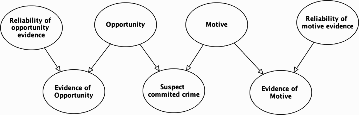
Opportunity and motive are typically considered to be important precursors to most crimes. Thus, for crimes such as assault, rape, burglary, and in most cases of murder, opportunity is a pre-requisite for someone to be found guilty. If the defendant was not at the crime scene, then they could not have committed the crime. While it is not crucial to prove the motive in order to find a defendant guilty, it too is often a key part of the case against the defendant. From a BN perspective, what is distinctive about both opportunity and motive is that they are causal pre-conditions for guilt, and thus need to be modelled as parent variables to the main crime hypothesis. This is shown in Figure 8. It is also important to separate out hypotheses about motive or opportunity, from the evidence reported to support (or undermine) these hypotheses. And this evidence in turn can be subject to questions of reliability. These relations are depicted by the evidence and reliability nodes in the Figure 8.
Figure 8.
BN with opportunity and motive nodes.
In our legal example, the minicab driver's testimony was directly relevant to the main hypothesis that the suspect committed the crime, whereas the grandmother's testimony was about opportunity. This corresponds to the legal distinction between direct and circumstantial evidence. We will illustrate the key role of opportunity evidence when we discuss the legal example in more detail below.
3.4.Reliability unpacked (into sensitivity, objectivity and veracity)
So far we have introduced a single variable, reliability, to cover the possibility that an evidence source is inaccurate. However, the concept of reliability is ambiguous, and there are several different ways in which a source of evidence can be unreliable. Schum (1994) distinguishes three separate components of reliability: (i) observational sensitivity (accuracy), (ii) objectivity, and (iii) veracity.22
The notion of observational sensitivity corresponds most closely to the use of reliability in the section above. It applies both to human and mechanical measurement devices, and concerns the degree to which the detector is able to measure the status of the hypothesis (and distinguish this from the noise inherent in the measurement process). In the case of human testimony, observational sensitivity is often dependent on factors such as the viewing conditions, the perceptual capabilities of the observer, the expertise of the observer etc. In our legal example, this might correspond to the poorly lit street, the hoodie worn by the assailant, and the disorientation of the victim during the crime. These are factors that might affect how well the witness encoded the crime incident, but there will also be various factors that might affect the victim's recall of this information when he has to identify the culprit in the ID parade.
Schum's notion of objectivity refers to the belief formation process (rather than just sensory perception). What distinguishes it from observational sensitivity is the possibility of a systematic bias in the belief formation process of the witness, independent of how sensitive is their perceptual apparatus. Thus, a witness might over-interpret the sensory information he receives due to strong prior expectations, or some kind of response bias. It is important to note that this lack of objectivity is not deceitful – it is a function of the belief formation process of the witness, and the influence of the context. For example, a witness at an ID parade might have an expectation that the culprit must be in the line-up, and thus develop a response bias to make a positive ID, even when he is not sure. This is an honest mistake (on the part of the witness), but one that can be encouraged by the manner in which the ID parade is conducted (e.g. sequential versus simultaneous presentation, instructions to the witness, the make-up of the line-up, see Wells ref). Similarly, an expert witness can be susceptible to objectivity bias when making a forensic judgment due to other available knowledge about the case. For example, fingerprint experts have been shown to be biased by external information that is not strictly relevant to their match judgment (Dror and Charlton 2006). Here again the bias is not wilful, but due to the belief/decision-making process and the effect of context.
The notion of veracity is perhaps the most distinctive issue raised by witness testimony, especially when the witness has a stake in the outcome of the legal process. The suspicion that a witness might be lying is especially pertinent when the suspect, or someone partial to the suspect, is providing testimony. This explains why alibi evidence from a close relative or friend is generally treated with great caution, if not outright disbelief (Gooderson 1977). The alibi provider in such cases has a strong motivation to lie in order to protect the suspect. The question of veracity is typically independent of the other two sources of inaccuracy. A witness can be honest (or dishonest) irrespective of whether they are observationally sensitive or objective.
A more comprehensive approach to modelling reliability takes these three separate components of reliability into account. In the fuller BN idiom, each component is represented as a separate parent node of the evidence report (see Figure 9). Along with the hypothesis that is the subject of the evidence report, each of these variables is a potential causal factor relevant to the evidence report. This does not mean that reliability always needs to be unpacked into all three variables, sometimes it will suffice to work with just one or two of these variables.
Figure 9.
BN idiom for three components of reliability: observational sensitivity, objectivity and veracity. Note in this model the evidence report concerns the question of opportunity.
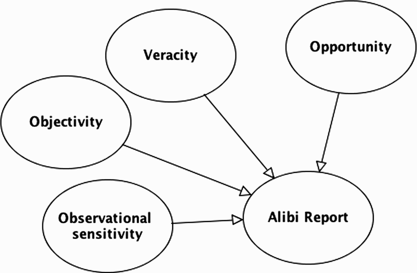
Representing the separate components of reliability allows us to clarify how different pieces of evidence might impact on different aspects of a witness's reliability. For example, in court a witness report might be countered on the grounds that the witness is dishonest or has poor observational sensitivity (or both). Each of these issues might require a different kind of evidence. Thus, evidence of dishonesty might come from a poor character reference whereas evidence of observational insensitivity might come from eye-test results. Analysing reliability into subcomponents also allows us to capture additional probabilistic links that might be disguised at a coarser level of representation. This is particularly apposite when a witness's honesty is in question.
3.5.Alibi idiom
A distinctive feature of veracity is that it will sometimes depend on the truth status of the crime hypothesis; this is especially likely when someone partial to the defendant provides the testimony. The classic example of this is alibi testimony. If true, an alibi absolves the suspect of guilt, because it rules out the opportunity for committing the crime (here we are ignoring crimes that they can commit remotely). This is captured in the NPT for guilt, where the probability of committing some crimes, given no opportunity, would be zero, see above). However, when the suspect, or a close friend or relative of the suspect, supplies the alibi, it is natural to suppose that they have a strong motivation to lie to protect themselves. In addition, one might suppose that this inclination to lie is greater if the suspect is in fact guilty rather than innocent. (This is not always a valid supposition to make, but seems reasonable as a default assumption, see below for more discussion).
Because of this distinctive feature, we term this the alibi idiom – although it is not restricted to alibi evidence, and can apply to any kind of witness testimony. The key novelty is that there is a potential link from the crime hypothesis to the reliability (veracity) of the testimony report. This is depicted in Figure 10, where there is a direct link from the guilty hypothesis (‘suspect committed crime’ node) to the node representing the veracity of the witness. This link corresponds to the assumption that the witness is more likely to lie in their testimony if the defendant is guilty rather than innocent.
Figure 10.
BN of alibi idiom, which incorporates the link from suspect guilt to witness veracity. This will be very common when the suspect provides his own alibi.
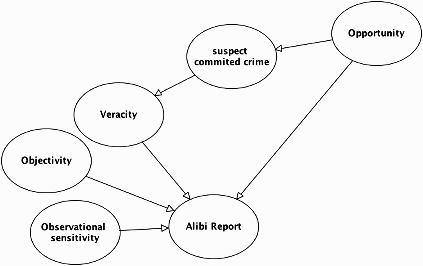
There is an important qualification here – the viability of a link from the crime hypothesis to veracity will depend on the knowledge or beliefs of the witness. When the alibi witness is the suspect, we can assume that the suspect knows whether or not he is guilty, and this justifies the link from guilt to veracity. However, in cases where the alibi witness does not know whether or not the suspect is guilty, this link is less plausible. It will depend on other knowledge possessed by the witness. On one hand, imagine an alibi witness who is partial to the suspect, but does not know whether the suspect is guilty, and no reason to believe either way. In this situation, the link from guilt to veracity seems implausible: whether or not the witness decides to lie is independent of whether the suspect is guilty. On the other hand, consider an alibi witness who does not know for sure if the suspect is guilty, but has suspicions, based on evidence he has observed, that the suspect is indeed guilty. In this case, the veracity of the witness might still depend on whether the suspect is guilty. There is an indirect link from guilt to veracity via the evidence observed by the witness (see Figure 10).
An important consequence of the alibi idiom is that the discovery that an alibi witness has presented a false alibi can have a double-effect on judgments about the probability that the suspect is guilty. For example, suppose that a suspect in an assault case presents an alibi. If the police uncover independent evidence that the suspect was at the crime scene (e.g. via CCTV evidence), then not only is the suspect's alibi undermined, but the police also know that the suspect is lying. This is doubly incriminating – the suspect has been placed at the crime scene (and has opportunity), but has also been caught out as giving a false alibi. It is natural to take this lie as further evidence of his guilt. Indeed, this is exactly the ‘adverse’ inference that judges warn jurors about (see above). This does not make it an illegitimate inference, but marks it out as an inference that requires careful consideration (effectively requiring that jurors are sure about the assumptions they are making). The alibi idiom allows us to capture this important pattern of inference (see Lagnado 2011, for further details and BN models of different alibi contexts).
3.6.Combining the idioms
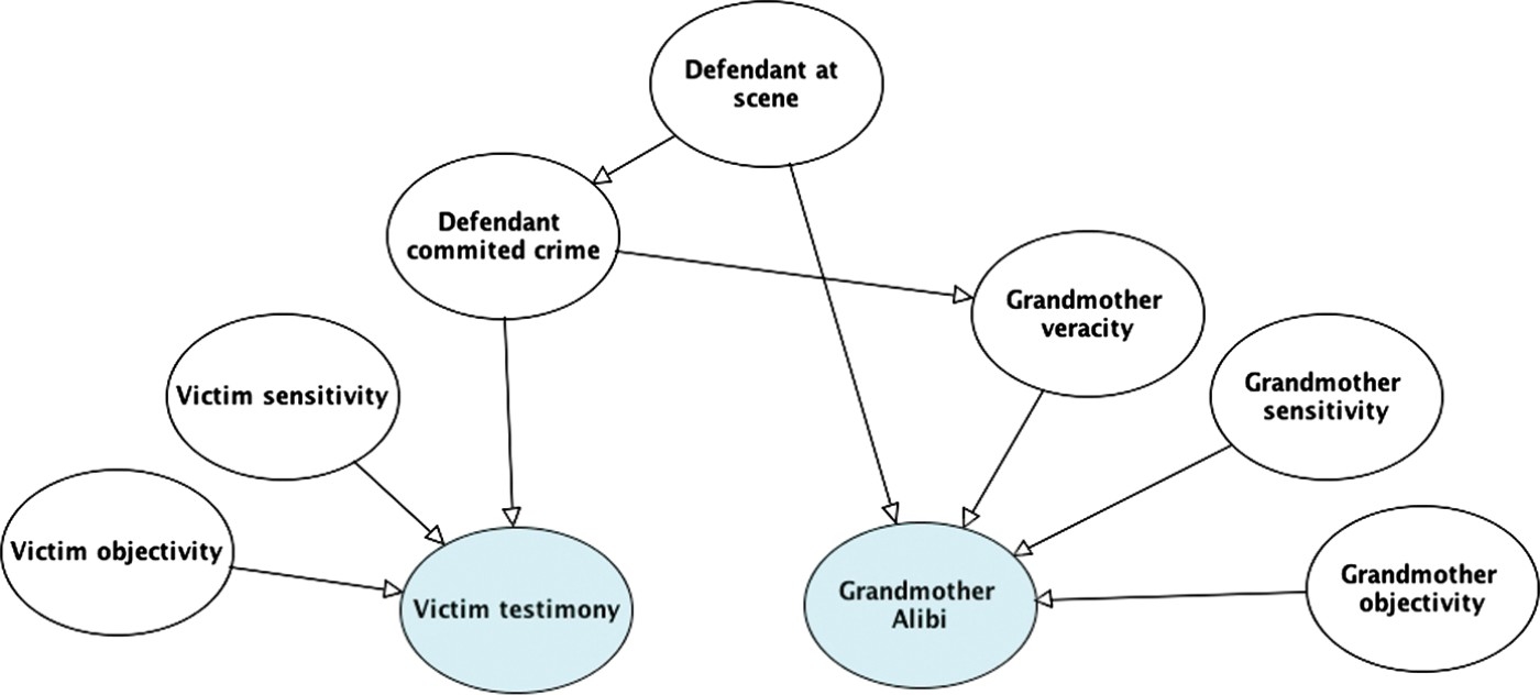
A key strength of the idiom-based approach is that a small set of idioms can be combined and reused to generate a model of the case and to support inferences about the likely explanations for the evidence. Our legal example can be modelled by using the evidence–reliability, alibi and opportunity idioms. The central crime hypothesis is whether or not the suspect committed the crime. There are two main pieces of evidence: the victim's testimonial report that identified the defendant as the perpetrator, and the grandmother's alibi statement that the defendant was with her at the time of the crime, and therefore could not have committed the robbery. The victim's testimony can be modelled using the evidence–reliability idiom, and further decomposed with reliability components of observational sensitivity, objectivity and veracity. The grandmother's testimony concerns opportunity, and the reliability of this testimony can also be decomposed into the same three components. In addition, due to the partiality of the grandmother, there is an extra possible link from the crime hypothesis to the veracity of her statement. This corresponds to the alibi idiom. The full BN model is shown in Figure 11.
Figure 11.
BN model for legal example using the idiom-based approach.
This model can be developed in several ways. In particular, there is additional evidence to consider arising from the grandmother's flawed testimony. Recall that under cross-examination, the grandmother's testimony was shown to be inconsistent: she failed to recall the precise night in question, and was unclear about the date or day of week. This could be evidence of her lack of sensitivity, objectivity or veracity, or some combination of all three (see Figure 12). How the jury interpreted this inconsistency was crucial to their final decision (as argued by the court of appeal). In stark terms, the jury seemed to believe that she was lying to protect her grandson rather than suffering from memory failure.
Figure 12.
BN for legal example with evidence from grandmother's cross-examination added.
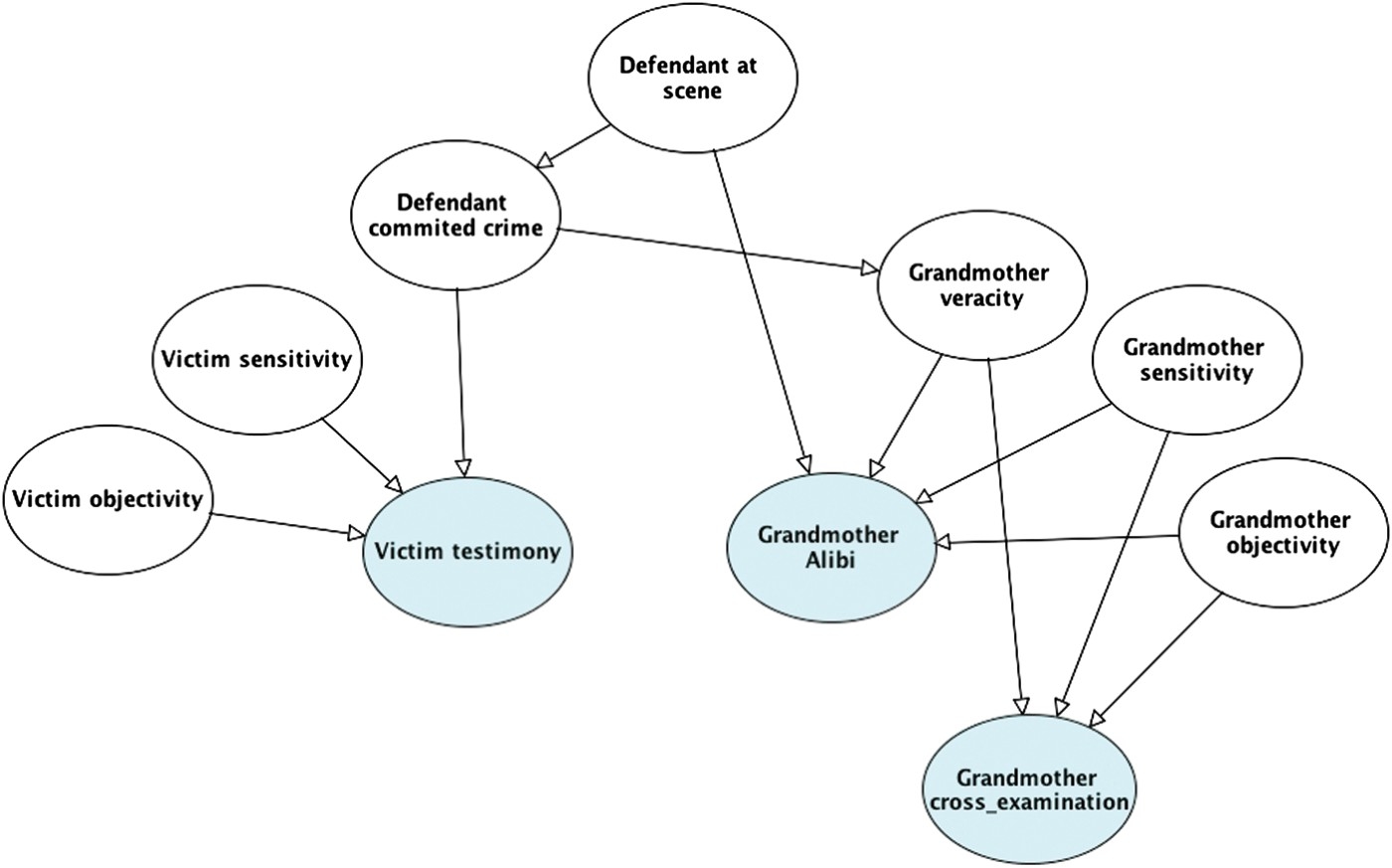
The alibi idiom highlights a further complication. Suppose that the grandmother was indeed lying to protect her grandson. This discovery is sufficient to undermine the alibi, but does not imply that the suspect is guilty. Another important question is whether the grandmother knows if her grandson is guilty. (And thus whether there is a link from guilt to veracity in the BN). This makes a difference to what inferences we can draw from her false alibi. If she does not know whether or not he is guilty, her lie is not diagnostic of guilt because the lie does not depend on whether or not he is guilty. However, if she does know, and we assume that she is more likely to lie if he is guilty than if he is innocent, then her lying is diagnostic of guilt.
4.Empirical study of alibi testimony
To explore whether people's intuitive judgments conform to the BN model of alibi testimony presented in this paper, we constructed a short study based on the legal case in R v Pemberton (1994). The study examined the impact of a discredited alibi on people's judgments of guilt, and in particular whether people draw different inferences according to whether they believe that a false alibi is due to a genuine mistake or an intentional lie. To investigate this question, two separate conditions were constructed: Alibi 1, where the false testimony was presented as a memory error, and Alibi 2, where it was presented as an intentional lie. Based on the BN analysis of the alibi testimony given above, we predicted that in Alibi 1 people would discount the alibi testimony, but not increase their belief in the suspect's guilt – the false alibi was sufficiently explained by the possibility of the memory error. In contrast, in Alibi 2, we predicted that the discredit of the alibi would increase participants’ judgments of guilt, because they believed that the grandmother was lying to protect her grandson (and that she was more likely to lie if he was guilty).
4.1.Method
The experiment was conducted online with 44 participants from the general population.33 They were instructed to imagine that they were jurors in a criminal case. They were split into two conditions: Alibi 1 or Alibi 2. In both conditions, participants received (i) the same background information about the case, and then (ii) the same alibi testimony from the grandmother (see Table 1 for summary). They then received information about the cross-examination of the grandmother (iii). In Alibi 1, this highlighted the fact that the grandmother was confused about the exact date; in Alibi 2, it was revealed that she had a train ticket showing she was not at home on the night in question. Participants made probability judgments about the suspect's guilt after each piece of information, using a rating scale from
Table 1.
Summary of information presented in alibi conditions.
| Alibi condition 1 | Alibi condition 2 | |
| Background | A minicab driver collected a man from Tooting. On the way, the passenger gave directions to an address in Brixton but the minicab driver refused and told the passenger to get out. The passenger then pulled out a knife, took ignition keys and money from the coin box. He disappeared between two blocks of flats. The police arrived and searched the area without success. Three hours later, the cab driver saw the man he believed robbed him come out of the flats. The cab driver followed him a little way until he disappeared | |
| The suspect was collected from home fully clothed and lying in bed. At a subsequent identification parade, the cab driver picked out the suspect as the robber. When interviewed by the police after the parade, the suspect denied robbery, claiming that it was just mistaken identity, and that he had not been out that night because he was sick | ||
| Alibi | His grandmother, with whom he lived, gave evidence that he did not go out on the night in question | |
| Discredit of alibi | Under cross-examination, the grandmother could not precisely remember the night in question. The prosecution lawyer claimed that the grandmother was lying in her alibi | Under cross-examination, the grand-mother could not precisely remember the night in question. A used return train ticket booked for the night in question was found suggesting that the grandmother was in Kent. The prosecution lawyer claimed that the grandmother was lying in her alibi |
| Additional rating questions | (a) Do you think that the grandmother would have lied if she knew that her grandson HAD committed the robbery? | |
| (b) Do you think that the grandmother would have lied if she knew that her grandson HAD NOT committed the robbery? | ||
| How much do you believe the alibi? | ||
4.2.Results and discussion
The mean ratings for each stage (i–iii) are shown in Figure 13. We analysed the two conditions separately. For Alibi 1, alibi judgments were lower than baseline (t(21)=2.72, p=0.013) and discredit judgments (t(21)=3.00, p=0.007), but there was no difference between baseline and discredit judgments (t(21)=0.84, p=0.407). For Alibi 2, alibi judgments were no different to baseline (t(21)=0.58, p=0.566), but were lower than discredit judgments (t(21)=5.23, p=0.001). Of particular note, discredit judgments were higher than baseline judgments (t(21)=3.40, p=0.003).
Figure 13.
Mean probability of guilt ratings for the three stages of information; (i) baseline, (ii) alibi, (iii) discredit of alibi. Alibi 1 condition on the left-hand side, Alibi 2 condition on the right-hand side.
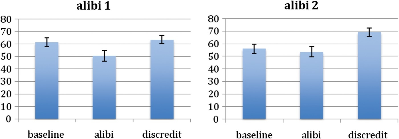
The key finding is that in Alibi 1, the alibi discredit returned guilty ratings to the baseline level (false alibi explained as an innocent mistake), whereas in Alibi 2, the alibi discredit actually increased ratings above the baseline (false alibi explained as intentional deception). This interpretation is supported by the other judgments taken at the end of the task. In both conditions, participants judged that the grandmother was more likely to lie if she knew that her grandson was guilty (m=63.25) rather than if she knew he was innocent (m=32.20), (t(43)=5.15, p=0.001); however, the believability of the alibi was rated more highly in Alibi 1 (m=40.6) than Alibi 2 (m=28.7), (t(21)=2.56, p=0.014).
In sum, these results confirm the predictions based on the BN analysis given above. In Alibi 2, people draw an adverse inference from the false alibi, because their model of the evidence includes a link from guilt to veracity (see Figure 11), and they infer that the grandmother is lying in her alibi. In Alibi 1, people do not draw this adverse inference; they consider that the false alibi might have arisen from a genuine error.
5.Discussion
The idiom-based approach is primarily presented as a normative and prescriptive framework for reasoning about evidence. We have outlined some of the key idioms that apply to legal enquiry, and shown how they are based on rigorous patterns of probabilistic inference. A secondary goal of this paper is to argue that the idiom-based approach, and in particular its reliance on causal idioms, gives a guide to how people actually reason with complex bodies of evidence. We have provided a brief study to support this claim (see also Lagnado 2011), but clearly there is much more empirical work still to be done. However, we believe that the plausibility of the idiom-based approach as a cognitive model is also supported by earlier empirical studies in juror decision-making, especially those conducted by proponents of the story model (Pennington and Hastie 1986, 1992).
The story model argues that people evaluate legal evidence by constructing causal narratives that explain the evidence. These narratives are built up from people's causal understanding of how things typically happen, and in particular how protagonists act on the basis of psychological states such as intentions. It also emphasises that smaller causal schemas (scripts and episodes) are pieced together to construct an overarching story, and that this story dictates people's subsequent decisions. In these respects, the idiom-based approach is very similar to the story model, especially in its emphasis on reusable and combinable causal schemas. These similarities mean that the wealth of empirical data gathered by the story model in support of the role of causal representations can also be taken to confirm the idiom-based approach.
However, there are important differences between the two accounts. The idiom-based approach is rooted in the BN framework, with idioms corresponding to the qualitative (graphical) component of this framework. This gives it both a normative and computational basis in probabilistic reasoning. In contrast, the story model explicitly disavows the use of probabilistic inference, and has no clear formal basis or link to normative theories of evidence evaluation. We believe that the story model's rejection of probabilistic reasoning is premature, and partly due to a failure to distinguish the qualitative and quantitative aspects of probabilistic approaches. Our proposed account focuses on qualitative aspects of Bayesian reasoning. In addition, there are a variety of qualitative reasoning systems (Druzdzel 1996; Parsons 2001; Keppens 2007) that capture sound probabilistic inference without requiring fully Bayesian computations over precise probability assignments.
The relation between the idiom-based approach and the story model merits further exploration, both with regard to integrating the notions of causal idioms and schemas, and clarifying the role of probabilistic reasoning. This is particularly pertinent in light of recent movements in cognitive science that apply more sophisticated Bayesian models to cognition (Krynski and Tenenbaum 2007; Oaksford and Chater 2007, 2010; Griffiths, Kemp and Tenenbaum 2008). Of particular relevance here is research that gives a Bayesian account of argumentation (Hahn and Oaksford 2007; Harris and Hahn 2009; Corner et al. 2011; Jarvstad and Hahn 2011; see also Hahn, Oaksford and Harris 2012). This latter work dovetails with the claims made in this paper, and potentially provides an overarching framework for argument evaluation in general. In this light, the BN framework, combined with causal idioms, seems an apposite framework to revisit earlier models of juror reasoning.
6.Conclusions
We have presented an idiom-based framework for understanding evidential reasoning. In particular, we have focused on modelling witness and alibi testimony, and how these interrelate with other pieces of evidence. We believe that the idiom-based framework provides a rigorous foundation for modelling and assessing legal arguments,44 and that it serves as a guiding framework for key aspects of human evidential reasoning. For example, recall the legal case where the grandmother's alibi testimony was discredited. In the actual appeal of this case, it was ruled that the conviction was unsafe because the judge had not given appropriate instructions to the jury on what conclusions could legitimately be drawn from a false alibi. Our Bayesian analysis clarifies the key assumptions and inferences in such a case. The approach also has the potential to be developed into a principled tool for structuring our thinking about complex legal cases. Thus, it might serve as a useful corrective in those cases where human reasoning does depart from the normative model.
Notes
1 These conditional probabilities do not need to equal 0.5; there could be contexts where an unreliable source is more likely to give a positive rather than a negative report (or vice-versa). The key point is that they are equal:
2 A similar approach is adopted by Friedman (1987), also using inference networks.
3 The current experiment has a relatively small sample size. However, very similar findings have been replicated with larger sample sizes and across several variations of alibi evidence (see Lagnado 2011, 2012).
4 We lack the space to discuss other formal approaches to legal argument (Walton 2008). For comparison between the BN approach and other theories of argumentation, see Fenton et al. (2012). One of the main differences is that argumentation approaches have typically avoided the use of probability theory and Bayesian reasoning to model uncertainty.
Acknowledgements
David Lagnado is supported by ESRC grant (RES-062-33-0004). We thank Jamie Tollentino for help with constructing the materials and running the experiment.
References
1 | Bovens, L. and Hartmann, S. (2003) . Bayesian Epistemology, Oxford: Oxford University Press. |
2 | Corner, A., Hahn, U. and Oaksford, M. (2011) . ‘The Psychological Mechanism of the Slippery Slope Argument’. Journal of Memory and Language, 64: : 133–152. (doi:10.1016/j.jml.2010.10.002) |
3 | Crown Court Benchbook (2010), http://www.judiciary.gov.uk/publications-and-reports/judicial-college/ Judicial College: Judicial Studies Board. |
4 | Dawid, A. P. and Evett, I. W. (1997) . ‘Using a Graphical Model to Assist the Evaluation of Complicated Patterns of Evidence’. Journal of Forensic Sciences, 42: : 226–231. |
5 | Dennis, I. (2007) . The Law of Evidence, 3, London: Thomson Sweet & Maxwell. |
6 | Dror, I. E. and Charlton, D. (2006) . ‘Why Experts Make Errors’. Journal of Forensic Identification, 56: (4): 600–616. |
7 | Druzdzel, M. (1996) . ‘Qualitative Verbal Explanations in Bayesian Belief Networks’. Artificial Intelligence and Simulation of Behaviour Quarterly, 94: : 43–54. |
8 | Edwards, W. (1991) . ‘Influence Diagrams, Bayesian Imperialism, and the Collins Case: An Appeal to Reason’. Cardozo Law Review, 13: : 1025–1079. |
9 | Fenton, N. and Neil, M. (2011) . ‘Avoiding Legal Fallacies in Practice Using Bayesian Networks’. Australian Journal of Legal Philosophy, 36: : 114–150. |
10 | Fenton, N., Neil, M. and Lagnado, D. A. (2012) . ‘A General Structure for Legal Arguments about Evidence using Bayesian Networks’ Cognitive Science, in press. |
11 | Friedman, D. (1987) . ‘Route Analysis of Credibility and Hearsay’. Yale Law Journal, 96: (4): 667–742. (doi:10.2307/796360) |
12 | Gooderson, R. N. (1977) . Alibi, London: Heinemann Educational. |
13 | Griffiths, T. L., Kemp, C. and Tenenbaum, J. B. (2008) . “‘Bayesian Models of Cognition’”. In The Cambridge Handbook of Computational Cognitive Modelling, Edited by: Sun, R. New York: Cambridge University Press. |
14 | Hahn, U. and Oaksford, M. (2007) . ‘The Rationality of Informal Argumentation: A Bayesian Approach to Reasoning Fallacies’. Psychological Review, 114: : 704–732. (doi:10.1037/0033-295X.114.3.704) |
15 | Hahn, U., Oaksford, M. and Harris, A. (2012) . Rational Argument, Rational Inference. Argument and Computation In press. |
16 | Harris, A. J.L. and Hahn, U. (2009) . ‘Bayesian Rationality in Evaluating Multiple Testimonies: Incorporating the Role of Coherence’. Journal of Experimental Psychology: Learning, Memory, and Cognition, 35: : 1366–1372. (doi:10.1037/a0016567) |
17 | Hepler, A. B., Dawid, A. P. and Leucari, V. (2007) . ‘Object-Oriented Graphical Representations of Complex Patterns of Evidence’. Law, Probability & Risk, 6: : 275–293. (doi:10.1093/lpr/mgm005) |
18 | Jarvstad, A. and Hahn, U. (2011) . ‘Source Reliability and the Conjunction Fallacy’. Cognitive Science, 35: : 682–711. (doi:10.1111/j.1551-6709.2011.01170.x) |
19 | Kadane, J. B. and Schum, D. A. (1996) . A Probabilistic Analysis of the Sacco and Vanzetti Evidence, New York: John Wiley. |
20 | Keppens, J. ‘Towards Qualitative Approaches to Bayesian Evidential Reasoning’. Proceedings of the 11th International Conference on Artificial Intelligence and Law. pp. 17–25. |
21 | Krynski, T. R. and Tenenbaum, J. B. (2007) . ‘The Role of Causality in Judgment under Uncertainty’. Journal of Experimental Psychology: General, 136: : 430–450. (doi:10.1037/0096-3445.136.3.430) |
22 | Lagnado, D. A. (2011) . “‘Thinking about Evidence’”. In Evidence, Inference and Enquiry, Edited by: Dawid, P., Twining, W. and Vasilaki, M. Vol. 171: , 183–224. Oxford: Oxford University Press. Proceedings of the British Academy |
23 | Lagnado, D. A. (2012) . “‘Adverse Inferences about Alibi Evidence’”. Manuscript under preparation. |
24 | Lagnado, D. A. and Harvey, N. (2008) . ‘The Impact of Discredited Evidence’. Psychonomic Bulletin & Review, 15: : 1166–1173. (doi:10.3758/PBR.15.6.1166) |
25 | Neil, M., Fenton, N. and Nielsen, L. (2000) . ‘Building Large-Scale Bayesian Networks’. Knowledge Engineering Review, 15: : 257–284. (doi:10.1017/S0269888900003039) |
26 | Oaksford, M. and Chater, N. (2007) . Bayesian Rationality: The Probabilistic Approach to Human Reasoning, Oxford: Oxford University Press. |
27 | Oaksford, M. and Chater, N. (2010) . Cognition and Conditionals: Probability and Logic in Human Thinking, Oxford: Oxford University Press. |
28 | Parsons, S. (2001) . Qualitative Methods for Reasoning under Uncertainty, Cambridge, MA: MIT Press. |
29 | Pearl, J. (1988) . Probabilistic Reasoning in Intelligent Systems, Palo Alto, CA: Morgan Kaufmann. |
30 | Pennington, N. and Hastie, R. (1986) . ‘Evidence Evaluation in Complex Decision Making’. Journal of Personality and Social Psychology, 51: : 242–258. (doi:10.1037/0022-3514.51.2.242) |
31 | Pennington, N. and Hastie, R. (1992) . ‘Explaining the Evidence: Test of the Story Model for Juror Decision Making’. Journal of Personality and Social Psychology, 62: : 189–206. (doi:10.1037/0022-3514.62.2.189) |
32 | Pourret, O., Naim, P. and Marcot, B. (2008) . Bayesian Networks: A Practical Guide to Applications, Chichester: Wiley. |
33 | Robertson, B. and Vignaux, T. (1995) . Interpreting Evidence: Evaluating Forensic Science in the Courtroom, New York: John Wiley. |
34 | R. v Pemberton (1994), 99 Cr. App. R. 228. CA. |
35 | Schum, D. A. (1994) . The Evidential Foundations of Probabilistic Reasoning, Northwestern University Press. |
36 | Taroni, F., Aitken, C., Garbolino, P. and Biedermann, A. (2006) . Bayesian Networks and Probabilistic Inference in Forensic Science, Chichester: John Wiley. |
37 | Tillers, P. and Green, E. (1988) . Probability and Inference in the Law of Evidence: The Uses and Limits of Bayesianism, Dordrecht, Netherlands: Kluwer Academic Publishers. |
38 | Walton, D. (2008) . Witness Testimony Evidence: Argumentation, Artificial Intelligence, and Law, Cambridge: Cambridge University Press. |


