
Probabilistic abstract argumentation: an investigation with Boltzmann machines
Abstract
Probabilistic argumentation and neuro-argumentative systems offer new computational perspectives for the theory and applications of argumentation, but their principled construction involves two entangled problems. On the one hand, probabilistic argumentation aims at combining the quantitative uncertainty addressed by probability theory with the qualitative uncertainty of argumentation, but probabilistic dependences amongst arguments as well as learning are usually neglected. On the other hand, neuro-argumentative systems offer the opportunity to couple the computational advantages of learning and massive parallel computation from neural networks with argumentative reasoning and explanatory abilities, but the relation of probabilistic argumentation frameworks with these systems has been ignored so far. Towards the construction of neuro-argumentative systems based on probabilistic argumentation, we associate a model of abstract argumentation and the graphical model of Boltzmann machines (BMs) in order to (i) account for probabilistic abstract argumentation with possible and unknown probabilistic dependences amongst arguments, (ii) learn distributions of labellings from a set of cases and (iii) sample labellings according to the learned distribution. Experiments on domain independent artificial datasets show that argumentative BMs can be trained with conventional training procedures and compare well with conventional machines for generating labellings of arguments, with the assurance of generating grounded labellings – on demand.
1.Introduction
The combination of formal argumentation and probability theory to obtain formalisms catering for qualitative uncertainty as well as qualitative uncertainty has attracted much attention in the recent years, see, for example, Li et al. (2011), Thimm (2012), Hunter (2013), Sneyers et al. (2013) and Dondio (2014) and applications have been suggested, for example, in the legal domain by Roth et al. (2007), Riveret et al. (2007), Riveret et al. (2008) and Dung and Thang (2010). The underlying argumentation frameworks, the probability interpretation, the probability spaces and the manipulation of probabilities vary due to the different interests (see next section for details), but settings dealing with probabilistically dependent arguments, along issues regarding the computational complexity of inferences and learning, have been hardly explored so far.
However, the pursuit for efficient inference and learning in domains possibly structured by some logic-based knowledge is not new. For instance, statistical relational learning (SRL) (Getoor and Taskar, 2007) is a burgeoning field at the crossroad of statistics, probability theory, logics and machine learning, and a plethora of frameworks have been proposed, see, for example, probabilistic relational models (Getoor et al., 2007) and Markov logic networks (Richardson and Domingos, 2006). Inspired by these approaches consisting in the combination of logic-based systems and graphical models to handle probabilistic dependences, we are willing to investigate the use of graphical models to tackle dependences in a setting of probabilistic abstract argumentation.
Another interesting and parallel active line of research possibly combining probability theory, logics and machine learning regards neuro-symbolic systems meant to join the strength of neural network models and logics (d'Avila Garcez et al., 2008): neural networks offer sturdy learning with the possibility of massive parallel computation, while logic brings intelligible knowledge representation and reasoning with explanatory ability, thereby facilitating the transmission of learned knowledge to other agents. Considering the importance of defeasible reasoning for agents reasoning with incomplete information and the intuitive account of this type of reasoning by formal argumentation, argumentation shall provide an ergonomic representation and argumentative reasoning aptitude to the underlying neural networks. However, such neuro-argumentation has been hardly explored so far, cf. d'Avila Garcez et al. (2014), and thus we are willing to investigate a possible construction of neuro-argumentative systems with a principled account of probabilistic argumentation.
Contribution. We investigate an integration of abstract argumentation and probability theory with undirected graphical models and in particular with the graphical model of Boltzmann machines. This combination of argumentation and graphical models allows us to relax assumptions on the probabilistic independences amongst arguments, and to obtain a closed-form representation of the distribution underlying observed labellings of arguments. By doing so, we can learn distributions of labellings from a set of cases (in an unsupervised manner) and sample labellings according to the learned distribution. We focus on generative learning and we thus propose a labelling random walk allowing us to generate grounded labellings with respect to the learned distribution. To make our ideas as widely applicable as possible, we investigate the use of Boltzmann machines(BMs) with the common abstract setting for argumentation of Dung (1995) where the content of arguments is left unspecified, hence we do not deal with structured argumentation in this paper, nor with sub-arguments (see Riveret et al., 2015 for a development of this paper which accounts for sub-arguments).
Since the model of BMs are commonly interpreted as a model of neural networks, we are moving towards the construction of neuro-argumentative systems based on a principled account of probabilistic argumentation. Moreover, as the graphical model of restricted Boltzmann machines (RBMs) can also be interpreted as a product of experts (PoE), our contribution can also be interpreted as a probabilistic model of an assembly of experts judging the status of arguments in an unanimous manner.
We investigate thus ‘argumentative Boltzmann machines’ meant to learn a function producing a probability distribution over status of arguments and to produce possible justified or rejected arguments sampled according to the learned distribution. As proposed by Mozina et al. (2007) and d'Avila Garcez et al. (2014), argumentation appears as a guide to learn hypotheses, that is, some background knowledge is assumed to be encoded into an argumentative structure that shall constrain the learning and the labelling of argumentative hypotheses. Structure learning is not addressed in this paper.
Outline. The paper is organised as follows. The motivations and possible applications of our proposal are developed in Section 2. The abstract argumentation is introduced in Section 3. We associate to it a probabilistic setting with a discussion with respect to probabilistic graphical models in Section 4, and we develop the probabilistic setting into an energy-based model in Section 5. We overview BMs in Section 6, and we propose ‘argumentative Boltzmann machines’ in Section 7. We give some experimental insights in Section 8 before concluding.
2.Motivations and applications
The first motivation of the present work originates from the observation that investigations into probabilistic argumentation had little consideration for the probabilistic dependences amongst arguments and for learning, cf. Riveret, Rotolo, and Sartor (2012b) and Sneyers et al. (2013).
Roth et al. (2007) used a probabilistic instantiation of an abstract argumentation framework in Defeasible Logic (Governatori, Maher, Billington, and Antoniou, 2004), with the focus on determining strategies to maximize the chances of winning legal disputes. In this work, the probability of the defeasible status of a conclusion is the sum of cases where this status is entailed. A case is a set of premises which are assumed independent. In the same line of research, Riveret et al. (2007) investigated a probabilistic variant of a rule-based argumentation framework proposed by Prakken and Sartor (1997). They looked at the probability to win a legal dispute, and thus on the probability that arguments and statements get accepted by an adjudicator. The proposal focused on the computation of probabilities of justification reflecting moves in a dialogue. They emphasized a distinction between the probability of the event of an argument and the probability of justification of an argument. The proposal assumes the independence amongst premises and arguments so that the probability of an argument is the product of the probability of its premises. Riveret et al. (2012a) and Riveret et al. (2012b) further developed the setting of Roth et al. (2007) to a rule-based argumentation framework by associating a potential to every sub-theory induced by a larger hypothetical theory. The potentials are then learned using reinforcement learning. Our proposal is inspired by this potential-based model of probabilistic argumentation, but for abstract argumentation combined with energy-based undirected graphical models, and in particular with the graphical model of BMs.
Sneyers et al. (2013) tackled a similar setting of Riveret et al. (2007) (but without the concern of reflecting the structure of dialogues) by defining a probabilistic argumentation logic and implementing it with the language CHRiSM (Sneyers, Meert, Vennekens, Kameya, and Sato, 2010), a rule-based probabilistic logic programming language based on constraint handling rules (CHR) (Fruhwirth, 2009) associated with a high-level probabilistic programming language called PRISM (Sato, 2008). This language must not be confused with the system PRISM for probabilistic model checking developed by Hinton et al. (2006). They discussed how it can be seen as a probabilistic generalization of the defeasible logic proposed by Nute (2001), and showed how it provides a method to determine the initial probabilities from a given body of precedents. In CHRiSM, rules have an attached probability and each rule is applied with respect to its probability: rules are probabilistically independent.
Dung and Thang (2010) extended Dung's abstract argumentation framework by investigating a probabilistic assumption-based argumentation (PABA) framework (Bondarenko et al., 1997) for jury-based dispute resolution. Every juror is associated with a probability space where a possible world can be interpreted as a set of arguments. The probability of an argument with respect to a juror and the grounded semantic is the sum of the probability of the juror's worlds entailing this argument. Thus, every juror determines the probability weights of the arguments. The probability space of every juror is further specified by mapping it to a PABA framework where some probabilistic parameters (appearing in some rules) define the possible worlds.
Li et al. (2011) proposed an extension of Dung's (1995) framework to build probabilistic argumentation frames by associating probabilities with the events of arguments and defeats. The sample space is constituted by the possible argumentation sub-graphs induced from a probabilistic argumentation graph. Assuming the independence of arguments and defeats, the joint probability of the events of arguments and defeats induced from a probabilistic graph is then defined using the product rule for independent events. The probability of a set of arguments justified is defined as the marginal probability over the sub-graphs justifying this set of arguments. This setting is thus in tune with the setting used by Roth et al. (2007) where the abstract argumentation framework is instantiated in Defeasible Logic (Governatori et al., 2004) and when the sample space of sub-graphs is mapped to a sample space of cases, or with the proposal of Dung and Thang (2010) when the sample space of sub-graphs is mapped to the sample space as a set of arguments of a juror. Li et al. proposed to tackle the exponential complexity of the sample space by a Monte-Carlo algorithm to approximate the probability of a set of justified arguments, arguments being assumed independent. Li developed her work (see Li, 2015) to account for dependences amongst arguments when they share the same premises, however, these dependences remain logic and not probabilistic.
The abstract setting of Li et al. (2011) was followed by several investigations. For example, Fazzinga et al. (2013) observed that the Monte-Carlo techniques proposed by Li et al. (2011) can be improved, and they showed that computing the probability that a set of arguments is a set of justified arguments is either PTIME or
Another view on probabilistic argumentation focuses on an interpretation of probabilities as subjective probabilities meant to represent the degree to which an argument is believed to hold. For example, Hunter (2013) developed the idea of a probability value attached to every argument, and investigated this idea for arguments that are constructed using classical logic. Then various kinds of inconsistency arising within the framework are studied. Thimm (2012) also focused on an interpretation of probabilities as subjective probabilities, and investigated probability functions that agree with some intuitions about the interrelationships of arguments and attacks. In these views, instead of differentiating the probability of the event of an argument and the probability of the justification of this argument, the probability of an argument is interpreted as its probability of its justification status. Hunter and Thimm (2014) further consolidated this interpretation according to which the status of arguments can be labelled in a similar way than conventional formal argumentation by assuming some properties on arguments probabilities. Baroni et al. (2014) observed that, though Hunter and Thimm focused on an interpretation of probabilities as subjective probabilities, Hunter and Thimm used Kolmogorov axioms instead of a probability theory more akin to a subjective probability setting. For this reason, Baroni et al. advocated and used the theory of De Finetti (1974) for an epistemic approach similar to Hunter (2013) and Thimm (2012).
In this paper, we favour a frequentist interpretation of probabilities, instead of an interpretation of probabilities as subjective probabilities. The subjective approach is interesting when the domain is small and when objectivity is not important, but a frequentist approach where probabilities are statically computed or learned is certainly more appropriate for larger domains or more objective measures. However, since frequency ratios may also be interpreted in subjective probabilities and vice versa, we do not discard an interpretation of probabilities as subjective probabilities for our framework, in particular when the framework is understood from the perspective of the model of products of experts.
Whatever the interpretation of probabilities, we note that the extraction of probability measures is rather neglected in the above proposals and there is no consideration for learning. An exception is the work by Sneyers et al. (2013) which proposes a solution to determine the initial probabilities from a given body of precedents (but rules are probabilistically independent). Riveret et al. (2012b) also investigated an approach using reinforcement learning to learn the optimal probability of using some arguments by an agent.
Furthermore, we also note that all the above works assume that either the probability of every argumentation sub-graph is known (for theoretical purposes) or that the arguments are probabilistically independent (for practical purposes), but such assumptions may not hold in the general case and for many applications. For these reasons, we aim at developing a computational probabilistic argumentation framework able to handle probabilistic dependences amongst arguments and learn probability measures from examples.
The second motivation of our proposal stems from the observation that logics, principled probabilistic and statistical approaches along machine learning have been largely studied to learn from uncertain knowledge and to perform inferences with this knowledge. In particular, Statistical Relational Learning (SRL) (Getoor and Taskar, 2007) is the field at this crossroad, with successful integrations, see, for example, probabilistic relational models (Getoor et al., 2007) and Markov logic networks (Richardson and Domingos, 2006). In these approaches, logics are used to structure in a qualitative manner the probabilistic relations amongst entities. Typically, (a subset of) first-order logic formally represents a qualitative knowledge describing the structure of a domain in a general manner (using universal quantification) while techniques from graphical models (Koller and Friedman, 2009) such as Bayesian networks (Getoor et al., 2007) or Markov networks (Richardson and Domingos, 2006)) are applied to handle probability measures on the structured entities. Though SRL approaches focus on capturing data in its relational form and we are only dealing with an abstract and flat data representations (induced by our setting of abstract argumentation), we are inspired by these approaches consisting in combinations of graphical models and logic-based systems, and we propose that investigations for probabilistic argumentation shall benefit from the use of graphical models too.
In this paper, we will focus on abstract argumentation, and thus we need to select a probabilistic graphical model appropriate for our purposes. In SRL systems, the probabilistic dependences are usually represented by the graphical structure of the probabilistic graphical model associated to the logic-based knowledge. These relations of (in)dependence amongst entities of the system are specified or induced by the logic-based knowledge, or given by domain experts or learned from examples. In the case of probabilistic argumentation, though arguments are usually assumed to have no other dependence relations other than the relations of attacks and eventual supports, we will argue that the argumentative structure and the probabilistic structure have to be separated (see Section 4). We will assume that the dependences are not specified (from a human operator for instance): so we will focus on a particular class of graphical models called Boltzmann machines where any dependence amongst arguments is possible. These machines are a Monte Carlo version of Hopfield networks inspired by models in statistical physics, and they can be interpreted as a special case of products of experts or Markov networks (see Section 6). The model of BMs appears thus as an appealing theoretical model which has shown to be useful for practical problems and which paves the way to some multi-modal machines (combining audio, video and symbolic modes for example), but this model has not been considered so far to tackle probabilistic and learning settings of formal argumentation.
Learning is commonly approached in a discriminative or a generative way. The difference holds in that a generative approach deals with the joint probability over all variables in a system and handles it to perform other tasks like classification, while discriminative approaches are meant to directly capture the conditional probability for classification. More precisely, if a system is featured by N variables
Whilst training datasets in state-of-the-art SRL systems are normally relational, a training example for BMs is typically a binary vector. For our purposes and since we are dealing with abstract argumentation, a training case will be a labelling of a set of arguments, that is, every argument will be associated a label to indicate whether its status is justified, rejected, undecided or unexpressed. We will show that the space complexity of the sample space for probabilistic argumentation can be dramatically reduced when using BMs, and a compact model can be learned at run time while producing labellings.
The third motivation of our work regards the construction of neuro-symbolic agents. Neuro-symbolic agents join the strength of neural networks and logics, see, for example, d'Avila Garcez et al. (2008). Neural networks offer robust learning with the possibility of massive parallel computation and have successfully shown to grasp information and uncertainty where symbolic approaches failed. However, as networks suffer from their ‘black box’ nature, logic formalisms shall bring intelligible knowledge representation and reasoning into the networks with explanatory ability, thereby facilitating the transmission of learned knowledge to other agents.
As artificial neural networks are inspired by natural nervous systems, we propose to associate to them argumentation as a natural account of human defeasible reasoning. Neuro-argumentative agents shall provide an ergonomic representation and argumentative reasoning aptitude to the underlying neural networks and ease its possible combination with some argumentative agent communication languages. We will propose to build neuro-symbolic agents based on BMs and formal argumentation. As a different Monte Carlo sampling approach to BMs are possible, we will propose a sampling of labellings allowing the use of variants of training techniques.
Interestingly, as BMs feature a random walk, and because argumentation is an intuitive account of common sense reasoning, our proposal may be interpreted as an abstract account of common sense reasoning appearing in a random walk of thoughts, constrained by some logical principles of argumentation.
The combination of argumentation frameworks and neural networks is not new. For example, d'Avila Garcez (2005) presented a combination of value-based argumentation frameworks and neuro-symbolic learning systems by translating argumentation frameworks into neural networks. In the same line of research, d'Avila Garcez et al. (2014) generalised the model in d'Avila Garcez et al. (2005) to translate standard and non-standard argumentation frameworks into standard connectionist networks, with application to legal inference and decision-making. We share a connectionist approach for argumentation, but they explored a combination of directed neural network and argumentation with no consideration for any probabilistic setting for argumentation, while we opt for an undirected network (BM ) with a principled probabilistic setting.
As to the applications, argumentation along probability theory and machine learning is naturally well adapted to account for argumentative domains like in Law, but they can also be used in many domains where phenomena can be structured in a dialectic way or where some defeasible reasoning can be advantageous to reason about these phenomena. This includes domains where general rules can be set up to account for the default cases, and rules of exceptions are defined to undermine default arguments.
It is fundamental to remark that labellings of arguments always result from an argumentative activity. Furthermore, since argumentation technologies are still a matter of research before its eventual adoption in operational socio-technical systems, datasets of labelled arguments are clearly uncommon nowadays. Thus, we anticipate systems where data as traditionally presented to learning systems can be seen as the premises of arguments so that arguments can be built from these data. And since argumentation is meant to ease communication along a form of collective defeasible reasoning in multi-agent settings, agents shall communicate arguments and eventually their labellings. This view underlies the construction of the Semantic Web with argumentation technologies as investigated for example by Torroni et al. (2007, 2009), Schneider et al. (2013) and Rahwan (2008).
The model of BMs offers a compact representation of a distribution of training datasets, and thus such a graphical model is particularly interesting when the set of possible states of a system is too large to be fully considered. This is typically the case of multi-modal learning from semi-structured data mixing structured symbolic elements with unstructured content like texts or images and others. For example, an argumentation may be associated with contextual information or rhetoric features, and a machine shall learn patterns or correlations amongst all these pieces of information, including the status of arguments. Even if a set of all possible cases is available, one may prefer a compact representation instead of handling a large dataset, as a data repository is often time consuming and error prone to manage, or just rebutting in practice when one desires to quickly build simple or robust applications. The dataset of argumentations may also be too large to be embarked into some autonomous mobile agents such as robots, drones or embedded systems with bounded resources. In this case, a closed-form representation of the distribution underlying the dataset may be necessary. Eventually, if a probabilistic argumentative model has to be communicated and exploited, then it may be preferable to communicate such closed-form representation rather than the whole dataset.
In multi-agent simulations, stochastic behaviours of heterogeneous agents may be simulated by sampling behaviours from argumentative machines, where argumentation shall provide scrutiny on the simulated behaviours. As some non-monotonic logics instantiating Dung's abstract argumentation framework are proposed to model normative multi-agent systems (see e.g. Sartor, 2005; Governatori et al., 2005) with some implementations Riveret et al., 2012a,b), the model of BMs combined with abstract argumentation paves the way to simulations combining neural agents and institutions. In ‘living’ simulators for which data shall be streamed into (see e.g. Paolucci et al., 2013), a compact model shall be learned ‘on the fly’ while producing possible labellings sampled according to the learned distribution. More generally, learning a compact model on the fly while sampling labellings can also be interesting for so-called complex event processing systems capturing data streams.
3.Abstract argumentation framework
In this section, we introduce our abstract argumentation framework. We begin with the definition of an argumentation graph following Dung (1995).
Definition 3.1
Definition 3.1Argumentation graph
An argumentation graph is a pair
Example 3.2.
The argumentation graph
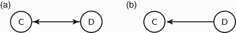
Figure 1.
Pictorial representation of an argumentation graph. Argument

As for notation, given an argumentation graph
We say that a sub-graph
Figure 2.
The graph (a) is a sub-graph of the graph in Figure 1, while the graph (b) is not one of its sub-graphs.
Once we have an argumentation graph, we can compute the set of arguments that are justified or rejected, that is, those arguments that shall survive or not to possible attacks. To do that, we need semantics. Many semantics exist and, for our purposes, we will consider Dung's grounded semantics (Dung, 1995) by labelling arguments as in Baroni et al. (2011), but slightly adapted to our purposes. Accordingly, we will distinguish
Definition 3.3
Definition 3.3Labellings
Let
A
A
A
Notice that the labelling functions are denoted with a lower case, reserving the upper case to denote random labellings in the probabilistic setting (as we will see in Section 4). We write
Definition 3.4
Definition 3.4Complete { in , out , un }
Let
A is labelled
A is labelled
An argumentation graph may have several complete
Definition 3.5
Definition 3.5Grounded { in , out , un }
Let
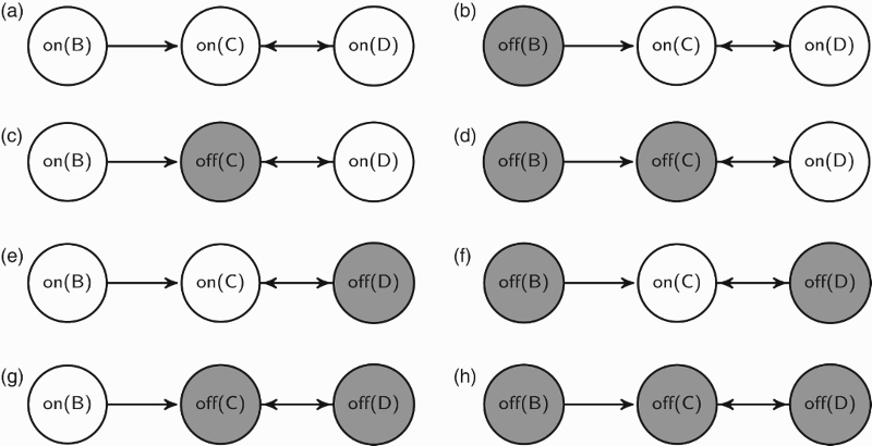
An algorithm for generating the grounded
This algorithm is sound because the resulting
We introduced
Definition 3.6
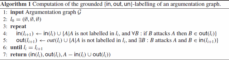
Definition 3.6Grounded { in , out , un , off }
Let
every argument in
every argument in
An argumentation graph has a unique grounded
Figure 3.
Grounded
As for notational matters, the sets of labellings of an argumentation graph
4.Probabilistic abstract argumentation framework
In this section, we introduce our probabilistic setting for the abstract argumentation framework as given in the previous section. Notice that there are many ways to define the probability space of a setting for probabilistic argumentation and the choice of a probability space shall be made in function of the envisaged applications. Our choice was conducted by the promotion of simplicity and to match our use of the graphical model of BMs for probabilistic argumentation towards the construction of neuro-argumentative systems.
So for our purposes, we define a sample space as the set of labellings of a hypothetical argumentation frame (or simply called a hypothetical frame) which is an argumentation graph. Now, when building a probabilistic setting, we have to make the distinction between between an impossible event (i.e. the event does not belong to the sample space), and an event with probability 0. Similarly, given a hypothetical argumentation frame
Definition 4.1
Definition 4.1Probabilistic argumentation frame
A probabilistic argumentation frame is a tuple
the sample space Ω is the set of labellings with respect to
the σ-algebra F is the power set of Ω,
the function P from
In the remainder, we may write
Example 4.2
Example 4.2continued
Assume a hypothetical argumentation frame as drawn in Figure 1. Considering the grounded
Figure 4.
Sample space as the set of
Remark that a probabilistic argumentation frame where the labelling is a
As we have defined our probabilistic space, we can consider random variables, that is, functions (traditionally defined by an upper case letter such as X) from the sample space Ω into another set of elements. So, we will associate to every argument A some random variables, called random labellings, to capture the random labelling of the argument.
Random labellings can take different forms. An option consists in considering binary random labellings, that we denote
(1)
We use boldface type to denote sets of random labellings, thus L denotes a set of random labellings
Given a set L of random labellings, we consider the standard definition of a factor as a function, denoted φ, from the possible set of assignments
(2)
(3)
If the scope of a factor contains two random labellings, then there is a direct probabilistic influence between these two random labellings. In this view, it is common to visualise dependences by relating a factorisation with a graphical structure, typically such as a Markov random field (MRF), also known as Markov network, where nodes represent random variables and arcs indicate dependences amongst these variables: in this case, a distribution
It is also common to visualise the factorisation under the graphical model of factor graphs, which is an alternative to Markov networks to explicit the factorisation. In this perspective, a factor graph for a set of random labellings
Example 4.3.
Consider an argumentation graph G with five arguments, say
(4)
Figure 5.
Tables corresponding to the factors
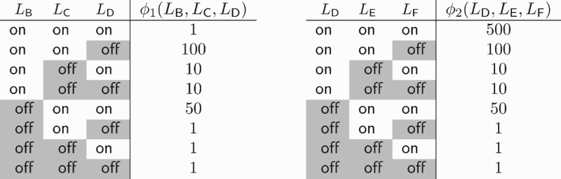
From the given factors, we can compute the joint probability of any
(5)
Graphical models provide a compact and graphical representation of dependences to deal with joint probability distributions. For example in MRFs, two sets of nodes A and B are conditionally independent given a third set C, if all paths between the nodes in A and B are separated by a node in C. In graphical models, arcs are thus meant to represent assumptions on conditional independence relationships amongst variables, and on the basis of these assumptions joint probability can break down into manageable products of conditional probabilities.
In abstract argumentation graphs, nodes represent arguments and arrows represent attacks. Though an attack necessarily indicates some sort of influence on the probability of justification of an argument, the structure of an argumentation graph is not meant to account for conditional independence relationships amongst arguments in the probabilistic sense.
For example, we could suppose that argument
Figure 6.
In this argumentation graph, arguments
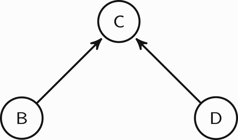
Clearly, the labelling of
Figure 7.
A MRF specifying explicit dependence amongst arguments
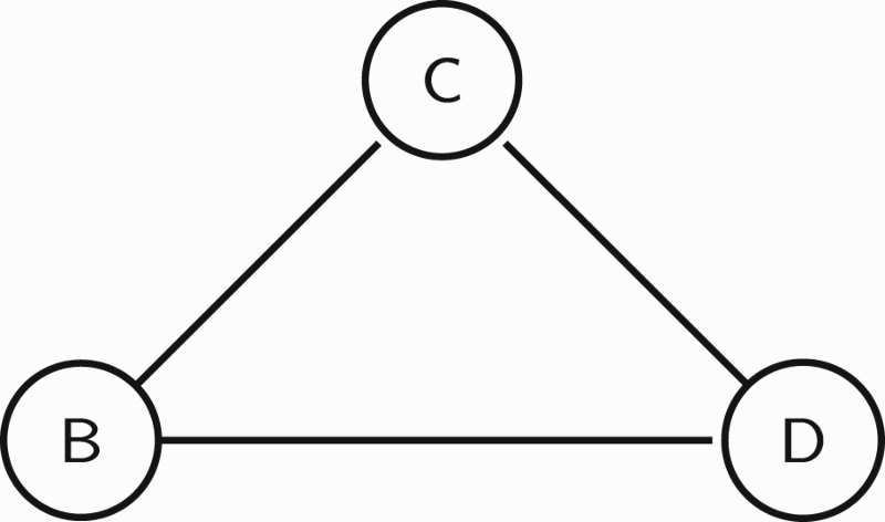
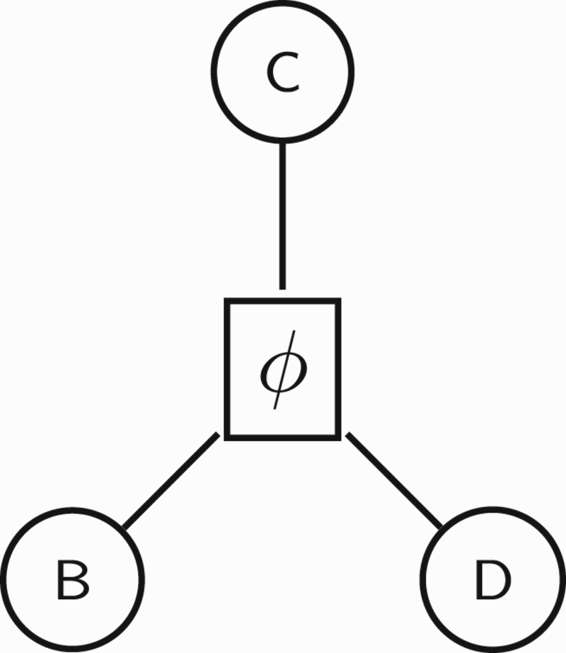
Figure 8.
A (trivial) factor graph specifying the joint probability
In this paper, we consider that graphs of probabilistic graphical models and argumentation graphs (and logical structures in general) are not meant to encode the same type of information (cf. Richardson and Domingos, 2006): graphs of probabilistic graphical models encode probabilistic dependence relations, while argumentation graphs encode logic constraints on the possible labellings amongst arguments. In this view, though graphs of probabilistic graphical models and argumentation carry distinct information, we see them as complementary, and an argumentation graph shall be associated with a probabilistic graphical model to specify probabilistic dependences.
If a Markov network is used as the probabilistic graphical model, then the dependencies can be given by a human operator, but they may also be discovered using some structure learning algorithms. An alternative is to introduce some hidden variables, represented by some binary hidden nodes in the Markov network, to account for unknown dependences. So assuming hidden variables, we may consider an assignment of binary random labellings l and the assignment of K binary hidden variables
(6)
Figure 9.
Graphical representation of pairwise graphical model with four hidden nodes of four hidden variables and three nodes of three categorical random labellings, such that there is no direct dependences between hidden variables or between random labellings.
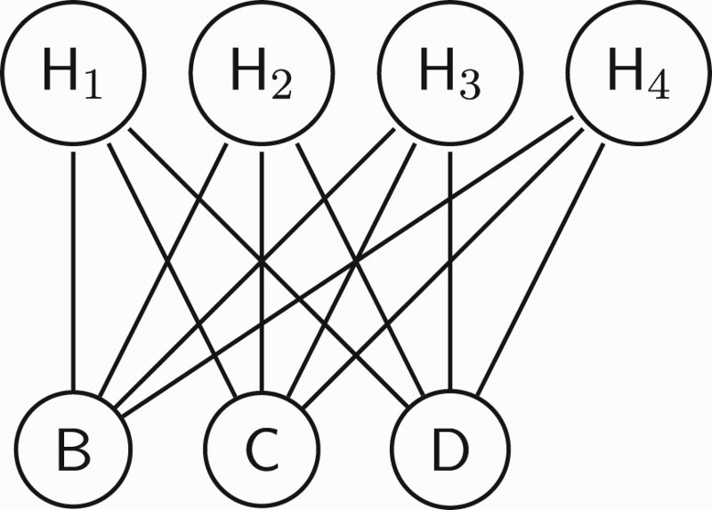
Figure 10.
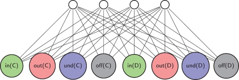
Graphical representation of a restricted BM with three hidden units and seven visible units. When the machine is interpreted as a neural network, each unit represents a neuron. When the machine is interpreted as a graphical model of a PoE, then each hidden unit represents an expert.
In such a bipartite graphical model, we may introduce a factor
(7)
As we will see, such a graphical model corresponds in fact to a particular graphical model of BMs called restricted Boltzmann machines (RBM). Using this model, we shall benefit for efficient learning algorithms to capture a compact model of a set of training examples, which can be accommodated to our probabilistic argumentation setting to discard illegal labelling (with respect to grounded
As the model of BMs is an energy-based model, we take the opportunity to present in the next section a counterpart energy-based model for our argumentation setting and its possible justification, and this will allow us to account for the settings investigated in Li et al. (2011), Fazzinga et al. (2013), and Dondio (2014) where arguments are probabilistically independent, as well as the setting of Riveret et al. (2012a,b) where the dependences amongst arguments are captured by a potential (which is a loose terminology for the energy function) meant to be learned by reinforcement learning.
5.Energy-based argumentation
Energy-based models in probabilistic settings associate an energy to any configuration defined by the variables of a system, and then associate a probability to each configuration on the basis of energies (see e.g. LeCun et al., 2006 for a tutorial).
Making an inference with an energy-based model consists in comparing the energies associated with various configurations of the variables, and choosing the one with the smallest energy. The energies of remarkable configurations can be given by a human operator, or they can be learned using machine learning techniques. In particular, any illegal configuration shall be set with an infinite energy, so that such configurations will occur with probability zero.
Energy-based models date back from the early work of statistical physics, notably the work of Boltzmann and Gibbs, and have since inspired more abstract probabilistic setting in particular so-called log-linear models in probabilistic graphical models. So energy-based models appear not only as a probabilistic setting with a strong theoretical basis, but have been shown to be useful in many practical applications. We are thus inspired by works using energy-based models, and we investigate here such energy-based models for argumentation. Sometimes, energy-based models are also called potential-based models, and we may favour the latter denomination to the former when we deal with argumentation, because it appears to us more natural to talk about the potential of arguments than the energy of arguments. However, we prefer here to align ourselves with the standard terminology of energy-based models. In the setting of argumentation, the energy can be interpreted as an opposite measure of the credit we put into the argumentative status of arguments, for example, the compatibility amongst the status taken by the arguments (a configuration). However, we shall not commit to any particular interpretation, and accordingly we shall use the word energy to designate it.
Using an energy-based account of probabilistic argumentation, we can use many concepts from statistical mechanics and information theory, such as entropy, and gain an intuitive understanding of the probabilistic setting. For example, the justification of such energy-based models can be found at the crossroad of information theory and statistical physics (see e.g. Jaynes, 1957), and we adapt it here for our argumentation setting.
Amongst possible configurations, it is a standard to accept the principle of insufficient reason (also called the principle of indifference): if there is no reason to prefer one configuration over alternatives, simply attribute the same probability to all of them. This principle dates back to Laplace when he was studying games of chance. A modern version of this principle is the principle of maximum entropy. In our setting, the entropy of a probability distribution of a set of labellings
(8)
However, the principle of insufficient reason has to be confronted to the principle of sufficient reason, which, in simple words, says that ‘nothing happens without a reason’. In our argumentative setting, the reason of the event of a labelling is fundamentally unknown, but such an event is nevertheless associated with an energy. The energy of a labelling
(9)
(10)
(11)
(12)
(13)
(14)
This distribution is also known as Gibbs or Boltzmann distribution and was historically first introduced in statistical mechanics to model gas. In counterpart systems studied in statistical physics, the constant β usually turns out to be inversely proportional to the temperature. In machine learning, this temperature is often used as a factor to ‘regularise’ the distribution over configurations or as parameter balancing the exploration and exploitation of alternative configurations, but for the sake of simplicity and because it is is not necessary for our purposes, we omit it here for our argumentative framework (by setting it to 1).
We discussed in the previous section the factorisation of a distribution in terms of dependences amongst random labellings, but we did not catered much for the form that factors can take. In this regard and in light of the above theoretical insights, it is standard to put the factorised distribution introduced in Equation (2) under the form of a log-linear model, so we write factors as exponentials:
(15)
Factors are meant to break down a full joint distribution into manageable pieces, but we are eventually interested to regroup all these pieces to get results for the full joint distribution. So, using the exponential form of factors of Equation (15) intoEquation (2), we obtain
(16)
If the arguments are assumed to be independent, we can associate one factor to every random labelling, and thus we obtain
(17)
(18)
(19)
(20)
(21)
(22)
Figuring out that a labelling l can be straightforwardly associated with an assignment l to every random labelling, we can write that the probability of a labelling is exponentially proportional to the overall energy of this labelling:
(23)
Using factorised probability distribution under the form of energy-based models, we have a direct connection with log-linear models of factor graphs and thus Markov networks as well as products of experts (see Section 6), so that well-established tools and techniques can be used for our present and future purposes.
In particular, when hidden variables are considered, we can write the factors in Equation (6) under the form of a log-linear model:
(24)
(25)
(26)
(27)
6.Boltzmann machines
The original BM (Ackley, Hinton, and Sejnowski, 1985) is a probabilistic undirected graphical model with binary stochastic units. The BM may be interpreted as a stochastic recurrent neural network and a generalisation of Hopfield networks (Hopfield, 1982) which feature deterministic rather than stochastic units. In contrast, however, to common neural networks, BMs are fully generative models, widely utilised for the purpose of feature extraction, dimensionality reduction and learning complex probability distributions.
The nodes of a BM are usually divided into observed (or visible) and latent (or hidden) units, where the former represent observations we wish to model and the latter capture the assumed underlying dependences among visible nodes. Postulating a BM of D visible and K hidden units, an assignment of binary values to the visible and hidden variables will be denoted as
(28)
(29)
(30)
As alluded to when introducing the use of such distribution in the previous section, and in order to reflect their physical meaning, the sum of energies
A BM is a special case of a MRF, where the energy function is chosen to be linear with respect to its inputs and more specifically of the following form:
(31)
Finally, an RBM is formed by dropping the connections between visible-to-visible and hidden-to-hidden units, by setting the corresponding transfer matrices L and J to zero. As a result, the joint model density can be formed as follows:
(32)
If the marginal probability of a configuration is sought, then it is common to introduce the free energy of a visible vector v, denoted
(33)
(34)
When training a machine, the primary objective is to estimate the optimal model weights
RBMs are usually trained by means of maximum likelihood estimation (MLE); although alternative approaches do exist in the literature, they usually introduce a significant computational burden. By employing MLE, we aim at estimating the optimal model parameter configuration
(35)
(36)
The first expectation is basically the entropy of
(37)
(38)
(39)
(40)
CD is based on a simple principle, according to which it is sufficient to approximate the expectations in Equation (40), using only one value of v and h. More specifically, we employ the following approximations:
(41)
(42)
(1) ‘Clamp’
(43)
(2) Draw
(44)
(3) Obtain
(45)
(46)
CD-k is applied by using the pair
(47)
(48)
(49)
(50)
(51)
The use of the logistic function in Equation (47) can be generalized to the case of a unit with K alternative states (such a unit is called a softmax unit), in this case the probability to draw the unit in the state j is as follows:
(52)
To generate samples from the learned model, Gibbs sampling is usually employed (Murphy, 2012), by iteratively sampling all random variables from their conditional probability densities. We also refer to that process as a ‘free run’. More specifically, we begin each free run from a random initial point
(53)
(54)
As the samples for learning and the samples in the generative mode are similarly drawn, BMs offer the possibility to learn a compact model of a distribution while drawing samples from the model. In this perspective, instead of reinitialising the Markov chain to an observed data point after each weight update, we may initialise the Markov Chain at the state in which it ended after k iterations, also referred as persistent CD (Tieleman, 2008).
Whatever the learning procedure, the number of hidden units used in an RBM has a strong influence on its ability to learn distributions. Roux and Bengio (2008) showed that when the number of hidden nodes of an RBM is increased, there are weight values for the new nodes that guarantee improvement in the KL divergence between the data distribution and the model distribution. In particular, they showed that any distribution over a set
7.Argumentative Boltzmann machines
To construct a BM that embodies abstract argumentation in our probabilistic setting, we reformulate argumentative labelling as a Gibbs sampling within the binary setting of BMs. Yet different machines can be built to perform the labelling of argumentation graphs in such setting. For this reason, we are in fact in front of different types of machines called argumentative Boltzmann machines in the sense that different machines can be proposed to label arguments. We are proposing two types here and we will focus on the second.
A first type of argumentative machine consists in a machine where the
To address the limitations of
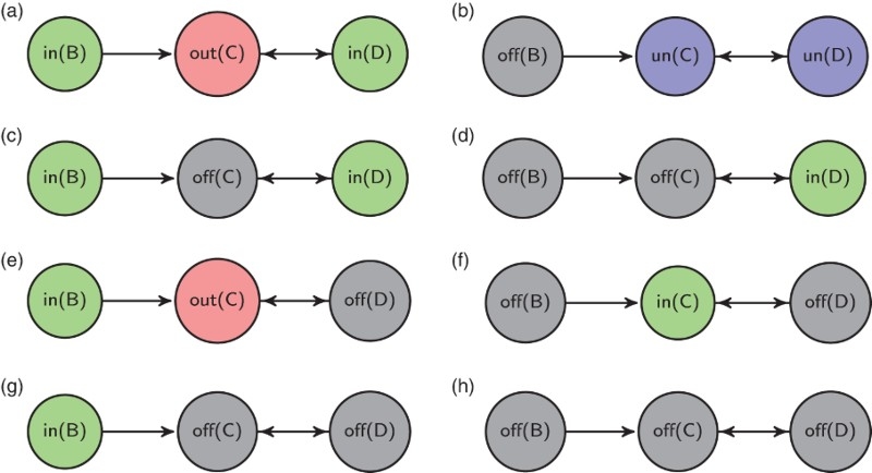
Figure 11.
A
An alternative
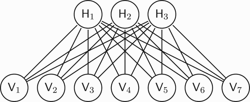
Figure 12.
An alternative

As for notation, the energy of activation of an argument A being labelled
An assignment v of the visible units corresponds to the assignment l of the binary random labellings associated with the set
(55)
(56)
(57)
Focusing on grounded
To ensure the production of grounded
For the sake of the clarity of the presentation, we adopt the following notation. An argument A is labelled
A is not labelled in
A is drawn
We denote
An argument A is labelled
A is not labelled in
A is drawn
We denote
An argument A is labelled
A is not labelled in
A was not labelled
We denote
Finally, an argument A is labelled
A is not labelled in
A is drawn
We denote
With this notation, we can now present a simple version of the grounded
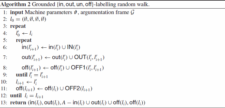
The labelling random walk consists of an outer loop and an inner loop. The inner loop draws the labelling
When learning, the machine will be shown a set of training examples where an example is a set of labelled arguments. To clamp the visible nodes of a machine with a set of labelled arguments, a visible node will be set at 1 if its labelling matches the example, otherwise it is set at 0. If a training example does not match any grounded
When labelling arguments with the labelling random walk, if the weight matrix L is not set to 0 (e.g. in the case of a general BM), then the order in which the arguments are labelled matters. If the matrix L is set to 0, as in the case of an RBM, then the order of labelling does not matter. Thus, a grounded
As an RBM can be interpreted as a PoE, we may interpret the labelling walk as the walk of a judge when given a coherent judgement concerning the status of arguments. At each step, the judge asks the advice of every expert (i.e. to every hidden node) to label the arguments, and this labelling occurs with respect to the constraints of a grounded labelling of the hypothetical argumentation frame. At the termination of the walk, the judge returns a labelling status to all the arguments of the frame.
Now, the hidden layer of BMs is often meant to extract features from input samples. The weights of each hidden unit represent those features, and define the probability that those features are present in a sample. For example, in face recognition, hidden units shall learn features such as edges at given orientations and positions, and these features shall be combined to detect facial features such as the nose, mouth or eyes. In argumentation, some sorts of labelling patterns may be captured by hidden nodes, and experiments in Section 8 will shed some lights on these considerations.
Example 7.1.
Let us illustrate the grounded
suppose
suppose
suppose
The resulting labelling is thus
suppose
suppose
suppose
So in this last walk, the labelling
For any possible input, the grounded
Theorem 7.2
Theorem 7.2Termination
The grounded
Proof.
To prove the termination, we consider the sequence of pairs
We say that a labelling algorithm is sound with respect to a type of labelling if, and only if, it returns a labelling of the argumentation frame as defined with respect to this type of labelling. When the grounded
Theorem 7.3
Theorem 7.3Soundness
The grounded
Proof.
To prove the soundness, we consider any terminated sequence
Moreover, we say that a labelling algorithm is complete with respect to a type of labelling if, and only if, it can return any labelling of the argumentation frame as defined with respect to this type of labelling. The grounded
Theorem 7.4
Theorem 7.4Completeness
The grounded
Proof.
To prove the completeness, we demonstrate that for any grounded
As mentioned earlier, once a machine is trained, the free energy of any illegal labelling shall be very high compared to legal labellings, in a manner such that the probability of any illegal labelling will be close to 0. So, a standard Gibbs sampling may sample illegal labellings with probability close to 0. Since the grounded
Concerning time complexity, the walk is a slight adaptation of Algorithm 1 for a probabilistic setting, meant to keep its polynomial complexity.
Theorem 7.5
Theorem 7.5Time complexity
Time complexity of the grounded
Proof.
At each iteration of the inner loop, one argument at least is labelled, otherwise the algorithm terminates. Therefore, when the input argumentation frame has N arguments, then there are N iterations at worse. For each iteration, the status of N argument has to be checked with respect to the status of N arguments in the worst case. The time complexity of this inner loop is thus polynomial. When the inner loop terminates, one iteration of the outer loop completes by checking the status of remaining unlabelled arguments, and the outer loop iterates N times at worse. Therefore, the time complexity of the grounded
Concerning space complexity, a major benefit of the proposed approach is to tackle the exponential space complexity of the sample space of a probabilistic argumentation frame (see Definition 4.1) by a compact machine whose the space complexity is reduced to weight matrices.
Theorem 7.6
Theorem 7.6Space complexity
Space complexity of the grounded
Proof.
A BM can be described by two binary random vectors corresponding to nodes vectors v and h, and matrices L, J and W (corresponding to the strength of the edges between hidden and visible nodes, see Figure 11), an hypothetical argumentation graph and machine parameters. The two binary vectors, the hypothetical argumentation graph and machine parameters require minimal space, thus the memory requirements are dominated by the real-valued edge matrices L, J and W. We need a weight to describe each pairwise interaction amongst hidden and visible nodes, thus it holds that the dimensions of the matrices are
In case of an RBM, we have
The labelling random walk is designed to ensure the production of grounded
8.Experiments
The experiments regard the use and effects of the grounded
To get experimental insights into the use of the grounded
The statistical distance between the empirical distribution P of the labellings drawn from a training dataset (approximating the source distribution) and the distribution
(58)
The experiments concerned (i) a tiny hypothetical argumentation frame so that the source distribution, the distribution of reconstructed labellings (at the end of a training phase) and the distribution of generated labellings (at the end of a generative phase) could be extensively compared and that the weights could be examined (ii) a small hypothetical argumentation frame to test RBMs with different argumentative mixing rates and entropies of the training distributions (iii) larger frames to reconnoiter the limits of the tested machines. In all cases, the datasets were artificially generated (without any noise), so that this evaluation was not dependent of any particular domain. To build these datasets, each grounded
8.1.First experiment
The first experiment regards the training of a grounded
Figure 13.
The hypothetical argumentation frame used for the first experiment.

The training consisted of 1000 passes over small batches, each containing 100 grounded
We present in Table 1 a comparison of the source distribution, the distribution of reconstructed labellings (taken from the 500th weight update to the last update of the training) and the distribution of generated labellings (at the end of a generative phase of the same duration than the CD-4 training phase). Numbers are rounded off.
Table 1.
Comparing the empirical probability distribution of a source training set of labellings (
| 0.158 | 0.157 | 0.161 |
| 0.13 | 0.13 | 0.127 |
| 0.129 | 0.127 | 0.125 |
| 0.106 | 0.103 | 0.104 |
| 0.071 | 0.071 | 0.068 |
| 0.071 | 0.07 | 0.069 |
| 0.048 | 0.046 | 0.043 |
| 0.047 | 0.046 | 0.046 |
| 0.047 | 0.045 | 0.047 |
| 0.039 | 0.039 | 0.041 |
| 0.039 | 0.037 | 0.038 |
| 0.021 | 0.021 | 0.023 |
| 0.012 | 0.013 | 0.012 |
| 0.012 | 0.012 | 0.012 |
| 0.01 | 0.01 | 0.01 |
| 0.008 | 0.007 | 0.006 |
| 0.008 | 0.008 | 0.007 |
| 0.005 | 0.007 | 0.006 |
| 0.005 | 0.006 | 0.007 |
| 0.005 | 0.005 | 0.005 |
| 0.005 | 0.005 | 0.003 |
| 0.004 | 0.006 | 0.01 |
| 0.004 | 0.006 | 0.007 |
| 0.004 | 0.005 | 0.004 |
| 0.002 | 0.005 | 0.007 |
| 0.002 | 0.002 | 0.005 |
| 0.002 | 0.004 | 0.003 |
| 0.002 | 0.002 | 0.002 |
| 0.001 | 0.001 | 0.002 |
| 0.001 | 0.002 | 0.001 |
| 0.001 | 0.002 | 0.001 |
| 0 | 0 | 0 |
Notes: The resulting KL divergence for the training period is 0.005 and the TV distance is 0.017. The resulting KL divergence for the generative period is 0.01 and the TV distance is0.029.
As the table shows, the machine reconstructed the labellings in the training phase and generated the labellings in the generated phase according to a probability distribution closed to the source distribution.
Since the graphical model of a RBM can be interpreted as a PoE, where each hidden node is an expert, we can wonder whether this interpretation shall reflect in the weights learned during the training. For example, we can wonder whether an expert shall clearly favour a particular
To inspect whether we can retrieve some labelling patterns from the weights given by the experts after training, we display the weights learned by two experts in Figure 14. As the weights show, the first expert did not appear to frankly back any particular labelling. The second expert seemed to favour labellings where the argument
Figure 14.
Two trained experts, (a) and (b). Each table shows the weights given by an expert to the alternative labellings of arguments.
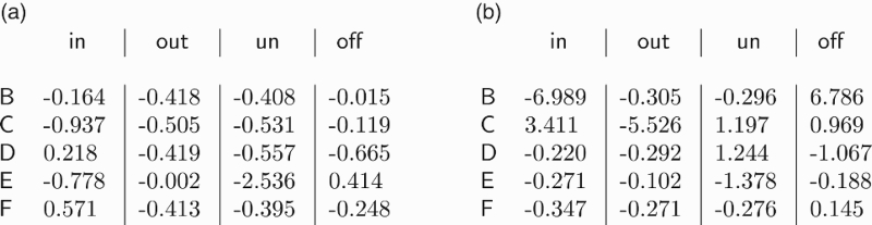
We conclude that a trained expert will not necessarily favour a particular labelling in any sharp manner, though some parts of labellings may be identified. As an analogy, we have a judge in front of a brouhaha of experts, and astonishingly enough, this judge will manage to label arguments by making the product of the expertises.
8.2.Second set of experiments
The second experiment regarded the performance of machines with respect to different entropies of the source distribution and for the hypothetical argumentation frame shown in Figure 15. With this frame,
Figure 15.
A hypothetical argumentation frame used for our second experiment.

The training consisted of 4000 passes over mini-batches, each containing 200 grounded
We evaluated the machines by keeping track of the TV distance averaged over 100 different datasets, each dataset having a different entropy. Figure 16 shows, for different argumentative mixing rates, the tracked distances between (i) the source distribution and the distribution of reconstructed labellings (taken from the 2000th weight update to the last update of the training) and (ii) the source distribution and the distribution of generated labellings (at the end of a generative phase of the same duration than the CD-4 training phase from the 2000th weight update to the last update of the training). The KL divergence was not tracked because it may not be defined when some labellings are produced with a probability zero, especially when the learning is initiated. We show the runs for the cases where
the mixing rate is 1 for the learning and the generative mode. This setting corresponds to a conventional RBM.
the mixing rate is 0.5 for the learning and the generative mode. In this setting, visible nodes are sampled with the grounded
the mixing rate is 0 for the learning and the generative mode. In this setting, visible nodes are always sampled with the grounded
the mixing rate is 1 for a first learning phase and 0 in a second learning phase, and then 0 for the generative mode.
Figure 16.
Progression of the TV distance for RBMs for different argumentative mixing rates. Results are averaged over 100 runs, each run learning a different dataset.
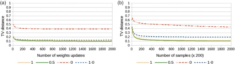
We observe that a conventional machine exhibits a similar convergence than a balanced mixed machine. In comparison, a pure argumentative machine does not perform well. We conjuncture that the reason holds in that pure argumentative machines (
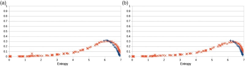
We give in Figure 17 the resulting statistical distances with respect to different entropies. The figures reveal a dispersion of the distances for distributions towards high entropies (up to a point where the statistical distances shall decrease for extreme entropies). The results also show that a balanced argumentative machine shall perform slightly better than a conventional machine. Of course such results hold for the experimental setting: one can better deal with high entropies by augmenting the number of hidden units (as we will see soon) or by simply increasing the training time for example. Moreover, we can expect that, in practice, argumentative routines shall bring distributions of labellings towards regions of low entropy.
Besides, the labelling walk is independent of the learning algorithm of a conventional BM, thus we should be able to train a machine as a conventional machine, use the labelling walk (in order to sample grounded
Figure 17.
Statistical distances (KL divergence and TV distance) resulting after a training phase and a generative phase versus the entropy of the training probability distributions. (a) Learning mode with a mixing rate
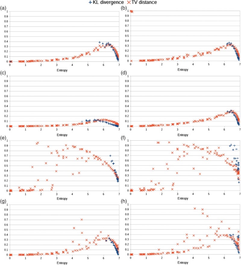
Figure 18.
Statistical distances (KL divergence and TV distance) after a training phase and a generative phase versus the entropy of the training probability distributions. By definition of the experimental setting, the distances for the training mode are the distances of a conventional machine. (a) Learning mode with a mixing rate
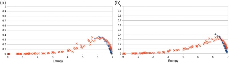
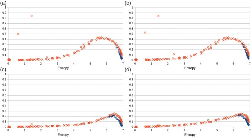
So far, we used
Figure 19.
Statistical distances (KL divergence and TV distance) resulting after a training phase and a generative phase versus the entropy of the training probability distributions, for a
When overviewing BMs in Section 6, we mentioned that the number of hidden nodes used in an RBM influences its ability to learn distributions: as shown by Roux and Bengio (2008), when the number of hidden nodes of an RBM is increased, there are weight values for the new nodes that guarantee improvement in the KL divergence between the data distribution and the model distribution. This theoretical influence of the number of the hidden nodes on learning can be seen in Figure 20, where we can observed that a machine with 60 hidden nodes perform better than a machine with 15 nodes. These results also suggest that few hidden nodes shall be sufficient when modelling distributions with low entropies. When the entropy is 0, then the biases shall suffice to capture the considered labelling (which has a probability 1).
Figure 20.
Statistical distances (KL divergence and TV distance) resulting after a training phase and a generative phase versus the entropy of the training probability distributions, for a
In light of these experiments, the labelling random walk appears thus as a mean to sample valid labellings on demand, without degraded performance with respect to a conventional RBM, and even with possible improvements. We show that a conventional learning algorithm shall be used for training, and a labelling walk can be used to generate grounded labellings. Thus, one can take advantage of massive parallel computation offered by the graphical model of RBMs to speed up the training. Furthermore, since the labelling walk is well separated from the learning procedure, we can take advantages of variants of such procedures and future improvements. By increasing the number of sampled grounded
8.3.Third set of experiments
We completed our experimental insights by extending the hypothetical argumentation frame with up to 20 arguments. We considered 10 frames, from 10 arguments to 20 arguments. In order to provide a compact and visual representation, we present each frame under the form of a submatrix of the adjacency matrix
Figure 21.
Adjacency matrix encoding argumentation graphs.

We kept the training setting of the second experiment for machines with an argumentative mixing rate 0.5, with the exception of the duration of the training and generative phases: in this experiment the training consisted of 6000 passes over mini-batches. We evaluated the machines by keeping track of the TV distances for four runs for the different frames and for two entropies of datasets, 3.466 and5.198.
The resulting TV distances are given in Figure 22, for the two entropies 3.466 and 5.198, between (i) the source distribution and the distribution of reconstructed labellings (taken from the 2000th weight update to the last update of the training) and (ii) the source distribution and the distribution of generated labellings (at the end of a generative phase of the same duration than the CD-4 training phase from the 2000th weight update to the last update of the training).
Figure 22.
TV distances resulting after a learning phase and a generative phase (with a mixing rate
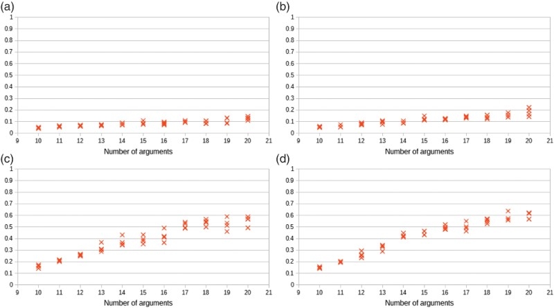
We observe that learning degrades when the number of arguments augments and when the entropy increases. Results shall improve with a longer training, or by considering more advanced learning settings such as persistent contrastive learning (Tieleman, 2008), stacked RBMs (i.e. deep BMs, see Salakhutdinov and Hinton, 2009) or some assumptions concerning the probabilistic dependences amongst arguments (as in the spirit of factor graphs). Such settings are left for future investigations.
9.Conclusion
We investigated an integration of abstract argumentation and probability theory with undirected graphical models and in particular with the graphical model of BMs. This combination allows us to relax assumptions on probabilistic independences amongst arguments, along a possible closed-form representation of a probabilistic distribution. We focused on generative learning, and we proposed a random labelling walk to generate grounded labellings ‘on demand’, while possibly keeping conventional training procedures. Thus, we can take advantage of massive parallel computation offered by the graphical model of RBMs to speed up the training. Since the labelling walk is well separated from the learning procedure, we can take advantages of variants of such learning procedures and future improvements. It also offers the possibility to learn on the fly a probability distribution of labelled arguments while producing labellings sampled according to the learned distribution.
Since the model of BMs is commonly interpreted as a model of neural networks, we are thus moving towards the construction of neuro-argumentative systems based on a principled account of probabilistic argumentation. Moreover, as the graphical model of RBMs can also be interpreted as a PoE, our contribution can also interpreted as a probabilistic model of an assembly of experts judging the status of arguments.
Future developments can be multiple, they range from instantiation of the abstract argumentation into specific frameworks (e.g. rule-based argumentation, see Riveret et al. (2015) for a setting which accounts for sub-arguments) to further benchmarking of variants of BMs such as deep machines for learning and inference in probabilistic argumentation. Different semantics may be addressed, and the modifications of hypothetical argumentation frames may be considered to account for unforeseen argumentative dependences. Towards structure learning, weights of argumentative machines shall be interpreted in order to extract the structure of hypothetical argumentation graphs. Finally, the utility of the approach has to be investigated by learning from labelled data in real applications instead of artificial distributions.
Disclosure statement
No potential conflict of interest was reported by the authors.
References
1 | Ackley D. H., Hinton G. E., & Sejnowski T. J. ((1985) ). A learning algorithm for Boltzmann machines*. Cognitive Science, 9: , 147–169. doi: 10.1207/s15516709cog0901_7 |
2 | Baroni P., Caminada M., & Giacomin M. ((2011) ). An introduction to argumentation semantics. Knowledge Engineering Review, 26: , 365–410. doi: 10.1017/S0269888911000166 |
3 | Baroni P., Giacomin M., & Vicig P. ((2014) ). On rationality conditions for epistemic probabilities in abstract argumentation. Proceedings of computational models of argument: Vol. 266. Frontiers in artificial intelligence and applications (pp. 121–132). IOS Press. |
4 | Bondarenko A., Dung P. M., Kowalski R. A., & Toni F. ((1997) ). An abstract, argumentation-theoretic approach to default reasoning. Artificial Intelligence, 93: , 63–101. doi: 10.1016/S0004-3702(97)00015-5 |
5 | Cayrol C., & Lagasquie-Schiex M.-C. ((2013) ). Bipolarity in argumentation graphs: towards a better understanding. International Journal of Approximate Reasoning, 54: , 876–899. doi: 10.1016/j.ijar.2013.03.001 |
6 | d'Avila Garcez A. S., Gabbay D. M., & Lamb L. C. ((2005) ). Value-based argumentation frameworks as neural-symbolic learning systems. Journal of Logic and Computation, 15: , 1041–1058. doi: 10.1093/logcom/exi057 |
7 | d'Avila Garcez A. S., Gabbay D. M., & Lamb L. C. ((2014) ). A neural cognitive model of argumentation with application to legal inference and decision making. Journal of Applied Logic, 12: , 109–127. doi: 10.1016/j.jal.2013.08.004 |
8 | d'Avila Garcez A. S., Lamb L., & Gabbay D. ((2008) ). Neural-symbolic cognitive reasoning (1st ed.). Springer. |
9 | De Finetti B. ((1974) ). Theory of probability: a critical introductory treatment. Wiley. |
10 | Dondio P. ((2014) ). Toward a computational analysis of probabilistic argumentation frameworks. Cybernetics and Systems, 45: , 254–278. doi: 10.1080/01969722.2014.894854 |
11 | Dung P. M. ((1995) ). On the acceptability of arguments and its fundamental role in nonmonotonic reasoning, logic programming and n-person games. Artificial Intelligence, 77: , 321–357. doi: 10.1016/0004-3702(94)00041-X |
12 | Dung P. M., & Thang P. M. ((2010) ). Towards (Probabilistic) argumentation for jury-based dispute resolution. Proceedings of the 2010 conference on computational models of argument, COMMA'10 (pp. 171–182). IOS Press. |
13 | Fazzinga B., Flesca S., & Parisi F. ((2013) ). On the complexity of probabilistic abstract argumentation. IJCAI, IJCAI/AAAI. |
14 | Fruhwirth T. ((2009) ). Constraint Handling Rules (1st ed.). Cambridge University Press. |
15 | Getoor L., Friedman N., Koller D., Pfeffer A., & Taskar B. ((2007) ). Probabilistic relational models. An introduction to statistical relational learning. MIT Press. |
16 | Getoor L., & Taskar B. ((2007) ). Introduction to statistical relational learning (Adaptive computation and machine learning). The MIT Press. |
17 | Governatori G., Maher M. J., Billington D., & Antoniou G. ((2004) ). Argumentation Semantics for Defeasible Logic. Journal of Logic and Computation, 14: , 675–702. doi: 10.1093/logcom/14.5.675 |
18 | Governatori G., Rotolo A., & Sartor G. ((2005) ). Temporalised normative positions in defeasible logic. In Proceedings of the 10th International Conference on Artificial Intelligence and Law (pp. 25–34). ACM. |
19 | Hinton G. E. ((2002) a). Training products of experts by minimizing contrastive divergence. Neural Computation, 14: , 1771–1800. doi: 10.1162/089976602760128018 |
20 | Hinton G. E. ((2002) b). Training products of experts by minimizing contrastive divergence. Neural Computation, 14: , 1771–1800. doi: 10.1162/089976602760128018 |
21 | Hinton, G. ((2012) ), “A Practical Guide to Training Restricted Boltzmann Machines,” Vol. 7700: , Springer Berlin Heidelberg, pp. 599–619. |
22 | Hinton A., Kwiatkowska M., Norman G., & Parker D. ((2006) ). PRISM: A tool for automatic verification of probabilistic systems. Proceedings of the 12th international conference on tools and algorithms for the construction and analysis of systems, TACAS'06 (pp. 441–444). Springer. |
23 | Hopfield J. J. ((1982) ). Neural networks and physical systems with emergent collective computational abilities. Proceedings of the National Academy of Sciences, 79: , 2554–2558. doi: 10.1073/pnas.79.8.2554 |
24 | Hunter A. ((2013) ). A probabilistic approach to modelling uncertain logical arguments. International Journal of Approximating Reasoning, 54: , 47–81. doi: 10.1016/j.ijar.2012.08.003 |
25 | Hunter A., & Thimm M. ((2014) ). Probabilistic argumentation with epistemic extensions and incomplete information. CoRR, abs/1405.3376. |
26 | Jaynes E. T. ((1957) ). Information theory and statistical mechanics. Physical Review, 106: , 620–630. doi: 10.1103/PhysRev.106.620 |
27 | Koller D., & Friedman N. ((2009) ). Probabilistic graphical models: principles and techniques – adaptive computation and machine learning. The MIT Press. |
28 | LeCun Y., Chopra S., Hadsell R., Ranzato M., & Huang F. ((2006) ). A tutorial on energy-based learning. In G. Bakir, T. Hofman, B. Schölkopf, A. Smola & B. Taskar (Eds.), Predicting structured data. MIT Press. |
29 | Li S. Z. ((1995) ). Markov random field modeling in computer vision. Springer. |
30 | Li H. ((2015) ). Probabilistic argumentation. University of Aberdeen. |
31 | Li H., Oren N., & Norman T. J. ((2011) ). Probabilistic argumentation frameworks. Revised selected papers of first international workshop theory and applications of formal argumentation, TAFA'11. Lecture Notes in Computer Science (pp. 1–16). Springer. |
32 | Modgil S., & Caminada M. ((2009) ). Proof theories and algorithms for abstract argumentation frameworks. Argumentation in artificial intelligence. Springer, pp. 105–129. |
33 | Mozina M., Zabkar J., & Bratko I. ((2007) ). Argument based machine learning. Artificial Intelligence, 171: , 922–937. doi: 10.1016/j.artint.2007.04.007 |
34 | Murphy K. P. ((2012) ). Machine learning: a probabilistic perspective. MIT press. |
35 | Nute D. ((2001) ). Defeasible logic. Handbook of logic in artificial intelligence and logic programming. Oxford University Press, pp. 353–395. |
36 | Paolucci M., Kossmann D., Conte R., Lukowicz P., Argyrakis P., Blandford A., … Helbing D. ((2013) ). Towards a living earth simulator. CoRR, abs/1304.1903. |
37 | Prakken H., & Sartor G. ((1997) ). Argument-based extended logic programming with defeasible priorities. Journal of Applied Non-Classical Logics, 7: . doi: 10.1080/11663081.1997.10510900 |
38 | Rahwan I. ((2008) ). Mass argumentation and the semantic web. Web Semantics: Science, Services and Agents on the World Wide Web, 6: , 29–37. doi: 10.1016/j.websem.2007.11.007 |
39 | Richardson M., & Domingos P. ((2006) ). Markov logic networks. Machine Learning, 62: , 107–136. doi: 10.1007/s10994-006-5833-1 |
40 | Riveret R., Pitt J. V., Korkinof D., & Draief M. ((2015) ). Neuro-symbolic agents: Boltzmann machines and probabilistic abstract argumentation with sub-arguments. Proceedings of the 2015 international conference on autonomous agents and multiagent systems, AAMAS (pp. 1481–1489). |
41 | Riveret R., Prakken H., Rotolo A., & Sartor G. ((2008) ). Heuristics in argumentation: a game theory investigation. Proceedings of computational models of argument, COMMA'08, Vol. 172 of Frontiers in artificial intelligence and applications (pp. 324–335). IOS Press. |
42 | Riveret R., Rotolo A., & Sartor G. ((2012) a). Norms and learning in probabilistic logic-based agents. Proceedings of the 11th international conference in deontic logic in computer science, DEON'12: Vol. 7393. Lecture notes in computer science (pp. 123–138). Springer. |
43 | Riveret R., Rotolo A., & Sartor G. ((2012) b). Probabilistic rule-based argumentation for norm-governed learning agents. Artificial Intelligence and Law, 20: , 383–420. doi: 10.1007/s10506-012-9134-7 |
44 | Riveret R., Rotolo A., Sartor G., Prakken H., & Roth B. ((2007) ). Success chances in argument games: a probabilistic approach to legal disputes. Proceeding of the 20th conference on legal knowledge and information systems, JURIX'07 (pp. 99–108). IOS Press. |
45 | Roth B., Riveret R., Rotolo A., & Governatori G. ((2007) ). Strategic argumentation: a game theoretical investigation. Proceedings of the 11th international conference on artificial intelligence and law, ICAIL'07 (pp. 81–90). ACM. |
46 | Roux N. L., & Bengio Y. ((2008) ). Representational power of restricted Boltzmann machines and deep belief networks. Neural Computation, 20: , 1631–1649. doi: 10.1162/neco.2008.04-07-510 |
47 | Salakhutdinov R., & Hinton G. E. ((2009) ). Deep Boltzmann machines. In Proceedings of the Twelfth International Conference on Artificial Intelligence and Statistics, AISTATS: Vol. 5. JMLR Proceedings (pp. 448–455). |
48 | Sartor G. ((2005) ). Legal reasoning: a cognitive approach to the law. Springer. |
49 | Sato T. ((2008) ). A glimpse of symbolic-statistical modeling by PRISM. Journal of Intelligent Information Systems, 31: , 161–176. doi: 10.1007/s10844-008-0062-7 |
50 | Schneider J., Groza T., & Passant A. ((2013) ). A Review of Argumentation for the Social Semantic Web. Semantic Web, 4: , 159–218. |
51 | Sneyers J., Meert W., Vennekens J., Kameya Y., & Sato T. ((2010) ). CHR(PRISM)-based probabilistic logic learning. CoRR, abs/1007.3858. |
52 | Sneyers J., Schreye D. D., & Fruhwirth T. ((2013) ). Probabilistic legal reasoning in CHRiSM. Theory and Practice of Logic Programming, 13: , 769–781. doi: 10.1017/S1471068413000483 |
53 | Thimm M. ((2012) ). A probabilistic semantics for abstract argumentation. Proceedings of the 20th European conference on artificial intelligence, ECAI'12, Vol. 242 of Frontiers in artificial intelligence and applications (pp. 750–755). IOS Press. |
54 | Tieleman T. ((2008) ). Training restricted Boltzmann machines using approximations to the likelihood gradient. Proceedings of the 25th international conference on machine learning (pp. 1064–1071). ACM. |
55 | Torroni P., Gavanelli M., & Chesani F. ((2007) ). Argumentation in the semantic web. IEEE Intelligent Systems, 22: , 66–74. doi: 10.1109/MIS.2007.100 |
56 | Torroni P., Gavanelli M., & Chesani F. ((2009) ). Arguing on the semantic grid. Argumentation in artificial intelligence. Springer, pp. 423–441 (chap. 21). |


