
AAD and least-square Monte Carlo: Fast Bermudan-style options and XVA Greeks
Abstract
We show how Adjoint Algorithmic Differentiation (AAD) can be used to calculate price sensitivities in regression-based Monte Carlo methods reliably and orders of magnitude faster than with standard finite-difference approaches. We present the AAD version of the celebrated least-square algorithms of Tsitsiklis and Van Roy (2001) and Longstaff and Schwartz (2001). By discussing in detail examples of practical relevance, we demonstrate how accounting for the contributions associated with the regression functions is crucial to obtain accurate estimates of the Greeks, especially in XVA applications.
1Introduction
The efficient calculation of the risk factor sensitivities of financial derivatives, also known as the “Greeks”, is an essential component of modern risk management practices. Indeed, the aftermath of the recent financial crisis has seen remarkable changes in the market practice whereby financial institutions need to quantify (and risk-manage) counterparty, funding and capital exposures, collectively known as XVA, in large portfolios, see e.g., Crépey et al. (2014).
The traditional approach for the calculation of the Greeks is the so-called bump and reval or bumping technique. This comes with a significant computational cost as it generally requires repeating the calculation of the P&L of a portfolio under hundreds of market scenarios in order to form finite-difference estimators. As a result, in many cases, even after deploying vast amounts of computer power, these calculations cannot be completed in a practical amount of time.
Conversely, Adjoint Algorithmic Differentiation (AAD), a numerical technique recently introduced to financial engineering (see e.g., Capriotti (2011); Capriotti et al. (2011); Capriotti and Giles (2012, 2010); Henrard (2014)), has proven to be effective for speeding up the calculation of risk factor sensitivities, both for Monte Carlo (MC) and deterministic numerical methods, see Capriotti and Lee (2014); Savickas et al. (2014); Capriotti et al. (2015); Xu et al. (2016); Geeraert et al. (2017).
The main ideas underlying AAD can be illustrated by considering a computer implemented function of the form
(1)
(2)
Here, the real-valued vectors U and V represent intermediate variables utilised in the calculation. Each step may be a distinct high-level function or even a specific instruction.
AAD, sometimes also simply known as adjoint mode of Algorithmic Differentiation (AD), results from “propagating” the derivatives of the final output with respect to all the intermediate variables – the so called adjoints – until the derivatives with respect to the independent variables are formed. Using the standard AD notation, the adjoint of any intermediate variable Vk is defined by
(3)
Starting from the adjoint of the outputs
(4)
(5)
One particularly important theoretical result is that given a computer program performing some high-level function (1), the execution time of its adjoint counterpart
(6)
(7)
In this paper we present the application of AAD to regression-based MC approaches (also known as least-square MC) such as those that are widely utilised for Bermudan-style options, see Carriere (1996); Tsitsiklis and Van Roy (2001); Longstaff and Schwartz (2001), or for XVA applications, see Cesari et al. (2009) and Joshi and Kwon (2016). We develop the AAD implementation of the well-known least-square algorithm for the computation of conditional expectations, and we investigate numerically the impact on the Greeks arising from the sensitivities of the regression functions, a component that is generally ignored for Bermudan-style options by invoking arguments of quasi-optimality of the exercise boundary.
The paper is organised as it follows: In the next section, the regression-based MC algorithm for both Bermudan-style options and XVA is presented. In Section 3 we discusses the AAD algorithms for the regression-based MC method. We give two numerical examples, the best of two stocks Bermudan-style call and its corresponding XVA in Section 4. Here we show how smoothening out discontinuities associated with suboptimal exercise boundaries improves the accuracy of the Greeks of Bermudan-style options, and why the contribution to the sensitivities arising from the regression boundaries is essential for an accurate computation of XVA sensitivities. The efficiency and accuracy of AAD is also compared with bump and reval approaches in the same section.
2Valuation of Bermudan-style options and XVA by regression-based Monte Carlo
2.1Bermudan-style options
While European-style options can be exercised only at final maturity, Bermudan-style options can be exercised on multiple dates up to trade expiry.
We denote by T1, …, TM the exercise dates of the option and define
A rational investor will exercise the option that he holds in such a way as to maximise its economic value. As a result, the value of a Bermudan-style option is the supremum of the option value over all possible exercise policies. With the notation introduced above, the value of a Bermudan-style option at time t can thus be expressed by
(8)
A useful concept is the hold value of the Bermudan-style option: We denote by H (t) the value of the Bermudan-style option when the exercise dates are restricted to
(9)
The option holder, following an optimal exercise policy, will exercise his option if the exercise value is larger than the hold value, i.e.,
(10)
This, when combined with Equation (9), leads to the so-called dynamic programming formulation:
(11)
The dynamic programming formulation above implies that the stopping time, defining the optional exercise date as seen at time t, is given by
(12)
The optimal exercise strategy defined by Equation (12) requires the computation of the hold value H (t), m = η (t) + 1, …, M - 1. In a setting in which the underlying risk factor process {X (t) } 0≤t≤T is a generic k-dimensional Markov process, the hold value H (t) is a function of the state vector at time t. That is,
(13)
When the dimension of the Markov process k is small enough, the conditional expectation value in Equation (13) can be computed in a straightforward way by discretising the risk-factor process and performing standard backward induction on a tree or a grid, or by discretising an associated Partial Differential Equation (PDE). Here we refer to, e.g., Wilmott et al. (1995). However, the complexity of grid-based calculations is exponential in the dimension of the Markov process and numerical implementations become infeasible when k ≥ 4.
As we will review in Section 2.3, regression-based MC techniques provide an effective way of computing conditional expectation values of the form (13).
2.2XVA
We next consider the computation of the Credit Valuation Adjustment (CVA) and the Debt Valuation Adjustment (DVA) as the main measures of a dealer’s counterparty credit risk, see e.g., Cr'epey et al. (2014). For a given portfolio of trades with the same investor or institution, the CVA (resp. DVA) aims to capture the expected loss (resp. gain) associated with the counterparty (resp. dealer) defaulting in a situation in which the position, netted for any collateral posted, has a positive mark-to-market for the dealer (resp. counterparty).
This can be evaluated at time T0 = 0 by
(14)
Equation (14) is typically computed on a discrete time grid of “horizon dates” 0 = T0 < T1 < … < TM = T. For instance, we may have
(15)
In the k-dimensional Markov setting introduced above the conditional future exposure V (Tm) is a function V (X (Tm)) of the state vector at time Tm. However, only for vanilla securities and simple models for the evolution of the risk factors, such conditional future exposures can be expressed in closed form, and regression based Monte Carlo is commonly employed to produce approximate estimators see, e.g., Cesari et al. (2009).
2.3Conditional expectation values and Bermudan-style options by regression
Regression methods are based on the observation, see e.g., Friedman et al. (2001), that given a real-valued random input vector
(16)
In particular, assuming that the conditional expectation is a linear function of some unknown vector of parameters β,
(17)
Equation (16) reduces to the well-known linear regression conditions, giving for the optimal vector of parameters
(18)
In the context of the valuation of Bermudan-style options, the hold value (13) on an exercise date Tm is assumed to be of the form
(19)
(20)
(21)
(22)
These equations provide a straightforward recipe to compute the regression coefficients βm by substituting Ψm and Ωm with their sample average over NMC MC replications, namely:
(R1) Simulate NMC independent MC paths
for m = 0, …, M - 1, and n = 1, …, NMC. Here F is a function based on the chosen models for the risk factors, and(23)
(R2) For n = 1, …, NMC, compute the terminal payoff of the contract by setting
where(24)
(R3) Apply the following backward induction steps for m = M - 1, …, 1:
(a) Compute the MC sample average of Ψm and Ωm2 by
(25)
where(26)
(b) Compute the regression coefficients βm by matrix inversion and multiplication:
(27)
(c) For the estimate of the hold value
for n = 1, …, NMC.(28)
(d) For the estimate of the Bermudan-style option value at time Tm, set
where(29)
(R4) Compute the MC estimate of the Bermudan-style option at time T0 by
(30)
This approach was introduced by Tsitsiklis and Van Roy (2001) and they showed that the estimator V0 converges for n→ ∞ to the true value V (0) provided that the representation (19) holds exactly.
A modification of this algorithm was proposed by Longstaff and Schwartz (2001) and it entails replacing Equation (29) in Step R3 (d) with
(31)
2.4Lower bound algorithm for Bermudan-style options
The hold value obtained by regression as described in the previous section defines an exercise policy whereby on each exercise date Tm the option is exercised if
(32)
Such policy, being an approximation of the solution of the dynamic programming Equation (11), will in general correspond to a suboptimal stopping time. As a result, when utilised in a second, independent, MC simulation, the exercise policy obtained by regression, will result in a lower-bound estimator for the Bermudan-style option value. The corresponding algorithm can be schematically described as it follows.
For each MC replication indexed by n = 1, …, NMC perform steps (L1) to (L4) below:
(L1) Simulate the path
(L2) For m = 1, 2, . . . , M - 1, compute the approximate hold value of the option at time Tm using the associated regression vector βm, and regression functions ψ, by
with the hold value at expiry TM set to zero.(33)
(L3) Compute the path-wise estimator for the discounted cash-flows of the option
where(34)
for m > 1, and the convention 1(n) (t1, t1) =1.(35)
(L4) Compute the MC estimate of the Bermudan-style option at time T0 = 0 by
(36)
2.5XVA by regression
As described in Section 2.2, the calculation of the XVA in Equation (15) requires the conditional future exposure V (t) on a set of dates determined by a discretisation time grid T1 … TM. The regression algorithm described in the previous section can be easily adapted to compute such quantity. Indeed, the conditional value of each of the options contained in the netting set can be obtained using the same least-square procedure.
Once the regression algorithm is completed, we can use the regression functions to compute the hold value of each option in the portfolio on the discretisation time grid by
For each MC replication indexed by n = 1, …, NMC perform steps (X1) to (X3) below:
(X1) Simulate the path
for m = 0, …, M - 1. Simulate the path of the counterparty’s and the dealer’s default intensity,(37)
(38)
for m = 0, …, M - 1, where Gc (resp. Gd) is the function describing the dynamics of the counterparty’s (resp. the dealer’s) hazard rate.(39)
(X2) Compute the (discretised) path-wise survival probabilities for the counterparty and the dealer by
(40)
for m = 1, 2, . . . , M.(41)
(X3) For m = 1, 2, . . . , M - 1, approximate the hold value of the p-th option in the portfolio at time Tm using the associated regression vector βp,m and regression functions ψp by
with p = 1, …, P. The hold value at the expiry date TM is set to zero. The conditional expectation value of the portfolio is given by(42)
for m = 1, 2, . . . , M, where(43)
(X4) Compute the path-wise XVA by
(44)
(X5) Form the MC estimator
(45)
3The AAD algorithm for regression-based Monte Carlo
3.1Function regularizations
In the context of MC methods, Capriotti and Giles (2012) show that AAD allows to calculate the sensitivities by differentiating the relevant estimator on a path by path basis. As a path-wise method, the MC estimators must satisfy specific regularity conditions, see Glasserman (2003). For instance, all the functions appearing in each step leading to the computation of the payout estimator must be Lipschitz continuous. A practical way of addressing non-Lipschitz estimators is to smoothen out the singularities they contain. This can be achieved by observing that in most cases the singularities in the payout functions, although not necessarily implemented as such, can be expressed in terms of Heaviside functions. For instance, the payoff function of a digital option (for a one-dimensional underlying asset) is,
(46)
(47)
The singularities in such payoff functions can be regularized by replacing the indicator function with one of its smoothened counterparts. A very common choice, for instance, is to approximate the step function with a “call spread” payoff functions,
(48)
(49)
In general, the payoff estimator for Bermudan-style options (34) is not differentiable with respect to the pathwise value of the approximate exercise boundary
3.2AAD for the lower bound algorithm for Bermudan-style options
The AAD implementation of the lower bound algorithm for Bermudan-style options described in Section 2.4, producing the MC estimators for the sensitivities of the estimator (36) with respect to a set of model parameters θk, k = 1, …, Nθ, given by
(50)
(
(51)
(
(52)
for m = M, …, 1 and whereHere we also adopt the conventions
(53)
(
as well as the adjoints of the basis functions(54)
and update the adjoints of the state vector(55)
where we use the standard notation “+ =” for the addition assignment operator.(56)
(
where the gradients are computed by applying the rules of adjoint differentiation following the instructions that implement the function F. Finally, the adjoint(57)
3.3AAD for XVA by regression
The AAD implementation of the algorithm for the calculat ion of XVA described in Section 2.5, producing the MC estimators for the sensitivities of the estimator (45) with respect to a set of model parameters θk, k = 1, …, Nθ, given by
(58)
(
(59)
(
(60)
(61)
(62)
where δm,n is the Kronecker symbol, and(63)
(
if Tm is an exercise date for the p-th option, and(64)
otherwise. Initialise the adjoints of the risk factors,(65)
Initialise the adjoint of the regression coefficients βp,m, and update them together with the adjoints of the basis functions ψp,m, and the adjoints of the state vector as in Equations (54) to (56).(66)
(
(67)
(68)
(
(69)
where the gradients can be computed through the AAD implementation of the function G and of the risk factor evolution as in step ((70)
3.4AAD for the regression algorithm
In the AAD implementations presented in Sections 3.2 and 3.3 the adjoint of the regression coefficients in Equation (54) do not contribute to the calculation of sensitivities. As mentioned in Section 3.1, and illustrated with numerical examples in Section 4, this can be justified as a reasonable approximation in the case of Bermudan-style options when the exercise boundary approximated by regression is close to the optimal one. However, such arguments are generally approximations for Bermudan-style options, and cannot be invoked at all when regression is utilised for XVA. In this case, the contributions associated with the sensitivities of the regression coefficients must be taken into account in order to obtain accurate estimates of the model parameters sensitivities. In this section, we discuss how these contributions can be computed by the AAD implementation of the least-square MC algorithm described in Section 2.3.
(
for n = 1, …, NMC.(71)
(
(
and initialise the adjoint of the risk factor path value(72)
(73)
(
and initialise the adjoint of the basis functions ψ as in Equation (55)(74)
(
(75)
(
(76)
where(77)
Then update the adjoint of the risk factor vectors by
(78)
(
for n = 1, …, NMC.(79)
(
4Numerical results
4.1Best of two assets Bermudan-style option
As a first example, we consider the classical case of a Bermudan-style option on the maximum of two assets under a standard lognormal model for the asset price processes {X1 (t)} and {X2 (t)}. The payoff function at exercise time t is given by
(80)
(81)
(82)
Fig.1
Deltas (left panel) and Vegas (right panel) for the Bermudan-style option in (80) as a function of strike. The smoothening parameter in the call spread regularization (48) is δ = 0.005. The number of MC paths is 400,000. The results are obtained with the setting (81) and (82). The MC uncertainty (in parenthesis) is computed using the binning technique with 20 bins for each set of simulations.
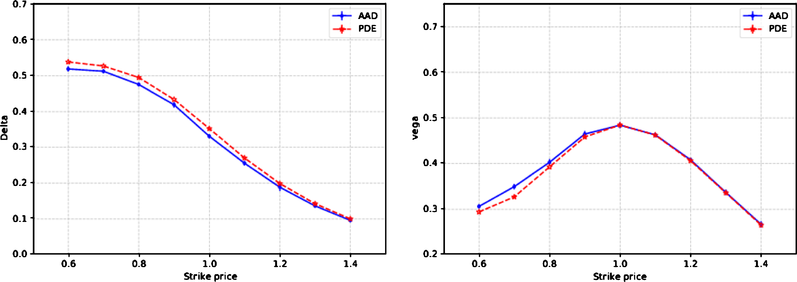
Table 1
Prices, Deltas and Vegas for the Bermudan-style option in (80) with three different strike values. The smoothening parameter in the call spread regularization (48) is δ = 0.005. The number of MC paths employed in the AAD approach is 400,000. The results are obtained with the setting (81) and (82). The MC uncertainty (in parenthesis) is computed using the binning technique of Capriotti and Giles (2010) with 20 bins for each set of simulations
| K = 0.9 | Price | Delta | Vega |
| AAD | 0.2012(2) | 0.415(3) | 0.456(2) |
| PDE | 0.20107 | 0.41423 | 0.45740 |
| K = 1.0 | |||
| AAD | 0.1396(1) | 0.337(2) | 0.486(2) |
| PDE | 0.13959 | 0.33588 | 0.48440 |
| K = 1.1 | |||
| AAD | 0.0941(2) | 0.258(1) | 0.463(2) |
| PDE | 0.09431 | 0.25635 | 0.46253 |
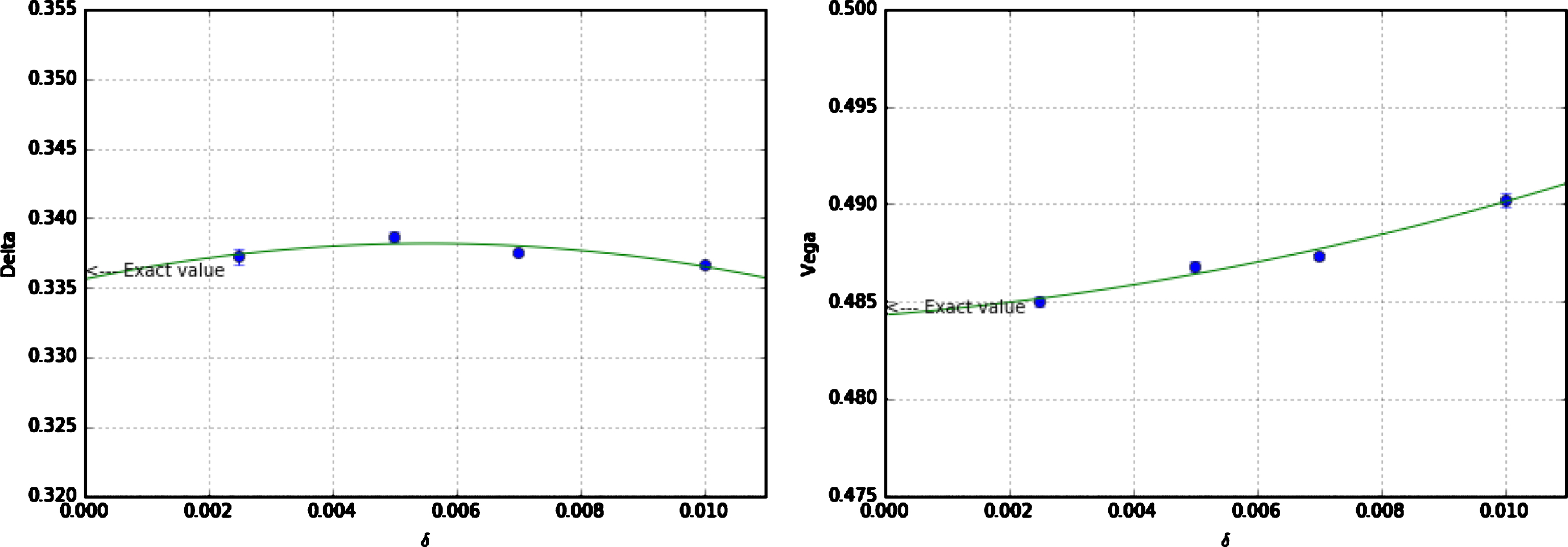
Here the smoothening parameter for the calculation of the Greeks, discussed in Section 3.1, δ = 0.005, was chosen as a reasonable compromise between variance and bias of the estimator. This is illustrated in Fig. 2, showing how for δ = 0.005 the bias introduced by the finite δ is of the same order of magnitude of the statistical uncertainty for the chosen computational budget, and is negligible for any practical application.
Fig.2
AAD Delta (left panel) and Vega (right panel) of the Bermudan-style option in (80) for K = 1 vs the smoothening parameter δ for the call spread regularization (48). The number of simulated paths is 3,000,000 for δ = 0.01 and is increased as δ is decreased in order to keep statistical uncertainties roughly constant. The results are obtained with the setting (81) and (82). The values in the graphs are fitted based on a quadratic polynomial function (green lines).
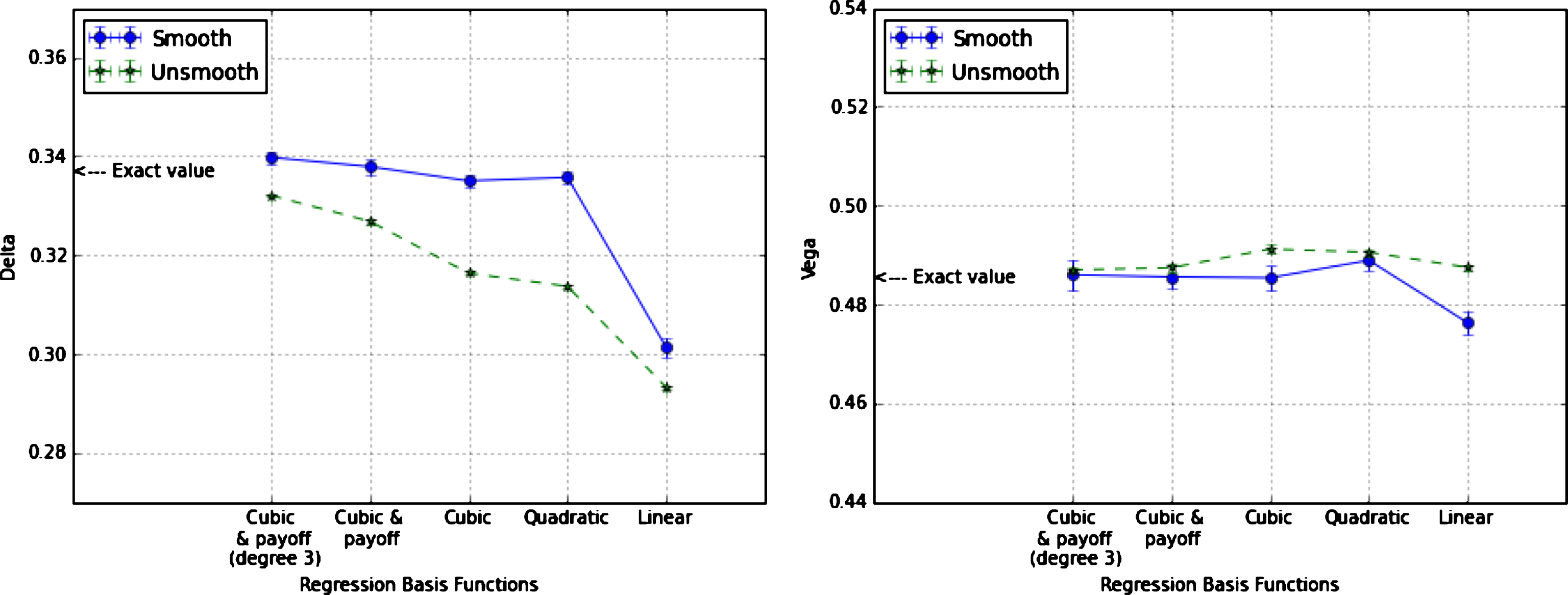
As discussed in Section 3.1, neglecting to smoothen out the exercise boundary, although common in the financial practice, introduces a bias in the computation of sensitivities because the exercise boundary is in general not optimal. This is illustrated in Fig. 3, in which we compare the Delta, with and without smoothening, for different choices of the basis functions. These results are obtained with the inputs (81) and (82). Here for Delta, the smoothened estimator turns out to be more accurate, especially when the exercise boundary obtained by regression is a less accurate approximation of the real one. However, it is difficult to establish a priori whether the unsmoothened estimator provides a smaller or a larger bias than the smoothened one. This is because the bias introduced by the lack of smoothening may be offset by the bias arising from the sub-optimality of the exercise boundary. This is illustrated in the right panel of Fig. 3 showing that for Vega the smoothened and unsmoothened estimators have a comparable accuracy. In any case, a consideration to keep in mind is that smoothening the exercise boundary is generally required to obtain stable second-order risk values.
Fig.3
AAD Delta (left panel) and Vega (right panel) of the Bermudan-style option in (80) for K = 1 as obtained with the unsmoothened and the smoothened estimators with the call-spread regularization (48) for five choices of the regression basis functions. The number of simulated paths is 1,000,000 with 20 bins and the smoothening parameter is δ = 0.005.
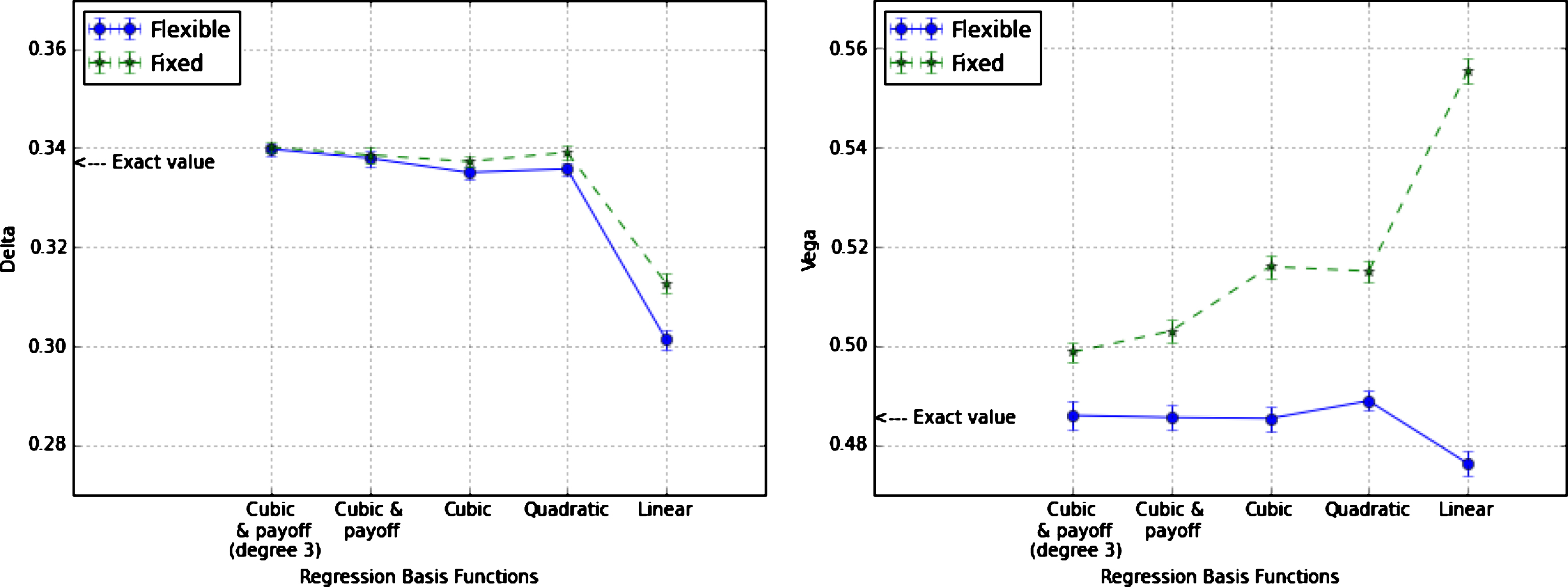
The quasi-optimality of the exercise boundary is also generally invoked among industry practitioners as a justification for neglecting the contributions to the sensitivities arising from the exercise boundary. Clearly, the quality of this approximation is dependent on the accuracy of the regression functions in reproducing the actual exercise boundary. This is illustrated in Fig. 4 where we plot Delta and Vega of the Bermudan-style option (80) for different choices of the regression basis functions. Here we compare the results obtained by the AAD algorithm, as described in Section 3.4, in the case where a) the exercise boundary is kept fixed, and b) when accounting instead for its contributions to the sensitivities. As expected, the difference between the two approaches vanishes as the regression functions become more accurate. However, as it is shown for the Vega, it can lead to a significant bias if a simple (e.g., linear or quadratic) representation of the exercise boundary is adopted.
Fig.4
AAD Delta (left panel) and Vega (right panel) of the Bermudan-style option in (80) for K = 1 as obtained by keeping the exercise boundary fixed (Fixed) and accounting instead for its contributions to the sensitivities (Flexible). The number of simulated paths is 1,000,000 with 20 bins and the call-spread smoothening parameter is δ = 0.005.
4.2XVA sensitivities
As another example, we compute the sensitivities of XVA (14) for the same option defined in Equation (80). Here, for simplicity, we assume that the hazard rate and the volatility are piecewise constants. The following results are obtained with the specifications (81) and (82). The XVA sensitivities with respect to some of the model parameters, namely the term structure of hazard rates of the counterparty and of volatilities of the underlying, obtained with the AAD algorithm described in Section 2.5 are compared with the ones obtained by standard bumping in Tables 2 and 3. As expected, the AAD sensitivities are in excellent agreement with those obtained by bumping with any discrepancies attributable to the bias of the finite-difference approach completely masked in this example by the MC uncertainties.
Table 2
The XVA sensitivities with respect to the piecewise volatility. The results are obtained with the setting (81) and (82). Both sets of the results are computed with 1,000,000 MC paths and 25 bins
| σ0 | σ1 | σ2 | σ3 | σ4 | σ5 | |
| AAD | 0.00298(1) | 0.00297(2) | 0.00294(1) | 0.00283(1) | 0.00271(1) | 0.00255(1) |
| Bumping | 0.00298(1) | 0.00297(2) | 0.00294(1) | 0.00283(1) | 0.00271(1) | 0.00255(1) |
| σ6 | σ7 | σ8 | σ9 | σ10 | σ11 | |
| AAD | 0.00236(1) | 0.00218(1) | 0.00201(1) | 0.00183(1) | 0.00165(1) | 0.001450(8) |
| Bumping | 0.00236(1) | 0.00218(1) | 0.00201(1) | 0.00183(1) | 0.00165(1) | 0.001450(8) |
Table 3
The XVA sensitivities with respect to the piecewise hazard rates. The results are obtained with the setting (81) and (82). Both sets of the results are computed with 1,000,000 MC paths and 25 bins
| λ0 | λ1 | λ2 | λ3 | λ4 | λ5 | |
| AAD | 0.03337(1) | 0.03336(2) | 0.03329(2) | 0.03306(3) | 0.03269(3) | 0.03218(3) |
| Bumping | 0.03337(1) | 0.03336(2) | 0.03329(1) | 0.03306(3) | 0.03269(3) | 0.03218(3) |
| λ6 | λ7 | λ8 | λ9 | λ10 | λ11 | |
| AAD | 0.03151(3) | 0.03074(4) | 0.02989(4) | 0.02893(4) | 0.02784(4) | 0.02669(4) |
| Bumping | 0.03151(3) | 0.03074(3) | 0.02989(4) | 0.02893(4) | 0.02784(4) | 0.02669(4) |
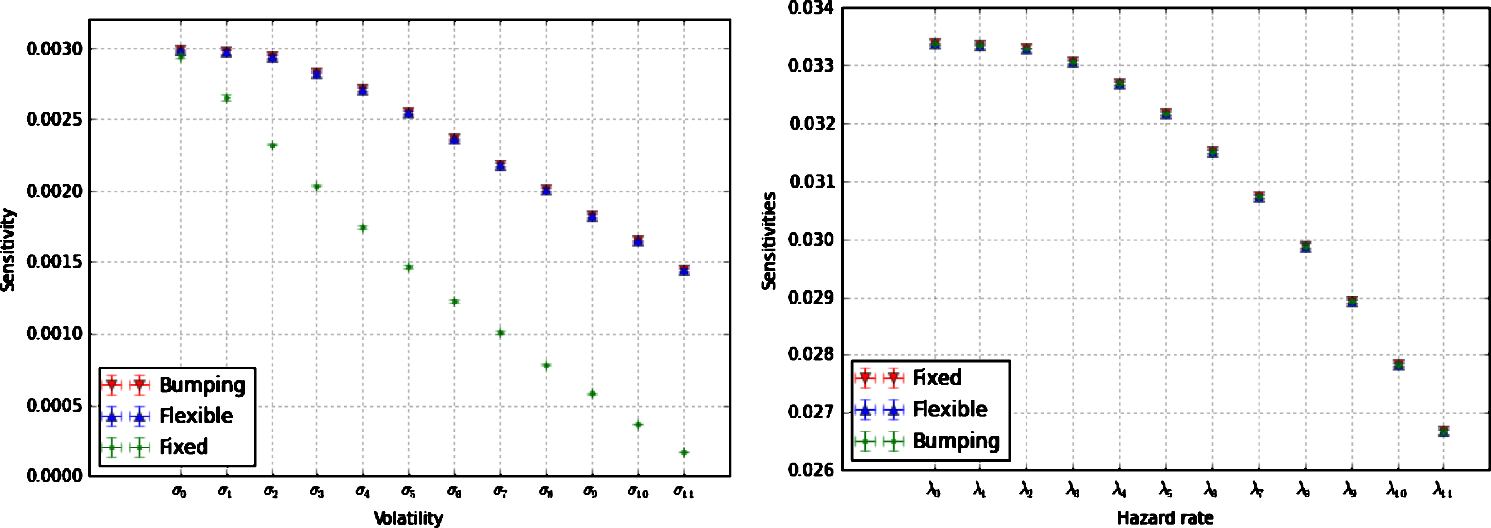
Similar to the case of Bermudan-style option Greeks, keeping the regression boundary fixed while computing the sensitivities, introduces a bias. However, for XVA, this issue is much more severe than in the case of the Bermudan-style option Greeks because no quasi-optimality argument can be invoked. As shown in Fig. 5, the volatilities sensitivities obtained by bumping and AAD keeping into account of the regression contributions are almost identical. Instead, the results of AAD keeping the regression coefficients fixed are remarkably different and, if utilised for risk management, would lead to significant mis-hedging. On the other hand, as expected, the XVA sensitivities with respect to the hazard rates are not affected by the contribution arising from the regression functions. This is because the hazard rates do not enter the computation of the portfolio value conditional on default, and hence do not appear in the regression parameters.
Fig.5
XVA sensitivities with respect to the piecewise volatility (left panel) and hazard rate (right panel), computed by AAD keeping into account of the contributions of the regression coefficients (Flexible), by AAD keeping the regression coefficients fixed (Fixed), and by finite-differences (Bumping). The number of MC paths is 1,000,000 and the number of bins is 25. The results are obtained with the setting (81) and (82).
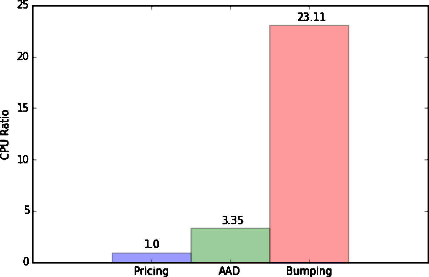
Finally, the remarkable computational efficiency of the AAD approach is illustrated in Fig. 6. Here we plot the cost of computing the XVA sensitivities with respect to the term structure of the counterparty hazard rate and the underlying volatility, relative to the cost of performing a single valuation. The calculation of the sensitivities by means of AAD can be performed in about three times the cost of computing the XVA value, that is, well within the theoretical bound (7). In contrast, the cost of bumping, for one-sided finite-difference estimators, is in general (1 + N) times the cost of as single valuation, where N is the number of model parameters, i.e., in this case over 20 times the cost of computing the value of the XVA.
Fig.6
Ratio of the CPU time required for the calculation of the XVA, and its sensitivities, and the CPU time spent for the computation of the XVA alone.
5Conclusions
We have shown how Adjoint Algorithmic Differentiation (AAD) can be utilised to implement efficiently the computation of sensitivities in regression-based MC methods. We have derived the AAD version of the celebrated least-square algorithms of Tsitsiklis and Van Roy (2001) and Longstaff and Schwartz (2001) and, by discussing in detail examples of practical relevance, we have demonstrated how accounting for the sensitivities contributions associated with the regression functions is crucial to obtain accurate estimates of the Greeks in XVA applications and for Bermudan-style options, especially when the exercise boundary is not particularly accurate. We have also shown how smoothening out the discontinuities associated with suboptimal exercise boundaries can lead in some situations to more accurate estimates of the sensitivities.
From a computational stand point, similarly to what was previously found in other MC and PDE settings, see e.g., Capriotti and Giles (2012); Capriotti et al. (2015), the proposed method allows the computation of the complete first-order risk at a cost which is at most four times the cost of calculating the value of the portfolio itself. This typically results in orders of magnitude of savings in computational time with respect to standard finite-difference approaches, thus making AAD an ever so indispensable technique in the toolbox of modern financial and insurance engineering.
Notes
1 In the following, for simplicity of notation, we will set N(0) =1.
2 Here and in the following, to keep the notation simple, we do not introduce different symbols for expectations and the respective sample averages.
Acknowledgments
It is a pleasure to thank Jacky Lee, for numerous useful discussions, and for a careful reading of the manuscript. We are also grateful to the anonymous referee for the feedback and comments. After completion of this manuscript we became aware of the work performed simultaneously by Antonov on a similar application of AAD to Callable Exotics, see Antonov (2016). The opinions and views expressed in this paper are uniquely those of the authors, and do not necessarily represent those of Credit Suisse Group.
References
1 | Andersen L. , Broadie M. (2004) . Primal-dual simulation algorithm for pricing multidimen-sional American options, Management Science 50: (9), 1222–1234. |
2 | Andersen L. , Piterbarg V. (2010) . Interest Rate Modeling, Volume I: Foundations and Vanilla Models, Atlantic Financial Press. |
3 | Antonov A. (2016) . Algorithmic Differentiation for Callable Exotics. SSRN: https://ssrn.com/abstract=2881992 |
4 | Broadie M. , Glasserman P. (1997) . Pricing American-style securities using simulation, Journal of Economic Dynamics and Control 21: (8), 1323–1352. |
5 | Broadie M. , Glasserman P. (2004) . A stochastic mesh method for pricing high-dimensional American options, Journal of Computational Finance 7: (4), 35–72. |
6 | Capriotti L. (2011) . Fast greeks by algorithmic differentiation, Journal of Computational Finance 14: (3), 3–35. |
7 | Capriotti L. , Giles M. (2010) . Fast correlation Greeks by adjoint algorithmic differentiation, Risk 23: , 79–85. |
8 | Capriotti L. , Giles M. (2012) . Algorithmic differentiation: Adjoint greeks made easy, Risk 25: , 92–98. |
9 | Capriotti L. , Jiang Y. , Macrina A. (2015) . Real-time risk management: An AAD-PDE approach, International Journal of Financial Engineering 2: (04), 1550039–1550070. |
10 | Capriotti L. , Lee S. J. (2014) . Adjoint credit risk management, Risk 27: , 92–98. |
11 | Capriotti L. , Peacock M. , Lee J. (2011) . Real time counterparty credit risk management in Monte Carlo, Risk 24: , 86–90. |
12 | Carriere J.F. (1996) . Valuation of the early-exercise price for options using simulations and non-parametric regression, Insurance: Mathematics and Economics 19: (1), 19–30. |
13 | Cesari G. , Aquilina J. , Charpillon N. , Filipovic Z. , Lee G. , Manda I. (2009) . Modelling, pricing, and hedging counterparty credit exposure: A technical guide. Springer Science & Business Media. |
14 | Crépey S. , Bielecki T.R. , Brigo D. (2014) . Counterparty risk and funding: A tale of two puzzles. CRC Press. |
15 | Friedman J. , Hastie T. , Tibshirani R. (2001) . The elements of statistical learning (Vol. 1). Springer, Berlin: Springer series in statistics. |
16 | Geeraert S., Lehalle C.A., Pearlmutter B., Pironneau O., Reghai A. (2017) . Mini-symposium on automatic differentiation and its applications in the financial industry. https://arxiv.org/abs/1703.02311 |
17 | Giles M.B. (2008) . Collected matrix derivative results for forward and reverse mode algorithmic differentiation. In Advances in Automatic Differentiation, 35–44. Springer Berlin Heidelberg. |
18 | Glasserman P. (2003) . Monte Carlo methods in financial engineering (Vol. 53). Springer Science & Business Media. |
19 | Griewank A. and Walther A. (2008) . Evaluating derivatives: Principles and techniques of algorithmic differentiation, Society for Industrial and Applied Mathematics. |
20 | Henrard M. (2014) . Adjoint algorithmic differentiation: Calibration and implicit function theorem, Journal of Computational Finance 17: (4), 37–47. |
21 | Joshi M. , Kwon O.K. (2016) . Least squares Monte Carlo credit value adjustment with small and unidirectional bias, International Journal of Theoretical and Applied Finance 19: (08), 1650048–1650064. |
22 | Lando D. (1998) . On Cox processes and credit risky securities, Review of Derivatives Research 2: (2-3), 99–120. |
23 | Leclerc M. , Liang Q. , Schneider I. (2009) . Fast Monte Carlo Bermudan greeks, Risk 22: (7), 84–88. |
24 | Longstaff F.A. , Schwartz E.S. (2001) . Valuing American options by simulation: A simple least-squares approach, Review of Financial Studies 14: (1), 113–147. |
25 | Savickas V. , Hari N. , Wood T. , Kandhai D. (2014) . Super fast greeks: An application to counterparty valuation adjustments, Wilmott 69: , 76–81. |
26 | Tsitsiklis J.N. , Van Roy B. (2001) . Regression methods for pricing complex American-style options, IEEE Transactions on Neural Networks 12: (4), 694–703. |
27 | Wilmott P. , Howison S. , Dewynne J. (1995) . The mathematics of financial derivatives: A student introduction. Cambridge University Press. |
28 | Xu W. , Chen X. , Coleman T.F. (2016) . The effcient application of automatic differentiation for computing gradients in financial applications, Journal of Computational Finance 19: (3), 71–96. |


