
Sensitivity and computational complexity in financial networks
Abstract
Determining the causes of instability and contagion in financial networks is necessary to inform policy and avoid future financial collapse.
In the American Economic Review, Elliott, Golub and Jackson proposed a simple model for capturing the dynamics of complex financial networks. In Elliott, Golub and Jackson’s model, the institutions in the network are connected by linear dependencies (cross-holdings) and if any institution’s value drops below a critical threshold, its value suffers an additional failure cost. This work shows that even in this simple model there are fundamental barriers to understanding the risks that are inherent in a network.
First, if institutions are not required to maintain a minimum amount of self-holdings, any change in investments by a single institution can have an arbitrarily magnified influence on the net worth of the institutions in the system. This implies that if institutions have small self-holdings, then estimating the market value of an institution requires almost perfect information about every cross-holding in the system.
Second, even if a regulator has complete information about all cross-holdings in the system, it may be computationally intractable to estimate the number of failures that could be caused by a small shock to the system.
1Introduction
The recent financial crisis and subsequent bailout have highlighted the need for a better understanding of the dynamics of financial networks. Indeed, the complexity of modern financial networks has been blamed for our collective failure to recognize the presence of serious risks in these systems. In this work, we show that even in extremely simple financialnetworks understanding the risk present in the system is computationally intractable in general – even in the presence of perfect information about all participants in the system. We hope that these insights will help regulators and policymakers to better understand the dynamics of financial networks.
Understanding an individual’s risk in a financial network is a difficult task, because an institution’s ability to fulfill its outgoing financial obligations is not a local property, i.e., it cannot be understood by examining a single individual in isolation. An institution’s ability to make its outgoing payments may depend on whether its incoming payments are made by its debtors, which in turn may depend on whether the incoming obligations are made to those institutions, etc. Thus each institution, acting without a global view of the network, cannot effectivelyunderstand its risk. Nevertheless, one might hope that a regulator, with a global view of the network could better understand the opportunities and risks inherent in the system. Even with a global view, the situation remains relatively complex. One complicating factor is the existence of cycles in the financial network, for example institution A may have obligations to institution B which has obligations to institution C, which in turn has obligations to institution A. The existence of these cyclical interdependencies has been put forward as one of the primary sources of complexity in financial networks. In this work, we will examine network dynamics in both cyclic (Theorem 1) and acyclic networks (Theorem 3). One of the driving forces in the study of financial networks is their ability to magnify risk: if an institution, A, defaults on its obligations to institution B, this may cause institution B to default on its obligations to institution C etc. The spread of risk through a financial network is known as financial contagion and has been carefully modeled and studied (Allen and Gale, 2000; Eisenberg and Noe, 2001; Gouriéroux, Héam, and Monfort, 2012; Acemoglu, Ozdaglar, and Tahbaz-Salehi, 2013; Glasserman and Young, 2014; Elliott, Golub, and Jackson, 2014). This work focuses on quantifying the ability of financial networks to amplify and conceal risk.
2Our contributions
In this work, we study two questions related to the stability of financial networks. First, we look at how sensitive market valuations can be to small changes in network structure. Second, we examine the computational complexity of determining how far a given network is from a massive failure. Throughout this work we use the network model put forward by Elliott (Golub, and Jackson, 2014). In this model, financial institutions own shares of underlying assets, and the institutions are connected by cross-holdings, which are modeled as linear dependencies. If an institution’s market value drops below a certain critical threshold, its value suffers a further discontinuous shock, modeling the effects of a loss of investor confidence, or the failure to pay everyday operating costs. See (Elliott, Golub, and Jackson, 2014) for an in-depth discussion of the interpretation and real-world validity of this model. The formal mathematical model is described in detail in Section 4.
Our first result (Theorem 2), shows that financial networks can be highly sensitive to small changes in their link structure. Concretely, we show that if a single institution changes a single cross-holding by ε, the market values of institutions in the system can change by as much as ε/2r, where r ≤ 1 is the minimum amount of self-holdings of the institutions in the network. The minimum self-holdings, r, is a measure of integration of the network, where r = 0 corresponds to a fully integrated network, and r = 1 corresponds to a network with no integration. This result shows that if each institution retains only, say, 5% self-ownership, a change in a single holding by ε can result in a 20ε change in an institution’s market value. This amplification is directly caused by cycles in the network, and in acyclic networks this type of magnification cannot occur (see Lemma 1). Our bounds are essentially tight, and Theorems 1 and 2, show that the true sensitivity is in fact Θ (ε/r). This sensitivity magnification has many consequences. First, it means that in order to estimate market values of institutions within the system, all cross-holdings need to be known to an extremely high degree of precision. Investors or regulators who wish to calculate market values can be extremely far off if even a single cross-holding in the network remains unknown to them. Second, because small changes in a single institution’s investments can have large effects on market values throughout the system, this indicates a potential for extreme instability in the system as a whole; the small portfolio changes in one institution can have a drastically magnified effect market values of other institutions, and so small changes by a myopic institution could topple even seemingly stable institutions. Third, this extreme sensitivity means that calculating market values in a privacy-preserving manner can be extremely difficult (Narayan, Papadimitriou, and Haeberlen, 2014). This is the flip-side of the first point, in order to calculate market values for institutions in the system, all the interbank holdings need to be known with high precision, which means that revealing market prices has the potential to reveal extremely detailed information about each institution’s interbank holdings. Our second result addresses the question of how well a regulator can assess the stability of a network. Suppose a regulator or oversight agency is presented with a network in which every bank is solvent, and suppose the regulator believes that the underlying assets cannot drop in value by more than some fixed amount d. What is the maximum number of failures that can be caused by a drop of this size in asset values? We emphasize that in this scenario, the regulator has complete information about the entire structure of the financial network, and the only uncertainty is in which specific assets may decline in value. We show calculating the number of institutions that can fail in a network is NP-Hard. In particular, we show that is as hard as calculating the maximum balanced clique in a bipartite graph (Theorem 3). The maximum balanced bipartite subgraph (BCBS) problem is NP-hard (Gary and Johnson, 1979; D.S. Johnson, 1987), and there is evidence that it is even hard to It is known that if 3-SAT is not in DTIME (2n3/4+ε) for some ε, then there is no polynomial time algorithm for calculating the maximum balanced clique to within a factor of 2(logn)δ for some δ > 0. Feige and Kogan (2004) go further, conjecturing that there is no polynomial time algorithm to approximate the maximum balanced bipartite clique to within a factor of nδ for some δ > 0. This would imply that there is no polynomial time algorithm that can even estimate the maximum number of failures caused by a drop in asset values of a given magnitude to within a factor of nδ in a network with 2n institutions. In particular, this means that there are financial networks where stress testing (which is inherently computationally feasible) cannot hope to even approximate the magnitude of collapse that could be caused by some bounded drop in assetvalues. Unlike our first result, which crucially relies on cycles in the network, this result holds even in acyclic networks: even when there are no cycles it is computationally intractable to estimate the maximum number of failures that could be caused by a bounded drop in asset values. This complexity arises not from cycles, but from the nonlinear dynamics that occur when a bank drops below its critical threshold value.
3Previous work
Many different models have been proposed to study financial networks, and specifically models of stability and contagion.
Allen and Gale (1998) considered a model consisting of depositors and banks. Depositors deposit their money in the banks, and the banks must choose between making short-term investments or long-term investments. This model has three time periods, t = 0, 1, 2. At t = 0, investments are made, at t = 1 short-term investments pay off, and depositors choose whether to withdraw their money, and at time t = 2 long-term investments pay off. The banks’ investment strategies then depend on the probability that depositors withdraw their money at time t = 1. In a follow-up work Allen and Gale (2000) introduced a network component, where banks can exchange deposits with each other in an effort to mitigate risk, and they showed simple contagion effects in this model.
Acemoglu, Ozdaglar, and Tahbaz-Salehi (2013) build on Allen and Gale’s 3 time-step model. At time t = 0 banks can make a short-term investment, a long-term investment or loan money to other banks. Long term investments yield a fixed return at t = 2. Long term investments that are liquidated at t = 1 receive a return that is randomly distributed between two values. Banks whose investments returned the lower of the two values were said to have received a shock. Acemoglu, Ozdaglar and Tahbaz-Salehi considered how two extremal types of networks serve to propagate these shocks. They considered the ring (where each bank only has debts to its two neighbors) and the complete network where each bank’s debts are spread to all other banks, as well as all convex combinations of these two. They showed that if the magnitude of the shocks are small then the complete network is more stable and resilient than the ring, and if the magnitudes of the shock are large enough then both the ring and complete networks are the least stable networks, thus the complete network exhibits a phase transition, moving from the most stable to the least stable network as the magnitude of the shocks increase.
Eisenberg and Noe (2001) developed a very simple and appealing network model where each bank has cash reserves and fixed debts to other banks. Eisenberg and Noe’s work focused on showing that (under some basic restrictions on the network) there is always a unique clearing vector (indicating how much of its debts each bank pays to its creditors), and they gave a linear program and simple iterative algorithm for calculating this clearing vector and hence the equilibrium valuation of each bank.
Gai and Kapadia (2010) considered a modification of Eisenberg and Noe’s network model, forcing all incoming edges to have the same weight, but allowed banks to have additional illiquid assets. Gai and Kapadia then considered the question of how a single bank failure propagates through a network. For this analysis, they considered different models for generating the underlying graph topology, and plotted contagion effects for different network models characterized by their degree distribution. They found that a single large shock could have devastating effects on the network, but that this was highly dependent on where in the network the shock hit.
Gouri'eroux, H'eam, and Monfort (2012) considered a model that allows interbank investment via shares (like (Elliott, Golub, and Jackson, 2014)) and lending or insurance (like (Eisenberg and Noe, 2001)). Unlike (Eisenberg and Noe, 2001)). Unlike (Elliott, Golub, and Jackson, 2014), they do not introduce discontinuous failure costs. Gourieroux, Héam and Monfort extend Eisenberg and Noe’s uniqueness results to show that (under mild constraints on the network) this extended model has a unique equilibrium value for all institutions. They then examined the effects of exogenous shocks on the network (i.e., drops in asset values) using synthetic data and data obtained from the French banking sector.
Morris (2000) studied contagion in local interaction systems. In that model, each node represents a player, and each player engages in a local game with each of its neighbors. Morris focused on the case where each player has a binary strategy space, {0, 1}, and there is a global 2 × 2 payoff matrix, such that for each edge in the graph, the two neigboring players receive a payoff according to this global payoff matrix. In that model, a strategy is said to be “contagious,” if it can spread from a finite set of players to an infinite set of players by the best-response dynamics of the underlying local game.
The notion of failure cascades and contagion have also been studied in the computer science literature by Blume et al. (2011), Blume et al. considered general cascades in graphs where the edges were unweighted and a node was said to fail if some critical threshold of its neighbors failed. By choosing all edges to have equal weight, and choosing each institution’s failure threshold carefully, the failure model of (Elliott, Golub, and Jackson, 2014) can be made to overlap with this general network failure model.
In this work, we use the model of Elliott (Golub, and Jackson, 2014). In this model, institutions can own shares in each other, or in “primitive assets” that have intrinsic value outside of the network. The model is explained in detail in the next section. Elliott, Golub and Jackson introduced this model to help analyze and understand contagion effects in networks. Because a cascade of collapse requires an initial failure, Elliott, Golub and Jackson began by showing that the weakest institution can never be made strictly more stable by any fair trade between the institutions. Next they examined the contagion dynamics in a wide class of networks parametrized by “integration” and “diversification.” Integration increases as institutions in the network increase their inter-network holdings, i.e., integration increases as the percentage of each institution owned by shareholders external to the network decreases. As integration increases, the institutions’ fates are more closely tied together. Diversification measures how risk is spread within the network. Diversification increases as institutions increase their number of cross-holdings. Neither integration nor diversification have strictly positive or negative effects on network stability, but instead have slightly more complex non-monotonic effects.
The notion of computational complexity has been studied in the context of financial products by Arora et al. who showed that banks can create derivatives that are computational intractable to price accurately (Arora et al., 2010, 2011). The result of Arora et al. crucially relies on the information asymmetry between the institution the seller (who creates the derivatives) and the buyer who only sees their resulting composition. Braverman and Pasricha (2014) show that even in the full information setting pricing compound options is PSPACE complete.
4Model
We use the model put forward by Elliott (Golub, and Jackson, 2014). In this model there are n financial institutions, these can be viewed as countries, banks or private firms, and m underlying assets, that can be viewed as any object or project with intrinsic value. The financial institutions own shares of the underlying assets which impart value into the system. The values of the institutions themselves are interconnected via a network (modeled as a weighted, directed graph). The interdependencies (cross-holdings) between the institutions are modeled as simple linear dependencies. These linear cross-holdings can model simple equity stakes (one institution owning shares in another) or they can be viewed as an approximation of more complicated debt contracts between the institutions (see (Elliott, Golub, and Jackson, 2014, Section 2.5) for a more thorough discussion of the validity and generality of this model).
Although institutions invest in one another, all value in the system originates from the underlying assets. The price of asset k is denoted by pk, and we use Dik ≥ 0 to denote the percentage of asset k owned by institution i. The n × m matrix of ownership is denoted by D = (Dik).
We define C = (Cij) to be the n × n matrix indicating the cross-holdings of institutions. Thus institution i owns a Cij fraction of institution j. It will be be useful to view the network of cross-holdings as a directed graph with n nodes representing the financial institutions, and an edge from institution j to i of weight Cij whenever Cij > 0. Following (Elliott, Golub, and Jackson, 2014), we set Cii = 0 for all i. Now, ∑iCij is the fraction of institution j that is owned by institutions external to j. The remainder, the amount of self-ownership, is denoted by
As noted by Brioschi (Buzzacchi), this type of model introduces two types of valuations, the equity valuation (
(1)
In matrix notation, this becomes
This equity valuation significantly overvalues the institutions. In particular, we can see that
To find an institution’s market value, we must scale the institution’s equity value by the percent stake it has in itself, thus the market value of institution i is
(2)
The matrix C is column sub-stochastic because column i sums to
5Sensitivity
Our first result concerns concerns the sensitivity of valuations to small changes in the structure of the network. Suppose a single institution shifts its holdings by a small quantity, ε, how much can this small change affect the market valuations in the network? This question is motivated by questions about network stability, and the possibility of privacy-preserving oversight. If small changes in network holdings can lead to large changes in the market values of the institutions, this indicates a fundamental instability in the financial network. Additionally, if small changes in interbank holdings can lead to large changes in market values, then any attempt at financial oversight must incorporate all the interbank holdings to a high degree of accuracy in order to predict market values.
A high sensitivity also has implications towards privately computing network statistics. Flood et al. (2013) proposed using tools from differential privacy (Dwork, 2006; Dwork et al., 2006) to provide a means of computing global network characteristics while preserving the privacy of each individual institution’s holdings. A high sensitivity implies a worse trade-off between privacy and accuracy when calculating network statistics.
We begin our sensitivity analysis with a simple observation: if the total value of the underlying assets is
Fig.1
An ε change results in an
![An ε change results in an ε∥p→∥ change in market values. Banks are in blue, external shareholders are in green, and the asset is
shown in red. In this example Dp→=[10], and C = 0. Thus v→=[10]. Changing C to C˜=[0ε00] leads to a valuation of v→˜=[1−εε]
, thus the market valuation of B2 changes by ε∥p→∥.](https://content.iospress.com:443/media/af/2016/5-3-4/af-5-3-4-af166/af-5-af166-g001.jpg)
Throughout this section, we use r (for “reserve”) to measure the fraction of each institution held by investors outside the system.1 We define
5.1Sensitivity in acyclic networks
We begin by noting that in the acyclic case, there is a strong bound on each institution’s equity valuation, i.e., the equity valuation cannot be too much larger than the market valuation.
Lemma 1. If the banking network has no cycles, then every institution’s equity valuation is at most
Proof. Organize the financial network into layers, so that each institution only owns shares of institutions at lower layers. Thus institutions at level 1 do not have any cross-holdings, they only own the underlying assets. This means that the incoming edges to level one carry a total weight of at most
Now each institution’s equity value is the sum of the values on all incoming edges. Since outgoing edges carry a value that is a percentage of equity value, the sum of the values on each institution’s outgoing edges is at most the sum of the values on its incoming edges. (For real institutions the outgoing sum will be strictly less because the reserve rate r > 0, but for the fictitious institutions it can be exactly equal.)
Now, the sum of the values coming into layer 1 is at most the sum of the assets,
Corollary 1. If the banking network is acyclic, and one edge changes by at most ε, then no institution’s market value can change by more than
Proof. Since each institution’s equity value is at most
5.2Sensitivity in general networks
In this section, we explore how much the market valuations can change when one bank changes its holdings by a small amount in the presence of cycles in the network graph. We begin by showing an upper bound on the change in market valuations that depends on the minimum self-ownership (
Theorem 1. If
Proof. Let
Now, we notice that
Because money is never created or destroyed, we have
Thus we have
Thus we immediately get the bound
Since
The multiplicative bound of ε/r in Theorem 1 is much weaker than the bound of ε in the acyclic case (Corollary 1), as the minimum self-holdings approaches 0, this difference tends towards infinity. This discrepancy is not a limitation of our proof, but arises as an artifact of the effect that holdings cycles can have on the equity (and market) valuations of the institutions in the network. In Theorem 2 we show that there exist networks where changing a single institution’s holdings by ε results in a change of
Theorem 2. There exist networks where
Proof. We exhibit an initial network in Fig. 2 and its perturbation in Fig. 3.
Fig.2
The initial configuration, banks are in blue, external shareholders are in green, and the asset is shown in red.
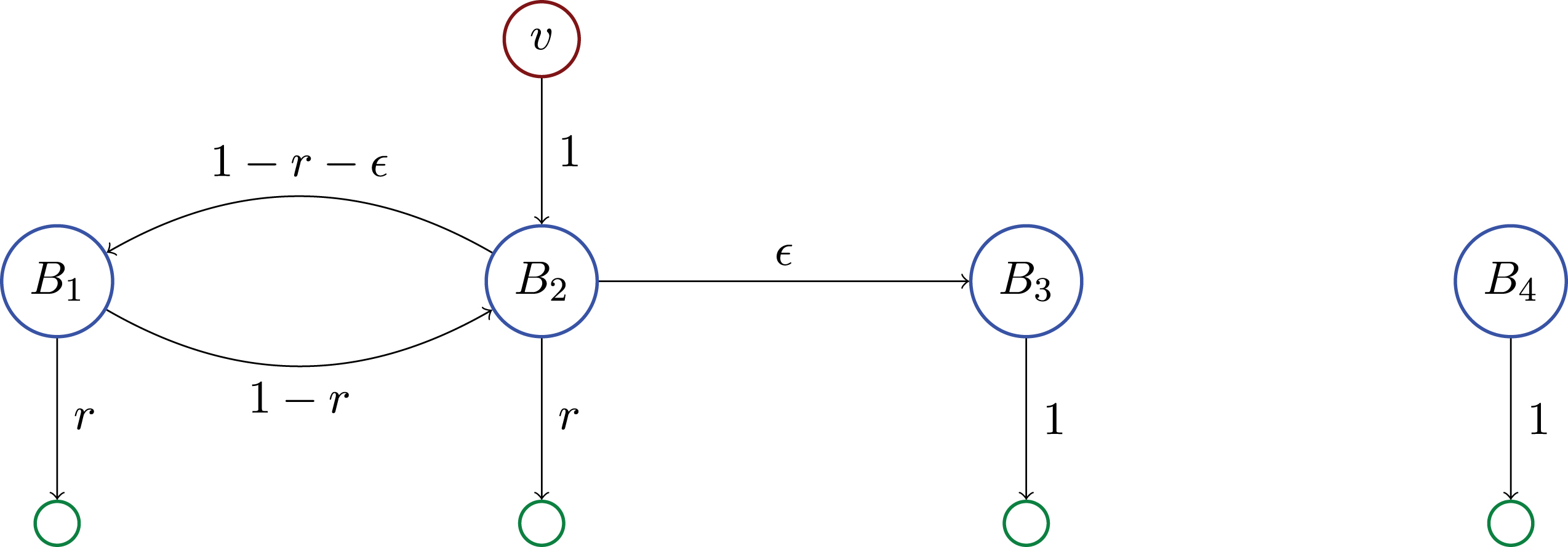
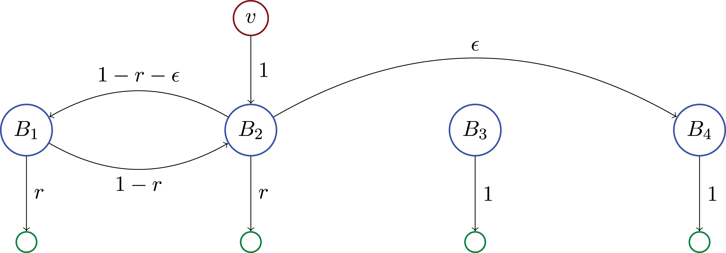
Fig.3
The perturbed configuration, where one link of weight ε has been moved from B3 to B4.
In Fig. 2, the equity values for the banks satisfy
So
Thus the market valuation of B3 is εB2 which is at least
If the link from B2 → B3 were moved to B2 → B4 (as in Fig. 3) then B3’s value drops to zero and B4’s value increases to εB2.
Thus the change in ℓ1 norm of the market valuations between the two situations is at least
Writing this in matrix notation, we have
Note that increasing one link by ε and decreasing another by ε is actually a change in 2ε in the
The type of equity amplification necessary for the lower bound in Theorem 2 cannot happen in an acyclic network (see Corollary 1).
Now, we compare the upper and lower bounds on sensitivity. We have an upper bound of
• For any ε, δ > 0, there exists an r with0 < r < 1 and a network with minimum reserve r such that a change in edge weights of ε can lead to a change in market valuations of at least (1 - δ) 2. Thus the upper bound cannot be decreased below 2.
• For any r, δ, with 0 < r < 1, and 0 < δ there exists an ε with 0 < ε < 1 and a network with minimum reserve r such that a change in edge weights of ε can lead to a change in market valuations of at least
Together, these show that the upper bound cannot be decreased below
6Bank failures
6.1Losses caused by failure
The model of (Elliott, Golub, and Jackson, 2014) includes a notion of “failure,” whereby institutions whose market value drops below a certain critical threshold suffer a further (discontinuous) loss in market value. These discontinuous penalties capture the notion that if an institution cannot pay its operating costs, it may see a further drop in revenues. Similarly, if confidence in the institution is shaken, and its debt rating is downgraded, it may see spike in the cost of capital, and hence see a further drop in value.
These discontinuous penalties are operationalized by a threshold value
Defining
(3)
Compare Equation 3 to the linear system given by Equation 2. The introduction of non-linear terms into the model adds significant complexity to the dynamics of the system, and can lead to failure cascades. One of the primary goals of (Elliott, Golub, and Jackson, 2014) was to characterize what network features affect the likelihood and severity of failure cascades.
6.2Overview of our complexity results
Suppose a regulator has complete information about a financial network, including all cross-holdings and the prices of all underlying assets. Further, suppose that at equilibrium, this network has no failures. If the regulator believes that tomorrow, asset prices may drop by some fixed amount d, (i.e., the sum total of asset prices may drop by d, but the exact drop of each asset price is unknown), what is the maximum number failures that could occur as a result of this drop? In other words, tomorrow, when the new equilibrium is calculated based on the new, lower, asset prices, what is the maximum number of banks that could have failed?
Our primary result is that the introduction of discontinuous failure costs increases the computational complexity of calculating basic network dynamics. If the complete network, as well as the price of all underlying assets is known, then the number of failures can be computed efficiently (Elliott, Golub, and Jack-son, 2014, Section 3.2.3). If, on the other hand, there is some uncertainty in the prices (or future prices) of the underlying assets, calculating the maximum number of failures that could occur in the network is computationally intractable.
Thus we address the following question: given a stable network (where no banks have failed), if the total prices of the assets drop by some small amount, what is the maximum number of failures that occur at equilibrium? One potential complication is that in networks with discontinuous failure penalties, there may not be a unique equilibrium, and hence the number of failures may not be uniquely defined. To address this, for any fixed set of asset prices, we use standard practice and only consider the “best-case” equilibrium (the one with fewest failures). On the other hand, we consider the worst drop in asset prices (i.e., the drop in asset prices that causes the most failures in its best-case equilibrium). Thus the “maximum” number of failures means the maximum over all bounded drops in asset values, of the minimum number failures that could occur at this each fixed drop in asset values (i.e., the minimum over all equilibria at these new, lower values). We discuss the issue of multiple equilibria in more detail in Section 6.3.
In real-world financial networks, regulators, as well as the institutions themselves routinely perform “stress-tests” to assess the robustness of the network to financial shocks. Our results indicate that there are financial networks where no (computationally feasible) stress test, will ever be able to even approximate the maximum number of failures that could occur from some small shock to the system.
Note, however, that our results are not probabilistic, in the sense that we do not model the probability of a specific drop in asset prices, instead we just impose a bound on the magnitude of the total drop in asset values. Without assigning probability distributions to the asset prices, we cannot assess the probability that such a cascade could occur, only that it is feasible. Thus our question is whether there exists a small specific drop in asset prices that could cause a huge failure cascade – whether this drop is probable is outside the scope of our model. Thus, if a stress-test could accurately model the probability distribution of asset prices, it may be able to assess the likely number of failures caused by a shock to the system, but any computationally feasible stress test will not be able to identify whether a small (but possibly unlikely) shock to the system could cause a far greater failure cascade.
6.3Multiple equilibria
When discontinuous failure penalties (
Fig.4
Banks are in blue, external
shareholders are in green, and the asset is shown in red. In this example
![Banks are in blue, external
shareholders are in green, and the asset is shown in red. In this example Dp→=[1001], and C=[012120]. If
v_i=2, and bi = 1, then two equilibria are: v→=[11], and v→=[00]](https://content.iospress.com:443/media/af/2016/5-3-4/af-5-3-4-af166/af-5-af166-g004.jpg)
In a network with multiple equilibria, we can talk about the “best-case” equilibrium (the one with the fewest failures) and the “worst-case” equilibrium (the one with the most failures). As in (Elliott, Golub, and Jackson, 2014), we focus on the best-case equilibrium, thus when we refer to the “the number of failures” we mean the number of failures in the best-case equilibrium.
6.4The Balanced Complete Bipartite Subgraph (BCBS) problem
Our hardness result is based on the hardness of finding a maximum balanced clique in a bipartite graph. This is known as Balanced Complete Bipartite Subgraph (BCBS) problem.
Definition 1 (BCBS). Given a bipartite graph G = (V1, V2, E) with |V1| = |V2| = n, the Balanced Complete Bipartite Subgraph (BCBS) problem is to find the largest integer K such that there exists sets C1 ⊂ V1 and C2 ⊂ V2 with the properties that |C1| = |C2| = K, and the induced graph on C1 ∪ C2 is a complete bipartite subgraph of G.
The BCBS problem is known to be NP-hard (Gary and Johnson, 1979; D.S. Johnson, 1987). This provides strong evidence that there is no scalable algorithm that it that can find the size of the maximum balanced clique in a bipartite graph.
In fact, there is significant evidence that even approximating the size of the largest balanced clique is hard. Feige showed that for some δ > 0 it is Random 3-SAT hard to approximate BCBS to within a factor of nδ (Feige, 2002, Theorem 3).
Feige and Kogan showed that if BCBS can be approximated to within a factor of 2(logn)δ for every δ > 0 then 3-SAT can be solved in time 2n3/4+ε for every ε > 0 (Feige and Kogan, 2004, Theorem 1.3).
Feige and Kogan go on to conjecture that for some δ > 0, there is no polynomial-time algorithm to approximate BCBS to within a factor of nδ (Feige and Kogan, 2004, Conjecture 1.1).
Our primary hardness result shows that there are networks where calculating the maximum number of bank failures that can result from a small shock is equivalent to solving the BCBS problem. Thus there are financial networks where even approximately estimating the number of bank failures that can result from an arbitrarily small drop in asset prices is a computationally intractable problem.
6.5The complexity of calculating the maximum number of failures
In this section, we give our main result concerning the computational complexity of estimating themaximum number of failures that can occur given a small drop in values of the underlying assets.
In particular, this hardness result applies finding the number of failures that occur at equilibrium when the institutional cross-holdings are fixed, and completely known, but there is some small uncertainty in the prices of the underlying assets.
In the situation that the cross-holdings and the assets are fixed, it is straightforward to calculate the market values of the institutions at equilibrium (Elliott, Golub, and Jackson, 2014, Section 3.2.3). Note that the network we construct is acyclic.
Theorem 3. For every bipartite graph G on 2n nodes, and every ε > 0, For every bipartite graph G on 2n nodes, and every ε > 0, there is a financial network with Ω (n) institutions, and a d > 0 such that computing the maximum number of institutions that could fail problem in G.
Proof. Let ℓ>0 be any integer.
Our starting point is the following hardness result for the BCBS problem. Given an n × n balanced bipartite graph G, it is hard to decide whether the largest balanced bipartite clique size in G is at least K × K or at most K/g × K/g for some gap function g. For instance, g = 2(logn)δ under the assumption that 3-SAT ∉DTIME (2n3/4+ε) for someε > 0.
Given an n × n balanced bipartite graph G, we will construct a financial network with (2 + ℓ) n institutions such that if G has a balanced bipartite subgraph of size K, then a drop in asset prices by Kε can cause at least (2 + ℓ) K failures. On the other hand, if the largest balanced bipartite then a drop in asset prices by Kε can cause at least (2 + ℓ) K failures.
This shows that estimating the maximum number of failures induced by a fixed drop in asset prices is at least as hard as estimating the size of the maximum balanced bipartite clique. Without loss of generality, we assume that every vertex in G has degree at least K.
Let D denote the maximum degree of any vertex in G. Let 0 < ε < 1 be an arbitrary parameter, and let 0 < r < 1 denote the minimum amount of self-holdings of the institutions in the network we are constructing. (The reduction will hold for any choices of 0 < ε, r < 1.)
For each node in the graph G, we will associate a financial institution. Let institutions 1, …, n correspond to the left-hand nodes of G, and institutions n + 1, …, 2n correspond to the right-hand nodesof G.
We will also generate n underlying assets, labelled
Define
For 1 = 1, …, n let
This financial network has the following properties:
1 If j > n and d of bank j’s neighbors fail, i.e., d of the assets ai (i ∈ Γ (j)) drop in value by ε, then bank j will fail.
2 If j > n and the total drop in value of bank j’s neighbors is less than
Now, we examine the properties of this system when the assets are allowed to drop in price by total amount dε. A drop of dε can always cause d institutions on the left-hand side of the network to fail, simply by dropping the value of each of their assets by ε.
What happens if the price drop is not concentrated among exactly d assets? Let t denote the number of assets that drop in value by at least ε. If t < d, then at least tε from the “shock budget” of dε was used to lower the price of these t assets, which leaves a budget of (d - t) ε remaining. Now, consider how much this drop can affect one of a right-hand institutions, j. Even if this drop is concentrated entirely among the left-hand neighbors of j, the drop j feels is at most
Now, suppose there is a biclique of size K in G. If d = K, then causing d failures among the left-hand members of this biclique will cause d = K failures among the right-hand members.
On the other hand, suppose the largest biclique is of size
Thus in the “yes” case (G has a biclique of size K) we can cause at least K right hand failures with a failure budget of Kε. In the “no” case (the largest biclique in G is of size
Now, to amplify this discrepancy, we add a chain of ℓ institutions connected to each right hand institution. Thus for every right-hand institution, bi, it will have a chain of institutions
Fig.5
There are n assets,
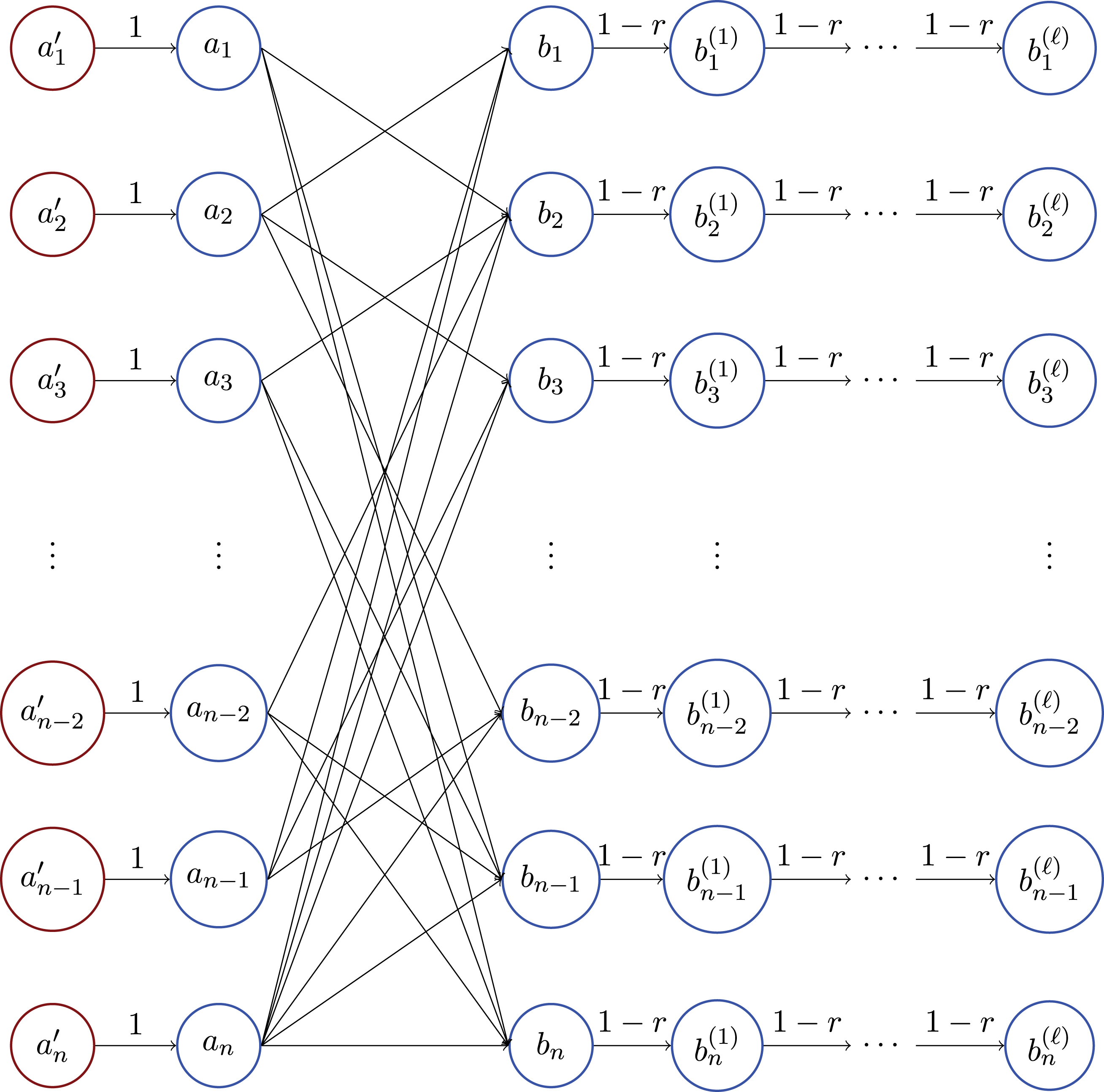
This new network has (ℓ +2) n banks, and has the following properties. Given a failure budget of Kε, if the largest balanced clique in G is a K × K, a drop in value by Kε causes at most (2 + ℓ) K, but if the largest biclique is of size
Note that when the gap, g = nδ, choosing ℓ = poly (n), we obtain a gap of ((ℓ +2) n) δ′ for some δ′ < δ.
Applying a result of Feige and Kogan (2004), we obtain the following Corollary.
Corollary 2. If 3-SAT ∉DTIME (2n3/4+ε) for some ε > 0, then there exists a δ > 0 such that there is no polynomial time algorithm that can calculate the maximum number of failures in a financial network caused by a drop in asset prices of dε to within a factor of 2(logn)δ′ for some δ′ > 0.
7Conclusion
This work highlights two distinct sources of instability in financial networks, instability arising from fluctuations in cross-holdings and instability arising from fluctuations in asset prices. More specifically, we show that there are networks where small fluctuations in cross-holdings or asset prices can have striking consequences, and these consequences have numerous implications.
Our first result (Corollary 1, Theorems 1, 2) shows that the effect of small changes in cross-holdings is strongly tied to the integration of the network. In highly integrated networks small changes in cross-holdings can have potentially unbounded effects on market valuations, while in networks with low integration, changes in cross-holdings have more tightly bounded effects on the market values of the institutions in the network. These results can be interpreted in many ways. From a regulatory perspective, in a highly integrated network, any regulator must know the entire cross-holdings network to a very high degree of accuracy in order effectively understand the market values of the institutions. From an institution’s perspective, small changes in investment by individual institutions can have their effects greatly magnified throughout the network. From a predictivity perspective, if one wishes to forecast market values into the future, any small forecasting uncertainty in the cross-holdings can have enormous effects on the (predicted) market values of the institutions. From a privacy perspective, institutions cannot maintain any privacy in their investment portfolios without compromising the ability of outsiders (e.g. other institutions, outside investors or regulators) to calculate the market value of the institutions. These problems arise only in highly integrated networks (Theorem 1), and they can all be mitigated by imposing a cap on integration. If institutions are required to maintain some fixed percentage of their ownership outside of the network, the sensitivity to changes in cross-holdings can be drasticallyreduced.
Our second result shows that small changes in the prices of the underlying assets can have unpredictable effects on the number of failures in the system. Specifically, we show that there are networks where it is computationally intractable, even with perfect information about the cross-holdings, to estimate the number of failures that can occur after some small drop in asset prices. This result too can be interpreted from different perspectives. This result implies that a regulator (with perfect information about the network cross-holdings) who believes there may be some bounded fluctuation in asset prices cannot be expected to distinguish a network where these fluctuations cause a small number of failures, from a network where fluctuations of the same magnitude can cause a massive number of failures. Institutions face the same computational challenge. An institution may wonder whether its investment portfolio will protect it from a bounded shock in asset prices, and our results show that even with complete information about the investments of all other agents in the system, it may be infeasible to determine whether a specific portfolio is safe.
Previous works have imposed specific probabilistic models on fluctuations in asset prices, and for a given probabilistic model the number of failures can usually be estimated. But what if the model is incorrect (e.g. the asset prices do not fluctuate independently)? Our results show that there are situations where changes in the distribution of fluctuations (but not their overall magnitude) can have huge and unpredictable effects on the number of failures.
Moving forward, it is an important research question to understand what constraints on the network will allow institutions and regulators to perform these stability analyses.
Appendices
Appendix
A. A flow model of the system
It is often instructive to create a stochastic matrix representing the system, which models money flowing through the network.
There are n financial institutions, and we introduce n addition entities, the “shareholders.” In this model shareholder i owns a
Initially, the banks are assumed to have some intrinsic value
The 2n × 2n matrix A allows us to view the market valuations of each institution as the steady state of a dynamical process. Money flows into the system from the underlying assets, and at each time step, the value residing in each financial institution is distributed to its stakeholders according to their stake. This process terminates when all the money in the system (coming from the underlying assets) has been distributed to the external shareholders. Algebraically, this process can be viewed as follows: given a vector
(4)
Throughout this work, we will use the standard operator norm for a matrix (in the L1 sense),
Because the columns of A sum to one, we have
(5)
Lemma 2.
If C is a matrix with ∥C ∥ <1, then I - C is invertible and
Proof. First, note if
Then, the result follows just as in the scalar case: Letting
This leads to the closed formula used in (Elliott, Golub, and Jackson, 2014):
(6)
Notes
1 The reserve, or self-holdings, can be viewed as the amount of an institution that is not sold, or is held by private shareholders, who retain complete ownership of themselves. These private shareholders buy shares of institutions in the network, but no entity in the network owns shares of the private shareholders.
References
1 | Acemoglu D., Ozdaglar A., Tahbaz-Salehi A., (2015) . Systemic risk and stability in financial networks. The American Economic Review 105: (2), 564–608. |
2 | Allen F. , Gale D. , (1998) . Optimal Financial Crises. In: The Journal of Finance 53: (4), pp. 1245–1284. DOI: 10.1111/0022-1082.00052 |
3 | Allen F. , Gale D. , (2000) . Financial Contagion. In: Journal of Political Economy 108: (1), pp. 1+. ISSN: 00223808. DOI: 10.1086/262109 |
4 | Arora S. , et al. (2010) . Computational Complexity and Information Asymmetry in Financial Products. In: ICS. Tsinghua University Press, pp. 49–65. |
5 | Arora S. , et al. (2011) . Computational Complexity and Information Asymmetry in Financial Products. In: Commun. ACM 54: (5), pp. 101–107. ISSN: 0001-0782. DOI: 10.1145/1941487.1941511 |
6 | Blume L. , et al. (2011) .Which Networks are Least Susceptible to Cascading Failures? In: FOCS. IEEE, pp. 393–402. ISBN: 978-0-7695-4571-4. DOI: 10.1109/focs.2011.38 |
7 | Braverman M. , Pasricha K. , (2014) . The Computational Hardness of Pricing Compound Options, In: ITCS ’14. Princeton, New Jersey, USA: ACM, pp. 103–104. ISBN: 9781-4503-2698-8. DOI: 10.1145/2554797.2554809 |
8 | Brioschi F. , Buzzacchi L. , Colombo M.G. , (1989) . Risk capital financing and the separation of ownership and control in business groups. In: Journal of Banking & Finance 13: (4-5), pp. 747–772. ISSN: 03784266. DOI: 10.1016/0378-4266(89)90040-x |
9 | Diamond D. , Dybvig P. , (1983) . Bank runs, deposit insurance, and liquidity. In: The Journal ofolitical Economy, pp. 401–419 |
10 | Dwork C. , (2006) . Differential Privacy. In: ICALP ’06. Vol. 4052: . Springer. Chap. 1, pp. 1–12. ISBN: 978-3-540-35907-4. DOI: 10.1007/11787006_1 |
11 | Dwork C. , et al. (2006) . Calibrating Noise to Sensitivity in Private Data Analysis Theory of Cryptography. In: TCC. Ed. by Shai Halevi and Tal Rabin . Vol. 3876: . Sringer Berlin/Heidelberg, pp. 265–284. ISBN: 978-3-540-32731-8. DOI: 10.1007/11681878 14 |
12 | Eisenberg L. , Noe T.H. , (2001) . Systemic Risk in Financial Systems. In: Management Science 47: (2), pp. 236–249. |
13 | Elliott M. , Golub B. , Jackson M.O. , (2014) . Financial Networks and Contagion, In: American Economic Review 104: (10), pp. 3115–3153. DOI: 10.1257/aer.104.10.3115 |
14 | Fedenia M. , Hodder J.E. , Triantis A.J. , (1994) . Cross-holdings: estimation issues, biases, and distortions, In: Review of Financial Studies 7: (1), pp. 61–96. ISSN: 1465-7368. DOI: 10.1093/rfs/7.1.61 |
15 | Feige U. , (2002) . Relations Between Average Case Complexity and Approximation Complexity In: STOC ’02. Montreal, Quebec, Canada: ACM, pp. 534–543. ISBN: 1-58113-495-9. DOI: 10.1145/509907.509985 |
16 | Feige U. , Kogan S. , (2004) . Hardness of approximation of the Balanced Complete Bi-partite Subgraph problem Tech Rep MCS04-04. Weizmann Institute of Science. |
17 | Flood M. , et al. (2013) . Cryptography and the Economics of Supervisory Information: Balancing Transparency and Condentiality. Tech Rep 0011. Office of Financial Research. |
18 | French K.R. , Poterba J.M. , (1991) .Were Japanese stock prices too high? In: In: Journal of Financial Economics 29: (2), pp. 337–363. ISSN: 0304405X. DOI: 10.1016/0304-405x(91)90006-6 |
19 | Gai P. , Kapadia S. , (2010) .Contagion in nancial networks, In: Proceedings of the Royal Society A: Mathematical, Physical and Engineering Science 466: (2120), pp. 2401–2423. DOI: 10.1098/rspa.2009.0410 |
20 | Gary M.R. , Johnson D.S. , (1979) . Computers and Intrbility: A Guide to the Theory of NP-completeness. WH Freeman and Company, New York. |
21 | Glasserman P. , Young H.P. , (2014) . How likely is contagion in financial networks? In: Journal of Banking & Finance. ISSN: 03784266. DOI: 10.1016/j.jbankfin.2014.02.006 |
22 | Gouriéroux C. , Héam J.C. , Monfort A. , (2012) . Bilateral exposures and systemic solvency risk Expositions bilatérales et risque systémique pour la solvabilité In: Canadian Journal of Economics/Revue canadienne d’_economique 45: (4), pp. 1273–1309. DOI: 10.1111/j.1540-5982.2012.01750.x |
23 | Johnson C.R. , (1982) . Inverse M-matrices, Linear Algebra and its Applications 47: , pp. 195–216. ISSN: 00243795. DOI: 10.1016/0024-3795(82)90238-5 |
24 | Johnson D.S. , (1987) . The NP-completeness column: An ongoing guide. In: Journal of algo-rithms 8: (3), pp. 438–448. |
25 | Morris S. , (2000) . Contagion, In: Review of Economic Studies 67: (1), pp. 57–78. DOI: 10.1111/1467-937X.00121 |
26 | Narayan A. , Antonis P. , Andreas H. , (2014) . Compute Globally, Act Locally: Protecting Federated Systems from Systemic Threats, roceedings of the th Workshop on Hot Topics in System Dependability (HotDep’14). Broomfield, CO. |
27 | Poole G. , Thomas B. , (1974) . A Survey on M-Matrices. In: SIAM Review 16: (4), pp. 419–427. |
28 | Willoughby R.A , (1977) . The inverse M-matrix problem, In: Linear Algebra and its Alications 18: (1), pp. 75–94. ISSN: 00243795. DOI: 10.1016/0024-3795(77)90081-7 |


