
Latency arbitrage in fragmented markets: A strategic agent-based analysis
Abstract
We study the effect of latency arbitrage on allocative efficiency and liquidity in fragmented financial markets. We employ a simple model of latency arbitrage in which a single security is traded on two exchanges, with price quotes available to regular traders only after some delay. An infinitely fast arbitrageur reaps profits when the two markets diverge due to this latency in cross-market communication. Using an agent-based approach, we simulate interactions between high-frequency and zero-intelligence trading agents. From simulation data over a large space of strategy combinations, we estimate game models and compute strategic equilibria in a variety of market environments. We then evaluate allocative efficiency and market liquidity in equilibrium, and we find that market fragmentation and the presence of a latency arbitrageur reduces total surplus and negatively impacts liquidity. By replacing continuous-time markets with periodic call markets, we eliminate latency arbitrage opportunities and achieve further efficiency gains through the aggregation of orders over short time periods.
1Introduction
The predominantly electronic infrastructure of the U.S. stock market has come under intense scrutiny in recent years, during which several major technology-related disruptions have roiled the markets. In August 2013, for example, an overflow of market quotes caused a three-hour halt in trading at Nasdaq (De La Merced, 2013) and, in a separate incident, Goldman Sachs unintentionally flooded U.S. exchanges with a large number of erroneous stock-option orders (Gammeltoft and Griffin, 2013). Nasdaq’s computer systems were similarly overwhelmed during the Facebook IPO on May 18, 2012, when a surge in order cancellations and updates delayed the opening of the shares for trading (Mehta, 2012). Even more disruptive were the massive losses incurred by Knight Capital due to software misconfiguration in August 2012 (Securities and Exchange Commission, 2013) and the so-called “Flash Crash” of May 6, 2010, during which the Dow Jones Industrial Average exhibited its largest single-day decline (approximately 1,000 points) (Bowley, 2010).
These episodes of market turbulence are symptomatic of today’s trading landscape, a fragmented and complex system of interconnected electronic markets that compete with each other for order flow. There are over 40 trading venues for stocks in the U.S. alone (O’Hara and Ye, 2011). The majority of activity on these markets comes from algorithmic trading, which employs computational and mathematical tools to automate the process of making trading decisions in financial markets. This type of trading has been the subject of much discussion and research, particularly regarding its benefits and drawbacks (Government Office for Science, London, 2012).
In trading, latency refers to the time needed to receive, process, and act upon new information. Algorithmic trading practices that exploit latency advantages in market access and execution in order to enhance profits are collectively called high-frequency trading (HFT), and have been estimated to account for over half of daily trading volume (Cardella et al., 2014). There is no accepted formal regulatory definition of HFT, and the term itself encompasses a broad array of strategies (Aldridge, 2013). General attributes of HFT include high daily trading volume, extremely short holding periods (on the order of milliseconds or less), and liquidation rather than carrying significant open positions overnight (Wheatley, 2010). Proponents of high-speed trading posit that HFT activity reduces trading costs for market participants. Others argue that these traders harm investors and that practices to reduce latency contribute to a wasteful latency arms race, in which HFTs compete to access and respond to information faster than their competitors (Goldstein et al., 2014).
Trading on these latency advantages has been estimated to account for $21 billion in profit per year (Schneider, 2012)1. High-frequency traders gain latency advantages through various means. One method is co-location, in which HFT firms pay a premium to place their computers in the same data center that houses an exchange’s servers. Many HFT firms also pay for direct data feeds in order to receive market data and market-moving information faster than non-HF investors. However, firms may spend millions of dollars to build a new, faster communication line only to be made obsolete by technology improvements that shave off additional milliseconds. One example of this rapid antiquation is Spread Networks’ fiber optic cable, which was deprecated less than two years after its completion by the introduction of a network reliant on microwave beams through air (Adler, 2012). According to estimates by the Tabb Group, firms spent approximately $1.5 billion in 2013 on technology to reduce latency (Patterson, 2014).
The HFT strategy we examine here is latency arbitrage, where an advantage in access and response time enables the trader to book a certain profit. Arbitrage is the practice of exploiting disparities in the price at which equivalent goods can be traded in different markets. Such disparities can arise in financial markets in several ways, and the term “latency arbitrage” has been applied to a variety of practices that exploit speed advantages. Cross-market latency arbitrage opportunities are quite prevalent across U.S. stock exchanges, with total potential yearly profit in 2014 exceeding $3 billion (Wah, 2016). In this study, we model a specific type of latency arbitrage (also termed slow-market arbitrage (Lewis, 2014)) in which disparities arise from the fragmentation of securities markets across multiple exchanges. This fragmentation has been a major trend, particularly in the United States over the last decade (Arnuk and Saluzzi, 2012). U.S. securities regulations have attempted to mitigate the effect of fragmentation through the formulation of Regulation NMS, which mandates cross-market communication and the routing of orders for best execution (Blume, 2007; Securities and Exchange Commission, 2005). Orders stream into exchanges, which are required to feed summary information about their best buy and sell orders to an entity called the Security Information Processor (SIP). The SIP continually updates public price quotes called the “National Best Bid and Offer” (NBBO).
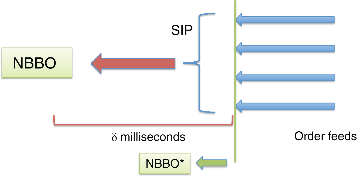
We illustrate this process and the potential for latency arbitrage in Fig. 1. Given order information from exchanges, the SIP takes some finite time, say δ milliseconds, to compute and disseminate the NBBO. A computationally advantaged trader who can process the order stream in less than δ milliseconds can simply out-compute the SIP to derive NBBO*, a projection of the future NBBO that will be seen by the public. By anticipating future NBBO, an HFT algorithm can capitalize on cross-market disparities before they are reflected in the public price quote, preemptively outbidding incoming orders when possible to pocket a small but sure profit. Naturally this precipitates an arms race, as an even faster trader can calculate an NBBO** to see the future of NBBO*, and so on.
Fig.1
Exploitation of latency differential. Rapid processing of the order stream enables private computation of the NBBO before it is reflected in the public quote from the SIP.
The latency arms race as sketched above is fundamentally an outgrowth of continuous trading: a property of mechanisms that distinguish precedence according to arbitrarily small time differences. By moving to a discrete-time model—which introduces short but finite clearing intervals (as in a frequent call market, or frequent batch auction)—we can neutralize small disparities in information access and response time. A driving question of this work is how such a mechanism-design intervention would affect market performance.
More broadly, we seek to understand not only the effects of latency arbitrage on market efficiency and liquidity, but also the interplay between fragmentation, clearing mechanisms, and latency arbitrage strategies in producing this performance. Such questions about HFT implications are inherently computational, as the very speed of operation renders details of internal market operations—especially the structure of communication channels—systematically relevant to market performance. In particular, the latencies between market events (transactions, price updates, order submissions) and when market participants observe these activities become pivotal, as even the smallest latency differential can significantly affect tradingoutcomes.
Previous work on the effects of high-frequency trading and market structure has relied primarily on either analytical models or examination of historical order and transaction data. Historical market data alone is insufficient as it cannot be used to answer counterfactual questions about the impact of modifying strategies or market rules. Analytical models, on the other hand, can capture essential aspects of market structure, but would require stifling complexity to specify the interactions between multiple entities or the precise timing of event occurrences (such as the propagation of information between markets and participants)—at which point a closed-form solution or any other reasoning would be rendered infeasible or otherwise unhelpful. Lacking suitable data to study these questions empirically2 we pursue a simulation approach.
We present a simple model that captures the effect of latency across two markets with a single security. Our model captures the interplay of latency and fragmentation as well as the regulatory environment responsible for current equity market structure, and we quantify the effect of latency arbitrage on surplus allocation as a function of latency and market rules. Using an agent-based approach, we implement our two-market model in a discrete-event simulation system that explicitly models the communication patterns between background investors, exchanges, and the SIP operating in current U.S. equity markets. We simulate the interactions between high-frequency and background traders, and we employ empirical game-theoretic analysis to identify equilibria under different market conditions.
We are primarily interested in the impact on efficiency of three different market features: presence of latency arbitrage, market fragmentation, and switching to discrete-time market clearing. Therefore, we compare allocative efficiency in equilibrium in our two-market model with equilibrium welfare in other models of market structure, including a consolidated continuous double auction market and a frequent call market. Our main finding is that in most of the model settings studied, latency arbitrage not only reduces profits of the background investors, but also diminishes surplus overall—even when the profits of LA are counted. Perhaps surprisingly, market fragmentation per se does not harm efficiency; in fact some degree of fragmentation mitigates the inefficient trades that are often executed by a continuous mechanism. The discrete-time frequent call market eliminates latency arbitrage by construction and, by virtue of temporal aggregation, yet more effectively matches orders, producing significantly greater surplus.
This study extends and supersedes our previous work (Wah and Wellman 2013). In that study, traders employed a fixed strategy for all market configurations and latency settings. The analysis presented here employs empirical game-theoretic methods to perform strategy selection for traders. The qualitative conclusions presented in the original study still hold; the results we report here serve to confirm those main points in a more extensive and strategically robust evaluation.
This paper is structured as follows. In Section 2, we discuss related work on agent-based financial markets and models of HFT and market structure. We present the general framework for our agent-based financial market models in Section 3. We describe our two-market model in Section 4, the computational approach we employ in Section 5, and our experimental setup in Section 6. In Section 7 we present our results, and we conclude in Section 8.
2Related work
2.1Agent-based financial markets
There is a substantial literature on agent-based modeling (ABM) of financial markets (Buchanan, 2009; Chen et al., 2012; Farmer and Foley, 2009; LeBaron, 2006), much of it geared to reproduce and thereby explain stylized facts from empirical studies of market behavior. For example, simulated markets have been constructed to reproduce phenomena observed in real stock markets, such as bubbles and crashes (LeBaron et al., 1999; Lee et al., 2011). Because agent behavior is shaped by the market environment, which includes interactions with other agents over time, such models can support causal reasoning (as in the study by (Thurner et al. (2012) establishing the effect of leverage on price volatility). One prominent example of an agent-based financial market is the Santa Fe artificial stock market (Palmer et al., 1994; LeBaron, 2004). ABM has also been used to model financial markets for applications such as portfolio selection (Jacobs et al., 2004) and determining the distributions of order and trading waiting times in a limit order book (Raberto and Cincotti, 2005).
2.2High-frequency trading models
Much of the current literature on the effects of HFT relies on the evaluation of historical order data. Hasbrouck and Saar (2013) use Nasdaq order data to construct sequences of linked messages describing trading strategies. They find that this low-latency activity improves short-term volatility, spreads, and market depth. Brogaard (2010) analyzes a 120-stock Nasdaq dataset that distinguishes HFT from non-HFT activity in order to assess the impact of high-frequency trading on liquidity, price discovery, and volatility. Prior work suggests that algorithmic trading improves liquidity (Hendershott et al., 2011); Angel et al. (2011) reach similar conclusions, finding that the emergence of automated trading and HFT has improved various market measures such as execution speed and spreads. Additional work suggests a link between HFT and increased volatility (Arnuk and Saluzzi, 2012). Foucault et al. (2015) examine latency arbitrage opportunities in currency markets, and provide evidence of a tradeoff between pricing efficiency and liquidity. In another study, Baron et al. (2012) find that some kinds of HFT activities directly harm ordinary investors.
Others rely on theoretical analysis to determine the optimal behavior of high-frequency traders. Avellaneda and Stoikov (2008) derive an optimal limit order submission strategy for a single high-frequency trader acting as a liquidity provider, running numerical simulations to assess the agent’s performance under varying strategies. Cohen and Szpruch (2012) propose a single-market model of latency arbitrage with one limit order book and two investors operating at different speeds. The fast trader employs a strategy that determines in advance the quantity the slow investor intends to trade, using this information to generate a risk-free profit. Jarrow and Protter (2012) develop a model of traders with differentials in speed and access to information, showing that HFT transactions can degrade price discovery, exacerbate volatility and increase mispricings—which HF arbitrageurs can then exploit.
In a rare application of ABM to HFT, Hanson (2012) finds that market liquidity and total surplus vary directly with the number of HF traders.
2.3Modeling market structure and clearing rules
Several prior works seek to identify the effects of market fragmentation and clearing rules, mainly via anecdotal evidence elicited from historical data. On the theoretical side, Mendelson (1987) investigates the effect of consolidation versus fragmentation of periodic call markets, without consideration of arbitrage between the submarkets. O’Hara and Ye (2011) use historical quote data and execution metrics to demonstrate that market fragmentation does not appear to harm measures such as spreads, execution speed, and efficiency. Bennett and Wei (2006) compare the execution costs of stocks that have switched from Nasdaq to the more consolidated NYSE, finding evidence that execution costs decline with order flow consolidation. Amihud et al. (2003) examine the response of equities on the Tel Aviv Stock Exchange to the exercise of corporate warrants, concluding that consolidation improves liquidity.
However, few prior studies attempt to directly model the communication latencies arising from market fragmentation and the resultant arbitrage opportunities, with the exception of Ding et al. (2014), who analyze NBBO latencies and the ability of HFTs to generate a synthetic NBBO. They conclude that price dislocations between the official and synthetic NBBOs can be exploited by HFTs for profit.
Switching to a discrete-time clearing mechanism, as in a frequent call market, has already been proposed as a means to eliminate the exploitation of latency differentials across multiple exchanges Wellman, 2009; Schwartz and Peng, 2013; Sparrow, 2012). Budish et al. (2013) analyze a theoretical model of a continuous limit order book, showing that HFT profits in equilibrium come from investors via wider spreads and that frequent batch auctions reduce the value of very small speed advantages. Others have proposed variants on the frequent call market with randomized clearing intervals (Sellberg, 2010; Industry Super Network, 2013), or randomized batching in conjunction with pro rata trade allocation rules, which may promote more equitable allocation of trades among investors (Farmer and Skouras, 2012; McPartland, 2013).
A number of other studies have focused not on the role of call markets in mitigating the harmful effects of HFT, but on the differences in market quality offered in a discrete-time versus a continuous market (Pancs, 2013; Pellizzari and Dal Forno, 2007) or an alternative market rule such as selective delay, in which cancellation orders are processed immediately but all other order types have a small delay (Baldauf and Mollner, 2014).
Empirical work on the effects of switching to periodic clearing is limited and again relies largely on the analysis of historical events (Webb et al., 2007; Kalay et al. 2002). For example, Amihud et al. (1997) find that switching from a daily call auction to a combination of discrete and continuous trading in the Tel Aviv Stock Exchange is associated with improvements in liquidity.
3Agent-based financial market models
In this section, we present our general framework for constructing computational agent-based financial market models. We focus on two types of markets in this study. The continuous double auction (CDA), in which orders are matched as they arrive, is used in virtually all stock markets today. This is in contrast to a periodic or frequent call market, in which orders are matched to trade at regular, fixed intervals (on the order of tenths of a second). We describe these two types of markets in Section 3.1.
Our market models are populated by background traders, who represent investors in the market. This is in contrast to market participants who exclusively pursue trading profit. We describe the valuation model of background traders in Section 3.2, and the class of background-trader strategies in Section 3.3.
3.1Market clearing mechanisms
The continuous double auction is a simple and standard two-sided market that forms the basis for most financial and commodities markets (Friedman, 1993). Agents submit bids, or limit orders, specifying the maximum price at which they would be willing to buy a unit of the security, or the minimum price at which they would be willing to sell (hence, the CDA is often referred to as a limit order market in the finance literature). CDAs are continuous in the sense that when a new order matches an existing incumbent order in the order book, the market clears immediately and the trade is executed at the price of the incumbent order—which is then removed from the book. Orders may be submitted at any time, and a buy order matches and transacts with a sell order when the limits of both parties can be mutuallysatisfied.
An alternative to continuous trading is a frequent call market or frequent batch auction, in which order matching is performed only at discrete, periodic intervals (e.g., on the order of tenths of a second). A discrete-time market facilitates more efficient trading by aggregating supply and demand and matching orders to trade at a uniform price (Biais et al. 2005; Gode and Sunder, 1997; Wah and Wellman, 2013). As in the CDA, traders in the frequent call market can arrive and submit orders at any time. The submitted limit orders remain in the order book until executed or canceled. In a frequent call market, orders are accumulated over a series of fixed-length clearing intervals. Orders are processed in batch via a uniform-price auction: at the end of each interval, the market computes the aggregate supply and demand functions based on current outstanding orders. No trade occurs if supply and demand do not intersect. If supply and demand intersect, the market clears at a uniform price that best matches the aggregated buy and sell orders, i.e., where supply equals demand. Buy orders strictly greater than the computed price, as well as sell orders strictly less than this price, will execute and subsequently be removed from the order book. If supply and demand intersect horizontally or at a single point, there exists a unique clearing price for the given interval. Orders that do not trade in the current period remain outstanding and carry over to the next clearing interval.
A frequent call market effectively eliminates the latency advantages of HFTs by hiding all submitted orders within each clearing interval, as in a sealed-bid auction. The removal of time priority within each batch period helps ensure that standing offers cannot be readily picked off by incoming orders, thereby transforming the competition on speed into a competition on price. This ensures that there is no significant advantage to receiving and responding to information faster than other traders, because all orders within a clearing interval are processed and matched at the same time. Periodic clears every second or so would be imperceptible to most investors but would prevent the exploitation of small speed advantages, thus curbing HFT participation in the latency armsrace.
In our implementation of these market models, prices are fine-grained but discrete, taking values at integer time points. Agents arrive at designated times, and submit limit orders to their associated market(s). Each market continually publishes a price quote consisting of two parts, the BID and the ASK. Other bids in the order book are not visible to traders. CDA price quotes reflect the best current outstanding orders, whereas call market quotes reflect the best outstanding orders immediately following the latest market clear. Specifically, for the CDA, BIDt is the price of the highest buy offer at time t and ASKt is the price of the lowest offer to sell. For the frequent call market, BIDt corresponds to the highest outstanding buy offer as of the most recent clear time tc, so that BIDt = BIDt′ for any tc ≤ t′ ≤ t. Similarly, ASKt is the lowest outstanding offer to sell as of tc. The difference between the two quote components is called the BID-ASK spread. An invariant for both the CDA and the call market is that BID < ASK. Otherwise, the orders would have matched and been removed from the order book—either immediately in the case of the CDA or upon the clear in the frequent call market.
3.2Valuation model
Each background trader has a valuation for the security in question, comprised of private and common components. The common component is defined as follows. We denote by rt the common fundamental value for the security at time t. The fundamental time series is generated by a mean-reverting stochastic process:
Parameter κ ∈ [0, 1] specifies the degree to which the fundamental reverts back to the mean
The private component for agent i is a vector Θi representing differences in the agent’s private benefits of trading given its net position, similar to the model of Goettler et al. (2009). This private valuation vector reflects individual preferences in the marginal value of the security (e.g., due to risk aversion, outside portfolio holdings of related securities, or immediate liquidity needs), as well as preferences regarding urgency to trade. The vector is of size 2qmax, where qmax is the maximum number of units the agent can be long or short at any time, with
Element
We generate Θi from a set of 2qmax values drawn independently from a Gaussian distribution. Let
Background trader i’s valuation v for the security at time t is based on its current position qt and the value of the global fundamental at time T, the end of the trading horizon:
For a single-quantity limit order transacting at time t and price p, a trader obtains surplus:
Since the price and fundamental terms cancel out in exchange, the total surplus achieved when agent B buys from agent S is
3.3Background-trader strategies
There is an extensive literature on autonomous bidding strategies for CDAs (Das et al., 2001; Friedman, 1993; Wellman, 2011). In this study, we consider trading strategies in the so-called Zero Intelligence (ZI) family (Gode and Sunder, 1993).
The background traders arrive at the market according to a Poisson process with rate λBG. On each arrival, the trader first withdraws its previous order (if not transacted yet). It is then assigned to buy or sell (with equal probability), and accordingly submits an order to buy or sell a single unit. (Traders are randomly reassigned to buy or to sell each time they arrive.) Background traders are notified of all transactions and current price quotes with zero delay, and may use this information in computing their bids. Agents may trade any number of times, as long as their net positions do not exceed qmax (either long or short).
Recall that each background trader has an individual valuation for the security comprised of private and common components, as described in the previous section. Based on this valuation, each background trader obtains a payoff at the end of the simulation period. This payoff is computed as the sum of the private value of the trader’s holdings, the net cash flow from trading, and the liquidation proceeds of any accumulated inventory at the end-time fundamental value rT (i.e., the common component of the valuation).
A ZI trader assesses its valuation vi (t) at the time of market entry t, using an estimate
The ZI agent then submits a bid shaded from this estimate by a random offset—the degree of surplus it demands from the trade. The amount of shading is drawn uniformly from range [Rmin, Rmax]. Specifically, a ZI trader i arriving at time t with current position q submits a limit order for a single unit of the security at price
We extend ZI by including a threshold parameter η ∈ [0, 1], whereby if the agent could achieve a fraction η of its requested surplus at the current price quote, it would simply take that quote rather than posting a limit order to the book. Setting η = 1 is equivalent to the strategy without employing the threshold.
4Two-market model
We present a simple model for latency arbitrage across two markets populated by a single high-frequency trader and multiple background traders. We describe the specifics of this model in Section 4.1. The valuation model and class of strategies employed by the background investors are as described in Sections 3.2 and 3.3, respectively. In Section 4.2, we discuss the behavior of the latency arbitrageur. We present an example of how a latency arbitrage opportunity can arise in this two-market model in Section 4.3.
4.1Model description
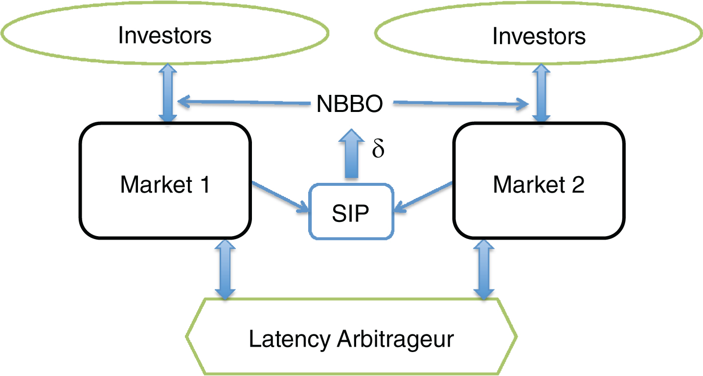
Our model of latency arbitrage consists of one security traded on two markets, each employing a continuous double auction mechanism (Section 3.1). The two markets are linked by a public NBBO signal (see Fig. 2). Limit orders lodged in either market are forwarded to the SIP, which calculates and reports an NBBO—based on the quotes from the two markets—with some finite delay δ. This latency reflects the time required to receive information about activities in the two markets and compute an updated public price signal.
Fig.2
Two-market model with one infinitely fast latency arbitrageur and multiple background investors. A single security is traded on the two markets. Each background investor is associated primarily with one of the two markets, and its order is routed to its alternate market if and only if the NBBO quote indicates an immediate execution. The latency arbitrageur has undelayed access to both markets, so it can immediately detect arbitrage opportunities arising from the delay in NBBO calculation.
Retail and institutional investors generate limit orders according to an evolving fundamental (driven by news) and other private factors. Each non-HF investor is primarily associated with one of the two markets. An order is sent to the trader’s primary market unless the NBBO indicates that it could be executed in the alternate market at a price better than that available on the primary market.
More precisely, let BIDj and ASKj, where j ∈ {1, 2}, denote the current BID and ASK quotes, respectively, in market j. Similarly, let BIDN and ASKN represent the NBBO quote. Background traders have direct access to the quotes on their primary market and the NBBO, but not to those on the alternate market. Suppose a trader associated with market 1 generates a limit order to buy a unit at price p. This order is routed to market 2 if and only if p ≥ ASKN and ASKN < ASK1. Otherwise, the order goes to market 1, the trader’s primary market. Note that the conditions for submitting to the alternate market entail that the trader’s order would execute there immediately, if in fact the NBBO reflects the current global state. If the order is routed to the primary market, it may execute right away (if p ≥ ASK1); otherwise, it is added to market 1’s order book. The rule for routing sell orders is analogous.
The latency arbitrageur in this model can determine the best prices in each market before the NBBO updates, due to its ability to receive and process order streams faster than background investors. It can thus directly detect an arbitrage situation, which occurs whenever BID1 > ASK2 or BID2 > ASK1. We assume the arbitrageur can respond infinitely fast, so it immediately takes the profit from such arbitrage situations by submitting executable orders to the two markets. Note that the arbitrage opportunity can arise only to the extent that the NBBO information is out of date. If the SIP were able to compute and publish the NBBO with zero latency, then a new order would always be routed correctly and would thereby execute immediately if there were a matching order in either market. Any finite delay, however, opens the possibility that an order is routed to the investor’s primary market, despite there being a matching order in the alternate market that had arrived too recently to be admitted in the available NBBO. An out-of-date NBBO can also cause an order to be improperly routed to the alternate market despite it no longer matching there, even if there is a matching order in the primary market.
4.2Latency arbitrageur
The latency arbitrageur (LA) in the two-market model operates as follows. LA first obtains current price quotes in both markets, then checks whether an arbitrage situation exists. We denote the best price available to sell at by
4.3Example
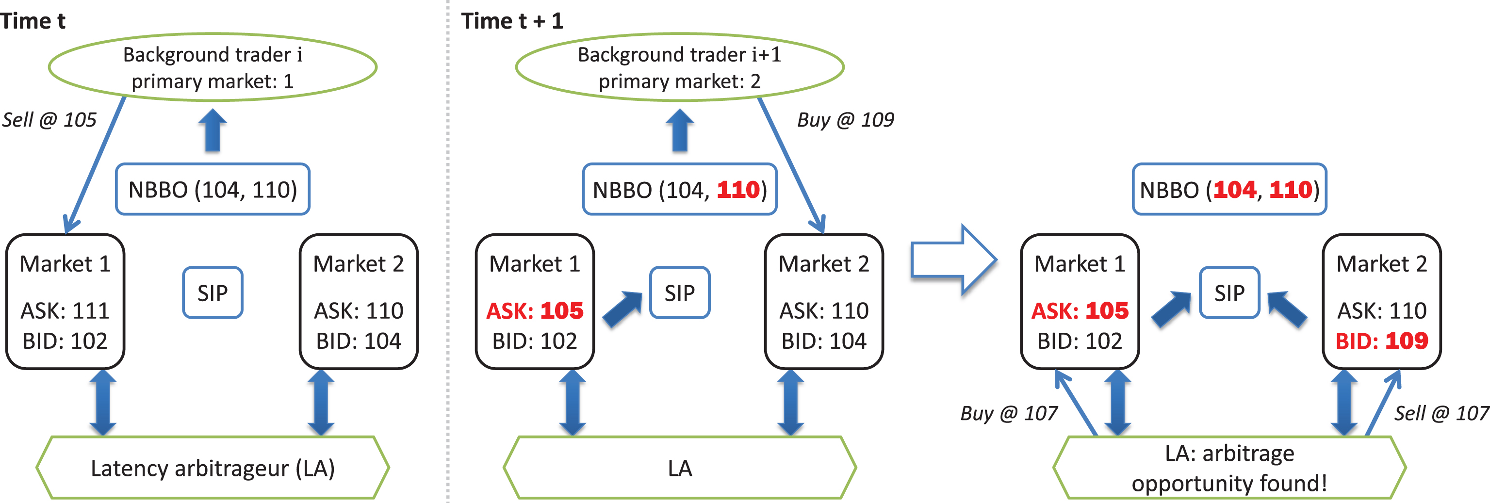
Figure 3 illustrates how a latency arbitrage opportunity may arise in our two-market model. At time t, the NBBO quote is BIDN = 104 and ASKN = 110. Consider background trader i, who wishes to submit a sell order at 105 to market 1, its primary market. To determine the order routing, BID1 is compared with the NBBO. As BIDN > BID1, the alternate market appears to be superior. However, a sell offer at 105 would not transact immediately (since BIDN = 104), so agent i’s order is routed to market 1. At the beginning of time t + 1, for latency δ > 1, the SIP has not yet updated the NBBO to include the order submitted at time t. Thus, the NBBO available to background investors is out of date: the correct quote would be (104, 105), but the NBBO at time t + 1 is still (104, 110) and matches ASK2 in market 2, incoming agent i + 1’s primary market. Consequently, agent i + 1’s buy order at price 109 is routed to its primary market. At this point, BID2 (at price 109, submitted by agent i + 1) exceeds ASK1 (at price 105, submitted by agent i), which defines an arbitrage opportunity. Since LA is infinitely fast, it capitalizes on this disparity by submitting bids to buy at 107 in market 1 and sell at 107 in market 2, realizing a profit of 4.
Fig.3
Emergence of a latency arbitrage opportunity over two time steps in the two-market model. All orders are for single-unit quantities. A red, bolded price highlights a discrepancy between the actual market state and the NBBO, represented in the diagram as (BIDN, ASKN). At time t, the NBBO is up to date. Background trader i wishes to sell at price 105. Since BIDN < 105 (which indicates non-immediate execution), the investor’s order is routed to market 1. At time t + 1, the NBBO is out of date, as the SIP updates the public quote with some delay δ. Background trader i + 1 wishes to buy at 109; based on the NBBO, its order is routed to market 2, its primary market. (Had its order been routed to market 1, its bid would have transacted immediately.) The submission of its order to the inferior market opens up an arbitrage opportunity between the two markets (BID2 > ASK1), which LA immediately exploits for a guaranteed profit.
5Computational approach
To answer questions regarding the interplay between trader behavior and market structure, we employ a computational approach that combines agent-based modeling (ABM), simulation, and equilibrium computation. In ABM, autonomous agents interact dynamically based on algorithmic rules. These rules govern each agent’s actions and responses, but do not explicitly define or specify aggregate outcomes; instead, system-level phenomena are a consequence of collective agent behavior. We simulate interactions between agents in a variety of market environments to study the effect of market structure and trader strategies on market performance. We present our simulation system in Section 5.1.
Using trader performance assessed from simulation runs, we employ game-theoretic analysis to evaluate traders’ strategic interactions with each other under a variety of market settings. We focus on trader behavior in equilibrium, when all market participants are best responding to each others’ strategies in order to optimize their own gains from trade. Equilibrium outcomes offer a basis for predicting agents’ actions taking account of their strategic decision making. We explore various market scenarios and environments in order to characterize trader behavior in equilibrium under different market conditions. We describe the methodology we employ to identify equilibria in Section 5.2.
In order to mitigate the stochasticity in our simulations and reduce sampling error, we collect large numbers of observations for each environment setting and trader population of interest. We utilize the EGTAOnline infrastructure (Cassell and Wellman, 2013) to conduct and manage our experiments, and we run our simulations on the high-performance computing cluster at the University of Michigan.
5.1Discrete-event simulation
The financial markets we study are stochastic, dynamic systems with discrete states that change in response to communication events. These events occur at high frequency, even on the order of microseconds. To faithfully model such systems in simulation, ensuring the unambiguous timing of agent and market interactions is paramount. This necessitates fine-grained modeling at the level of communication. We therefore design our system based on principles of discrete-event simulation (DES), which affords the precise specification of temporal changes in system state. In the DES framework, a simulation run is modeled as a sequence of events (Banks et al., 2005). Each event is an instantaneous occurrence that marks a change to the system state at a given time, and events are maintained in a queue ordered by time of occurrence.
Our financial market simulation system, based on that described in detail by Wah and Wellman (2013), affords sufficient versatility to model a wide range of market environments, including variform populations of market participants, as well as different market structures (e.g., varying in the number of markets or types of market mechanisms employed). The simulator has been extended by other members of the Strategic Reasoning Group at the University of Michigan and employed in several other studies.
5.2Empirical game-theoretic analysis
We model the strategic situation of background traders as a normal-form game, where each player (trader) has a set of available strategies, and the outcome is a function of the joint choice of strategies (the strategy profile) and stochastic events in the market environment. Players may select from the strategy set deterministically (adopting a pure strategy) or according to a probability distribution (a mixed strategy). The support of a strategy is the set of pure strategies played with nonzero probability (hence, a pure strategy has singleton support). The game model maps strategy profiles to vectors of payoffs, representing the utility each player obtains in expectation over the profile outcomes.
The simulation system discussed in the previous section takes as input a strategy profile and generates as output a sample outcome. Through a process of empirical-game theoretic analysis (EGTA) (Wellman, 2006) we systematically generate samples in this way to estimate a model of the overall game. Given the estimated game model, we can apply standard solution concepts to characterize or predict agent behavior. We focus here on Nash equilibrium (NE), in which each player selects a strategy maximizing its expected payoff, given the strategies of the other players.
In this study, we model the market as a symmetric game, which means that each player has the same available strategy set, and each has the same payoff as a function of its own strategy and the set of other-agent strategy choices. In other words, payoffs depend only on the number of agents playing each strategy, not on the identities of the agents playing them. We also focus attention on symmetric NE, in which each player selects the same (possibly mixed) strategy in equilibrium. Note that even for a symmetric profile, on any given run the players will generally choose different strategies (a consequence of independent selection from the mixture), and will also generally have heterogeneous private valuations.
5.3EGTA process
To analyze a game, we apply EGTA in an iterative manner, interleaving exploration of the profile space with analysis of the empirical game model induced by average payoffs in simulation. We start by simulating all the symmetric pure-strategy profiles, where a single strategy is shared by all players. Exploration then spreads through their neighbors, that is, those profiles related by single-agent deviations.
Observed payoffs from simulation runs of a given profile are added incrementally to the empirical game’s payoff matrix. For this reason, the game is incomplete at any point during the EGTA process, as some profiles have been empirically evaluated whereas others have not. Each update to the empirical game’s payoff matrix generates an intermediate game model. As payoffs from simulation are incorporated into the empirical game, we analyze each successive intermediate game model by computing (mixed) equilibria for each complete subgame. A (normal-form) subgame is the game obtained by restricting the set of strategies, and a complete subgame is defined as a subgame for which all profiles have been evaluated by simulation. The symmetric Nash equilibria of the complete subgames are candidates for equilibria in the full game. If we can identify a strategy in the full strategy set that beneficially deviates from the candidate, we say the candidate is refuted. A candidate profile is confirmed as an NE when all possible deviations have been evaluated, and none are beneficial. We confirm or refute each candidate by evaluating deviations to strategies outside their subgames. If a candidate is refuted, we construct a new subgame by adding the best response to its support, and proceed to explore the corresponding subgame.
We simulate additional profiles for a game until we have confirmed at least one symmetric NE, evaluated every pure-strategy symmetric profile, and pursued with some degree of diligence every equilibrium candidate encountered. More specifically, we continue to refine the empirical game with additional simulations until the following conditions are met:
1 at least one equilibrium is confirmed,
2 all non-confirmed candidates are refuted (up to a threshold support size), and
3 for all refuted candidates (up to the threshold support size), we have explored subgames formed by adding the best response to the candidate’s support.
The procedure described above seeks to either confirm or refute the equilibrium candidates detected in our exploration of the strategy space. As we are not able to exhaustively search the entire profile space, however, additional qualitatively distinct equilibria are always possible. In addition, the equilibria we find are subject to refutation by other strategies outside the specified set. Our search process described above attempts to evaluate all promising equilibrium candidates (e.g., by exploring subgames extending the support of a refuted candidate with the best response), but identifying these is not guaranteed.
5.4Game reduction
Even with a moderate number of players, the game size (number of possible strategy profiles) grows exponentially with the number of players and strategies, rendering analysis of the full game computationally infeasible. As such, we apply aggregation to approximate the many-player games as games with fewer players: We employ the technique of deviation-preserving reduction (DPR) developed by Wiedenbeck and Wellman (2012) to construct a reduced-game approximation of the full game.
DPR preserves the payoffs from single-player, unilateral deviations, and maintains in the reduced game the same proportion of opponents playing each strategy as in the full game. In a deviation-preserving reduced game, each player views itself as controlling one full-game agent and views the other-agent profile in the reduced game as an aggregation of all other players in the full game. Although the equilibrium approximations obtained via DPR are not guaranteed estimates, DPR has been shown to produce good approximations in other games (Wiedenbeck and Wellman, 2012).
DPR defines reduced-game payoffs in terms of payoffs in the full game as follows. Consider first an N-player symmetric game, reduced to a k-player game, for k < N. The payoff for playing strategy s1 in the reduced game, with other agents playing strategies (s2, dotsc, sk), is given by the payoff of playing s1 in the full N-player game when the other N - 1 agents are evenly divided (
6Experiments
To isolate the ramifications of market fragmentation, we consider two consolidated market configurations in addition to the two-market model: a CDA and a frequent call market. Recall that in contrast to a continuous-time market, clearing in a frequent call market takes place at designated intervals (Section 3.1). A frequent call market eliminates latency arbitrage opportunities, as the periodic clearing mechanism makes it impossible to gain or exploit informational advantages over other market participants within the clearing interval.
In exploring the relationship between trader behavior and market structure, we are interested in the following performance characteristics:
Allocative efficiency. Total surplus (welfare) is our key measure of market performance. Welfare indicates how well the market allocates trades according to underlying private valuations.
Liquidity. Markets are liquid to the extent they maintain availability of opportunities to trade at prevailing prices. Two liquidity-related metrics are fast execution and tight BID-ASK spreads. We measure execution time by the interval between order submission and transaction for orders that eventually trade. Execution time is potentially important to investors for many reasons, including the risk of changes in valuation while an order is pending, the effect of transaction delay on other contingent decisions, and general time preference. We also measure spread, which is the distance between prices quoted to buyers and sellers (Section 3.1).
Our experiments (Table 1) evaluate a number of market features, defined by different combinations of market configurations:
1 Presence of latency arbitrage: Two-market configurations with or without LA.
2 Market fragmentation: Two-market configurations versus continuous one-market (consolidated) configuration.
3 Market clearing rules: One-market configurations with continuous (CDA) or discrete-time (call) clearing. To facilitate direct comparison, in each run we set the clearing interval of the call market to equal the NBBO update latency.
Table 1
Experimental design for evaluating different market features
| Features | Market configurations | |||
| 2M (LA) | 2M (no LA) | CDA | Call | |
| Latency arbitrage | + | + | ||
| Market fragmentation | + | + | + | |
| Discrete-time clearing | + | + | ||
Each row of the table describes the market configurations included (as indicated by the plus symbol) in evaluating a given market feature. The four market configurations are the two-market model (2M) both with and without LA, the consolidated CDA, and the frequent call market.
6.1Environment settings
We evaluate and compare the performance of the four market structure configurations (two-market model with and without LA, CDA, and frequent call market) within three distinct environments. For the fragmented cases, an equal proportion of background traders is assigned primary affiliation with each market in a model. In the consolidated call market, orders transact at a uniform price each time the market clears; this price is computed to best match supply and demand (Section 3.1).
In defining our environments, we selected environment parameters that generate sufficient arbitrage opportunities and also replicate the original findings for fixed-strategy, non-equilibrium comparisons from our previous study (Wah and Wellman, 2013). To do so, we explored a number of environments, varying the number of traders, trading horizon length, degree of mean reversion, and variance in both the fundamental and private values. In these runs, all traders employed a fixed strategy with η = 1, similar to the agents in our previous study. We selected the environments reproducing the qualitative effects previously observed as the starting point for the extended strategic analysis of the current study.
The threshold α for LA is fixed at a small value such that any possible price difference is sufficient for the arbitrageur to exploit. We set qmax = 10, mean fundamental value
Table 2
ZI strategy combinations included in empiricalgame-theoretic analysis
| Rmin | Rmax | η |
| 0 | 125 | 1 |
| 0 | 250 | 1 |
| 0 | 500 | 1 |
| 250 | 500 | 1 |
| 0 | 1000 | 1 |
| 500 | 1000 | 0.4 |
| 500 | 1000 | 1 |
| 0 | 1500 | 0.6 |
| 1000 | 2000 | 0.4 |
| 0 | 2500 | 0.4 |
| 0 | 2500 | 1 |
The environments differ in number of background traders (N), background-trader (re)entry rate (λBG), value of the mean-reversion parameter (κ), and time horizon (T). For each market configuration in an environment, we explore a range of latency settings, with a minimum difference (or order of magnitude) of Δδ ∈ {10, 100}. The configurations of parameter settings are listed in Table 3. The arrival rate parameter is either λBG = 0.05 or λBG = 0.005; each ZI agent arrives, on average, every 20 or 200 time steps.
Table 3
Parameter settings for the three market environments
| Environment | N | λBG | κ | T | Δδ |
| 1 | 24 | 0.05 | 0.05 | 15000 | 100 |
| 2 | 238 | 0.0005 | 0.02 | 10000 | 10 |
| 3 | 58 | 0.0005 | 0.02 | 5000 | 10 |
6.2Empirical games
We examine 23 empirical games within environment 1, which cover the four market configurations across 8 settings of latency δ ∈ {0, 100, 200, 300, 400, 600, 700, 900}. For environment 2 we include 8 empirical games (δ ∈ {0, 50, 100}), and examine 14 games within environment 3 (δ ∈ {0, 25, 50, 75, 100}). Table 4 lists all 45 empirical games across the three market environments. The games in a given environment include one single-market CDA game (which is independent of latency), and one game for each of the other three market configurations (two fragmented cases and one with periodic clears) per latency setting simulated. At latency 0, the frequent call market is equivalent to the CDA, and the two models with fragmentation are equivalent as there are no arbitrage opportunities at zero latency.
Table 4
Empirical games across the three market environments
| Environment 1 | Environment 2 | Environment 3 | |||
| Configuration | Latency | Configuration | Latency | Configuration | Latency |
| CDA | – | CDA | – | CDA | – |
| 2M | 0 | 2M | 0 | 2M | 0 |
| 2M (no LA), 2M (LA), Call | 100 | 2M (no LA), 2M (LA), Call | 50 | 2M (no LA), 2M (LA), Call | 25 |
| 2M (no LA), 2M (LA), Call | 200 | 2M (no LA), 2M (LA), Call | 100 | 2M (no LA), 2M (LA), Call | 50 |
| 2M (no LA), 2M (LA), Call | 300 | 2M (no LA), 2M (LA), Call | 75 | ||
| 2M (no LA), 2M (LA), Call | 400 | 2M (no LA), 2M (LA), Call | 100 | ||
| 2M (no LA), 2M (LA), Call | 600 | ||||
| 2M (no LA), 2M (LA), Call | 700 | ||||
| 2M (no LA), 2M (LA), Call | 900 | ||||
The empirical games for each environment include a consolidated CDA, which is independent of latency, and one game at each latency setting for the other three market configurations. At latency 0, the fragmented models are equivalent to the CDA, as there are no arbitrage opportunities. Latency here with regards to the frequent call market indicates the length of the clearing interval.
We compare the equilibria found in the empirical games according to the experimental design described in Table 1 to evaluate the effect of latency arbitrage, market fragmentation, and batching on market efficiency and liquidity.
The strategic situations for each market structure are modeled as symmetric games (Section 5.2). We apply deviation-preserving reduction (Section 5.4) to generate an approximation of the full game with fewer players. Specifically, we estimate 4-player reduced games from full games with N ∈ {24, 238, 58}3 players.
7Results
We find in these settings that the presence of a latency arbitrageur reduces total surplus (Section 7.1) and has a mixed effect on market liquidity (Section 7.3). Eliminating fragmentation can improve surplus (Section 7.2) and execution metrics (Section 7.3). Replacing continuous markets with frequent call markets eliminates latency arbitrage opportunities and achieves substantial efficiency gains in all three environments (Section 7.4). Our results are summarized in Table 5.
Table 5
Overview of experimental results
| Feature | Section | Effect on market efficiency | Effect on liquidity |
| Latency arbitrage | 7.1,7.3 | Generally degrades efficiency, but increased bid shading in low mean reversion environments alleviates inefficiencies caused by LA | LA exacerbates spreads, and execution times vary by environment based on bid shading in equilibrium |
| Market fragmentation | 7.2,7.3 | Can benefit continuous markets by admitting fewer inefficient trades (due to vagaries of the arrival sequence of orders), but LA defeats this benefit | Execution times vary by environment, with consolidation improving liquidity in the fragmented model without LA when traders do not shade more |
| Discrete-time clearing | 7.4 | Significantly improves surplus across all environments | Increases execution times but effect is fairly small in clock time if market clears occur frequently, such as every second |
We identified 1–3 equilibria for each of the 23 games in environment 1 (Tables 6 and 7), the 8 games in environment 2 (Tables 8 and 9), and the 14 games in environment 3 (Tables 10 and 11). For each equilibrium, we estimated background-trader surplus, as well as LA profit if applicable, by sampling 500 profiles according to the equilibrium mixture, and running 100 simulations per sampled profile (50,000 full-game simulations in total).
Table 6
Symmetric equilibria for environment 1, N = 24
| Model | Latency | Surplus | Profit | mid | η |
| CDA | – | 10114 | – | 1298 | 0.458 |
| CDA | – | 10383 | – | 1377 | 0.4 |
| 2M | 0 | 11807 | – | 1250 | 0.4 |
| 2M | 0 | 11393 | – | 1034 | 0.506 |
| Call | 100 | 13471 | – | 682 | 0.695 |
| 2M (no LA) | 100 | 9400 | – | 1439 | 0.4 |
| 2M (no LA) | 100 | 10373 | – | 1008 | 0.4 |
| 2M (LA) | 100 | 5919 | 3487 | 1266 | 0.4 |
| Call | 200 | 13308 | – | 687 | 0.703 |
| 2M (no LA) | 200 | 10621 | – | 1144 | 0.4 |
| 2M (LA) | 200 | 6358 | 3164 | 1420 | 0.4 |
| Call | 300 | 13107 | – | 721 | 0.679 |
| 2M (no LA) | 300 | 10386 | – | 1402 | 0.4 |
| 2M (no LA) | 300 | 11244 | – | 913 | 0.4 |
| 2M (LA) | 300 | 6398 | 3224 | 1414 | 0.4 |
| Call | 400 | 13004 | – | 383 | 1 |
| Call | 400 | 12771 | – | 640 | 0.747 |
| Call | 400 | 12686 | – | 460 | 0.961 |
| 2M (no LA) | 400 | 10438 | – | 1399 | 0.4 |
| 2M (LA) | 400 | 6130 | 4018 | 1080 | 0.4 |
| Call | 600 | 12932 | – | 321 | 1 |
| Call | 600 | 12403 | – | 704 | 0.76 |
| Call | 600 | 12526 | – | 675 | 0.701 |
| 2M (no LA) | 600 | 10182 | – | 750 | 0.4 |
| 2M (no LA) | 600 | 11128 | – | 845 | 0.4 |
| 2M (LA) | 600 | 7459 | 4349 | 1257 | 0.429 |
| 2M (LA) | 600 | 6457 | 4460 | 932 | 0.4 |
| 2M (LA) | 600 | 6509 | 3276 | 1411 | 0.429 |
| Call | 700 | 12910 | – | 294 | 0.957 |
| Call | 700 | 12868 | – | 287 | 0.958 |
| 2M (no LA) | 700 | 9138 | – | 1343 | 0.442 |
| 2M (no LA) | 700 | 11302 | – | 881 | 0.4 |
| 2M (LA) | 700 | 5256 | 2958 | 1453 | 0.4 |
| Call | 900 | 12613 | – | 251 | 1 |
| 2M (no LA) | 900 | 8641 | – | 1459 | 0.498 |
| 2M (no LA) | 900 | 12358 | – | 1250 | 0.4 |
| 2M (no LA) | 900 | 10710 | – | 1384 | 0.4 |
| 2M (LA) | 900 | 4807 | 3121 | 1403 | 0.426 |
| 2M (LA) | 900 | 6819 | 4825 | 1184 | 0.479 |
Symmetric equilibria for empirical games for environment 1, one per latency (or clearing interval) setting per market configuration, N = 24, calculated from the 4-player DPR approximation. The four market configurations are the two-market model (2M) both with and without LA, the consolidated CDA, and the frequent call market. Each row of the table describes one equilibrium found and its average values for background-trader surplus, LA profit, and two strategy parameters: mid (the midpoint of ZI range [Rmin, Rmax]) and threshold η. Values presented are the average over strategies in the profile, weighted by mixture probabilities. Surplus values are means from thousands of simulations of the full game, where strategies are randomly sampled from the equilibrium mixed-strategy profile.
Table 7
Complete specifications of symmetric equilibria for environment 1, N = 24
| Model | Latency | 125 | 250 | 500 | 500** | 1000 | 1000‡ | 1000** | 1500† | 2000‡ | 2500° | 2500 |
| CDA | – | 0 | 0 | 0 | 0.096 | 0 | 0 | 0 | 0 | 0.528 | 0.376 | 0 |
| CDA | – | 0 | 0 | 0 | 0 | 0 | 0 | 0 | 0 | 0.507 | 0.493 | 0 |
| 2M | 0 | 0 | 0 | 0 | 0 | 0 | 0 | 0 | 0 | 0 | 1 | 0 |
| 2M | 0 | 0 | 0 | 0 | 0.177 | 0 | 0.123 | 0 | 0 | 0 | 0.7 | 0 |
| Call | 100 | 0.15 | 0.324 | 0 | 0 | 0 | 0 | 0 | 0.052 | 0 | 0.474 | 0 |
| 2M (no LA) | 100 | 0 | 0 | 0 | 0 | 0 | 0 | 0 | 0 | 0.758 | 0.242 | 0 |
| 2M (no LA) | 100 | 0 | 0 | 0 | 0 | 0 | 0.602 | 0 | 0 | 0.239 | 0.159 | 0 |
| 2M (LA) | 100 | 0 | 0 | 0 | 0 | 0 | 0.237 | 0 | 0 | 0.537 | 0.226 | 0 |
| Call | 200 | 0.368 | 0 | 0.094 | 0 | 0.042 | 0 | 0 | 0 | 0 | 0.496 | 0 |
| 2M (no LA) | 200 | 0 | 0 | 0 | 0 | 0 | 0.381 | 0 | 0 | 0.338 | 0.281 | 0 |
| 2M (LA) | 200 | 0 | 0 | 0 | 0 | 0 | 0 | 0 | 0 | 0.679 | 0.321 | 0 |
| Call | 300 | 0.094 | 0.371 | 0 | 0 | 0 | 0 | 0 | 0 | 0 | 0.535 | 0 |
| 2M (no LA) | 300 | 0 | 0 | 0 | 0 | 0 | 0 | 0 | 0 | 0.608 | 0.392 | 0 |
| 2M (no LA) | 300 | 0 | 0 | 0 | 0 | 0 | 0.692 | 0 | 0 | 0.036 | 0.272 | 0 |
| 2M (LA) | 300 | 0 | 0 | 0 | 0 | 0 | 0 | 0 | 0 | 0.655 | 0.345 | 0 |
| Call | 400 | 0 | 0 | 0.835 | 0.036 | 0 | 0 | 0 | 0 | 0 | 0 | 0.129 |
| Call | 400 | 0 | 0.416 | 0 | 0.163 | 0 | 0 | 0 | 0 | 0 | 0.421 | 0 |
| Call | 400 | 0 | 0.055 | 0 | 0.347 | 0.501 | 0 | 0 | 0.097 | 0 | 0 | 0 |
| 2M (no LA) | 400 | 0 | 0 | 0 | 0 | 0 | 0 | 0 | 0 | 0.595 | 0.405 | 0 |
| 2M (LA) | 400 | 0 | 0 | 0 | 0 | 0 | 0.47 | 0 | 0 | 0.258 | 0.272 | 0 |
| Call | 600 | 0 | 0.477 | 0 | 0 | 0.523 | 0 | 0 | 0 | 0 | 0 | 0 |
| Call | 600 | 0.22 | 0 | 0 | 0 | 0.379 | 0 | 0 | 0 | 0 | 0.401 | 0 |
| Call | 600 | 0.271 | 0.207 | 0 | 0.023 | 0 | 0 | 0 | 0 | 0 | 0.499 | 0 |
| 2M (no LA) | 600 | 0 | 0 | 0 | 0 | 0 | 1 | 0 | 0 | 0 | 0 | 0 |
| 2M (no LA) | 600 | 0 | 0 | 0 | 0 | 0 | 0.81 | 0 | 0 | 0 | 0.19 | 0 |
| 2M (LA) | 600 | 0 | 0 | 0 | 0 | 0 | 0 | 0.029 | 0 | 0 | 0.971 | 0 |
| 2M (LA) | 600 | 0 | 0 | 0 | 0 | 0 | 0.635 | 0 | 0 | 0 | 0.365 | 0 |
| 2M (LA) | 600 | 0 | 0 | 0 | 0 | 0 | 0 | 0 | 0 | 0.643 | 0.308 | 0.049 |
| Call | 700 | 0.162 | 0.484 | 0.022 | 0 | 0.258 | 0 | 0 | 0.008 | 0 | 0.066 | 0 |
| Call | 700 | 0.185 | 0.471 | 0 | 0.059 | 0.216 | 0 | 0 | 0 | 0 | 0.069 | 0 |
| 2M (no LA) | 700 | 0 | 0 | 0 | 0 | 0 | 0 | 0 | 0.209 | 0.791 | 0 | 0 |
| 2M (no LA) | 700 | 0 | 0 | 0 | 0 | 0 | 0.739 | 0 | 0 | 0 | 0.261 | 0 |
| 2M (LA) | 700 | 0 | 0 | 0 | 0 | 0 | 0.006 | 0 | 0 | 0.826 | 0.168 | 0 |
| Call | 900 | 0 | 0.246 | 0.498 | 0.256 | 0 | 0 | 0 | 0 | 0 | 0 | 0 |
| 2M (no LA) | 900 | 0 | 0 | 0 | 0 | 0 | 0 | 0 | 0 | 0.836 | 0 | 0.164 |
| 2M (no LA) | 900 | 0 | 0 | 0 | 0 | 0 | 0 | 0 | 0 | 0 | 1 | 0 |
| 2M (no LA) | 900 | 0 | 0 | 0 | 0 | 0 | 0 | 0 | 0 | 0.537 | 0.463 | 0 |
| 2M (LA) | 900 | 0 | 0 | 0 | 0 | 0 | 0 | 0.129 | 0.871 | 0 | 0 | 0 |
| 2M (LA) | 900 | 0 | 0 | 0 | 0 | 0 | 0.131 | 0 | 0 | 0 | 0.869 | 0 |
Symmetric equilibria for empirical games for environment 1, N = 24, calculated from the 4-player DPR approximation. There is one game per latency δ ∈ {0, 100, 200, 300, 400, 600, 700, 900} per market configuration.
Each row of the table describes the mixture probabilities for strategies for one equilibrium, and corresponds to the matching row in Table 6. The numeric column headings give Rmax values for the ZI strategies.
All strategies employ Rmin = 0, with the exception of the double star and double dagger (‡) values which use
Table 8
Symmetric equilibria for environment 2, N = 238
| Model | Latency | Surplus | Profit | mid | η |
| CDA | – | 136079 | – | 1250 | 0.565 |
| CDA | – | 136140 | – | 1250 | 0.605 |
| 2M | 0 | 134339 | – | 1077 | 0.488 |
| Call | 50 | 141816 | – | 1250 | 0.4 |
| 2M (no LA) | 50 | 135789 | – | 1068 | 0.497 |
| 2M (LA) | 50 | 133177 | 2417 | 1062 | 0.513 |
| Call | 100 | 136961 | – | 1275 | 0.496 |
| 2M (no LA) | 100 | 136542 | – | 1189 | 0.544 |
| 2M (LA) | 100 | 124012 | 2888 | 1308 | 0.4 |
Symmetric equilibria for empirical games for environment 2, one per latency (or clearing interval) setting per market configuration, N = 238, calculated from the 4-player DPR approximation. Data presented is as for Table 6.
Table 9
Complete specifications of symmetric equilibria for environment 2, N = 238
| Model | Latency | 125 | 250 | 500 | 500** | 1000 | 1000‡ | 1000** | 1500† | 2000‡ | 2500° | 2500 |
| CDA | – | 0 | 0 | 0 | 0 | 0 | 0 | 0 | 0 | 0 | 0.726 | 0.274 |
| CDA | – | 0 | 0 | 0 | 0 | 0 | 0 | 0 | 0 | 0 | 0.659 | 0.341 |
| 2M | 0 | 0.146 | 0 | 0 | 0 | 0 | 0 | 0 | 0 | 0 | 0.854 | 0 |
| Call | 50 | 0 | 0 | 0 | 0 | 0 | 0 | 0 | 0 | 0 | 1 | 0 |
| 2M (no LA) | 50 | 0 | 0.162 | 0 | 0 | 0 | 0 | 0 | 0 | 0 | 0.838 | 0 |
| 2M (LA) | 50 | 0 | 0 | 0.188 | 0 | 0 | 0 | 0 | 0 | 0 | 0.812 | 0 |
| Call | 100 | 0 | 0 | 0 | 0 | 0 | 0 | 0 | 0 | 0.1 | 0.739 | 0.161 |
| 2M (no LA) | 100 | 0.051 | 0 | 0 | 0 | 0 | 0 | 0 | 0 | 0 | 0.76 | 0.189 |
| 2M (LA) | 100 | 0 | 0 | 0 | 0 | 0 | 0 | 0 | 0 | 0.233 | 0.767 | 0 |
Symmetric equilibria for empirical games for environment 2, N = 238, calculated from the 4-player DPR approximation. There is one game per latency δ ∈ {0, 50, 100} per market configuration. Each row of the table describes the mixture probabilities for strategies for one equilibrium, and corresponds to the matching row in Table 8. Data presented is as for Table 7.
Table 10
Symmetric equilibria for environment 3, N = 58
| Model | Latency | Surplus | Profit | mid | η |
| CDA | – | 27482 | – | 1312 | 0.4 |
| 2M | 0 | 29424 | – | 1234 | 0.41 |
| Call | 25 | 30136 | – | 1191 | 0.559 |
| 2M (no LA) | 25 | 29347 | – | 1250 | 0.487 |
| 2M (LA) | 25 | 12300 | 161 | 1412 | 0.4 |
| 2M (LA) | 25 | 26612 | 538 | 1303 | 0.4 |
| Call | 50 | 30310 | – | 1250 | 0.4 |
| 2M (no LA) | 50 | 18704 | – | 1445 | 0.531 |
| 2M (no LA) | 50 | 29479 | – | 1250 | 0.431 |
| 2M (LA) | 50 | 16720 | 523 | 1377 | 0.524 |
| 2M (LA) | 50 | 27953 | 1154 | 1228 | 0.413 |
| Call | 75 | 30587 | – | 1115 | 0.472 |
| 2M (no LA) | 75 | 29271 | – | 1250 | 0.506 |
| 2M (LA) | 75 | 26388 | 1470 | 1285 | 0.4 |
| Call | 100 | 27665 | – | 1295 | 0.4 |
| 2M (no LA) | 100 | 19833 | – | 1430 | 0.565 |
| 2M (no LA) | 100 | 29277 | – | 1250 | 0.497 |
| 2M (LA) | 100 | 15965 | 1142 | 1398 | 0.449 |
| 2M (LA) | 100 | 25070 | 1763 | 1292 | 0.409 |
Symmetric equilibria for empirical games for environment 3, one per latency (or clearing interval) setting per market configuration, N = 58, calculated from the 4-player DPR approximation. Data presented is as for Table 6.
Table 11
Complete specifications of symmetric equilibria for environment 3, N = 58.
| Model | Latency | 125 | 250 | 500 | 500** | 1000 | 1000‡ | 1000** | 1500† | 2000‡ | 2500° | 2500 |
| CDA | – | 0 | 0 | 0 | 0 | 0 | 0 | 0 | 0 | 0.248 | 0.752 | 0 |
| 2M | 0 | 0 | 0 | 0.017 | 0 | 0 | 0 | 0 | 0 | 0.004 | 0.979 | 0 |
| Call | 25 | 0 | 0 | 0.06 | 0 | 0 | 0 | 0 | 0 | 0 | 0.735 | 0.205 |
| 2M (no LA) | 25 | 0 | 0 | 0 | 0 | 0 | 0 | 0 | 0 | 0 | 0.854 | 0.146 |
| 2M (LA) | 25 | 0 | 0 | 0 | 0 | 0 | 0.117 | 0 | 0 | 0.883 | 0 | 0 |
| 2M (LA) | 25 | 0 | 0 | 0 | 0 | 0 | 0 | 0 | 0 | 0.21 | 0.79 | 0 |
| Call | 50 | 0 | 0 | 0 | 0 | 0 | 0 | 0 | 0 | 0 | 1 | 0 |
| 2M (no LA) | 50 | 0 | 0 | 0 | 0 | 0 | 0 | 0 | 0 | 0.782 | 0 | 0.218 |
| 2M (no LA) | 50 | 0 | 0 | 0 | 0 | 0 | 0 | 0 | 0 | 0 | 0.948 | 0.052 |
| 2M (LA) | 50 | 0 | 0 | 0 | 0 | 0 | 0 | 0.142 | 0 | 0.793 | 0 | 0.065 |
| 2M (LA) | 50 | 0 | 0 | 0 | 0 | 0 | 0 | 0 | 0.065 | 0.043 | 0.892 | 0 |
| Call | 75 | 0 | 0.12 | 0 | 0 | 0 | 0 | 0 | 0 | 0 | 0.88 | 0 |
| 2M (no LA) | 75 | 0 | 0 | 0 | 0 | 0 | 0 | 0 | 0 | 0 | 0.823 | 0.177 |
| 2M (LA) | 75 | 0 | 0 | 0 | 0 | 0 | 0 | 0 | 0 | 0.142 | 0.858 | 0 |
| Call | 100 | 0 | 0 | 0 | 0 | 0 | 0 | 0 | 0 | 0.18 | 0.82 | 0 |
| 2M (no LA) | 100 | 0 | 0 | 0 | 0 | 0 | 0 | 0 | 0 | 0.722 | 0.002 | 0.276 |
| 2M (no LA) | 100 | 0 | 0 | 0 | 0 | 0 | 0 | 0 | 0 | 0 | 0.839 | 0.161 |
| 2M (LA) | 100 | 0 | 0 | 0.082 | 0 | 0 | 0 | 0 | 0 | 0.918 | 0 | 0 |
| 2M (LA) | 100 | 0 | 0 | 0.015 | 0 | 0 | 0 | 0 | 0 | 0.231 | 0.754 | 0 |
Symmetric equilibria for empirical games for environment 3, N = 58, calculated from the 4-player DPR approximation. There is one game per latency δ ∈ {0, 25, 50, 75, 100} per market configuration. Each row of the table describes the mixture probabilities for strategies for one equilibrium, and corresponds to the matching row in Table 10. Data presented is as for Table 7.
7.1Effect of LA on market efficiency
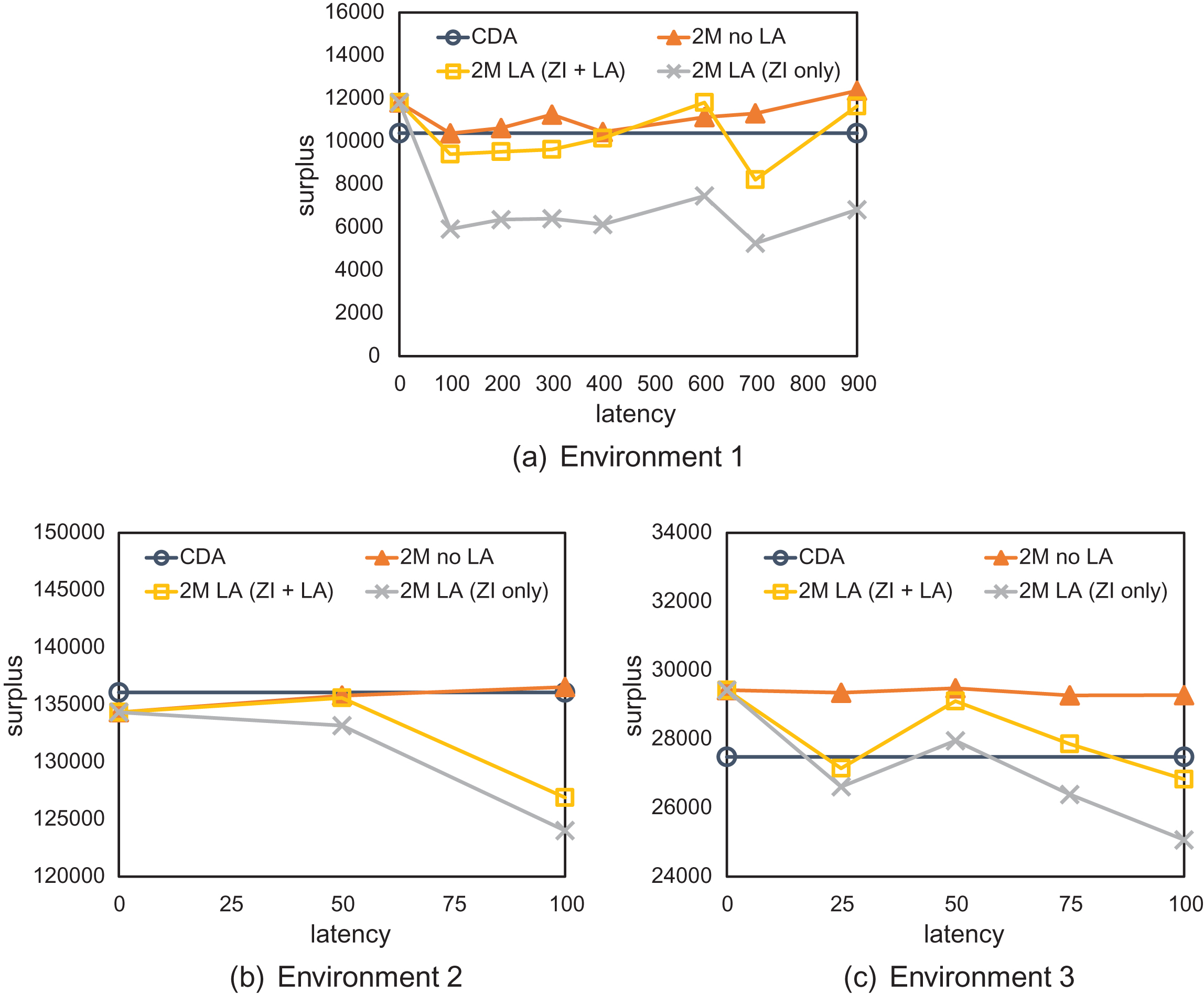
Figure 4 shows the total surplus, for the consolidated CDA and the two-market model with and without a latency arbitrageur, over multiple latency settings in the three environments. The total surplus of the two-market model without LA, as well as that of the single CDA market (an unfragmented continuous-time market), generally exceeds that of the two-market model with LA, whether or not the profits of LA are counted. This holds across the three environments. In other words, the latency arbitrageur takes surplus away from the background investors, and the amount it deducts exceeds the gross trading profit it accrues.
Fig.4
Total surplus in the two-market (2M) model, both with and without a latency arbitrageur, and in the consolidated CDA market, for the three environments. In the two-market model with LA, both the total surplus (ZI + LA) and background-trader surplus (ZI only) are plotted. Each point reflects the average over 50,000 simulation runs of the maximum-welfare equilibrium for each market configuration and latency setting.
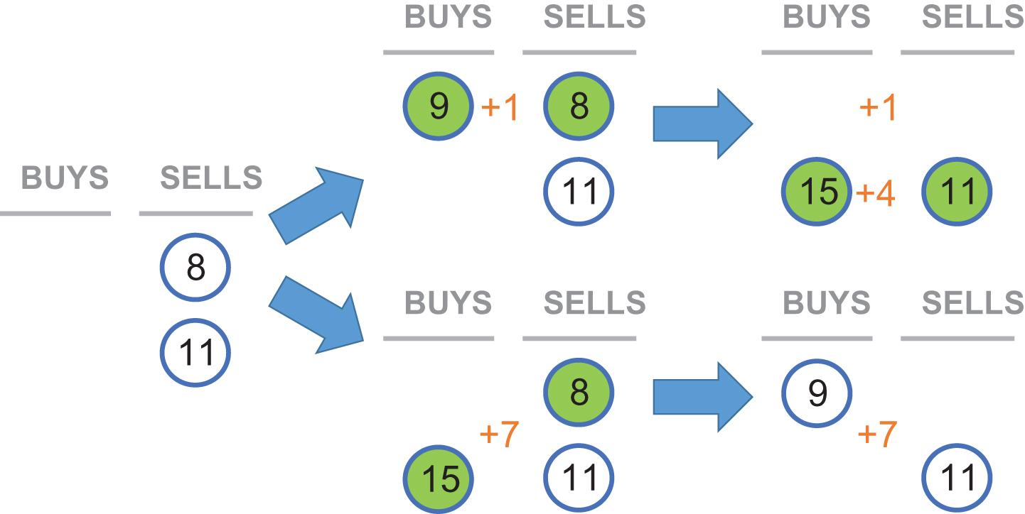
The intuition behind this result lies in differences in the orders selected to trade. Figure 5 demonstrates how changes in the order arrival sequence may lead to different levels of surplus. A continuous market will match two orders to trade immediately, regardless of whether this transaction improves allocative efficiency. The LA, by matching orders across the two fragmented markets, is prone to facilitate some inefficient trades that would not execute in the two-market model without latency arbitrage.
Fig.5
Welfare differences that arise from changes in order sequencing in continuous markets. The order book initially has two sell orders. Two buy orders arrive, with different sequencing, over the course of two time steps. In the top scenario, the buy order at price 9 arrives before the buy order at 15, resulting in total surplus of 5 from two trades (assuming traders submit orders priced at their valuations). In the bottom scenario, the buy order at price 15 arrives first, which results in a more efficient transaction (with a higher surplus of 7) than the alternate scenario. Each pair of green circles indicate orders that have matched and traded at a given moment in time.
In environment 1, LA significantly degrades efficiency in the two-market model, and total LA profit accounts for half of aggregate surplus once nonzero latency is introduced. Environments 2 and 3, however, have reduced mean reversion, which increases background traders’ risk of adverse selection and having the LA pick off their standing orders. As a result, background traders in these two environments shade more in response to the LA. This can be seen by higher Rmid values in the NE found. Prior work by Zhan and Friedman (2007) has shown that strategicallydetermined levels of bid shading can mitigate inefficient trades in CDAs. The infinitely fast arbitrageur immediately exploits arbitrage opportunities that arise from incorrectly routed orders; these LA trades tend to be inefficient, which contributes to the lower overall welfare observed in the two-market model with LA. Increased bid shading in the low mean reversion environments can alleviate some of these inefficiencies, which improves background-trader surplus and reduces LA profits.
7.2Effect of fragmentation on market efficiency
Note that when latency is zero, the two fragmented models and the CDA market in Fig. 4 are effectively identical. The NBBO is always correct if there is no delay, so it is not possible for any latency arbitrage opportunities to emerge. It follows that the various market configurations at zero latency produce similar total surplus in equilibrium. Some differences between the consolidated and fragmented models, however, may arise due to strategies with η < 1. In fragmented markets, the decision to submit executable orders is based on the current best quote in the trader’s assigned market, not the NBBO, leading to possibly different results between the two-market model and consolidated CDA, even at zero latency.
Consolidating the markets in a single CDA generally outperforms the fragmented market with LA in environments 1 and 2. This effect is muted in thinner markets when there are fewer trading opportunities, such as environment 3. As for the case without latency arbitrage, it may seem counterintuitive that welfare in the two-market model without LA is higher than in the consolidated CDA in some environments. It turns out that fragmentation can actually provide a benefit for continuous markets. The separated markets are less likely to admit inefficient trades (i.e., where both traders’ values fall on the same side of the longer-term equilibrium price) that arise due to the vagaries of arrival sequences (Wah and Wellman, 2013), as illustrated in Fig. 5. LA can defeat this benefit by ensuring that any orders that would match in the central CDA also trade in the fragmented case, albeit with LA rather than with a counterpart investor. This primarily applies when there are sufficient trading opportunities, as in environments 1 and 2. In a thicker market as in environment 2, fragmentation does not always boost surplus in the two-market model without LA, as there are many traders in each market who can act as counterparties for trade.
7.3Effect of LA and fragmentation on liquidity
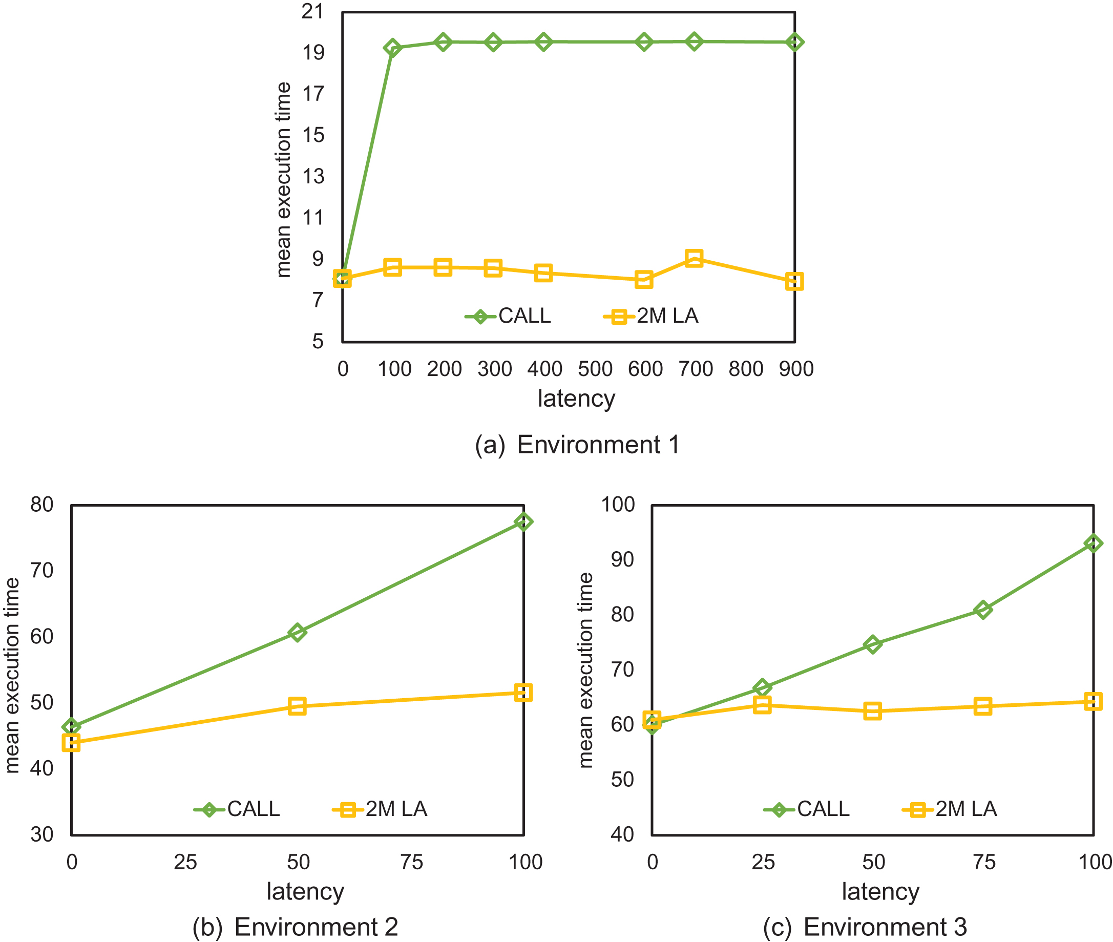
We also evaluate the effect of latency arbitrage on market liquidity, as measured via execution times and BID-ASK spreads. Figure 6 shows that execution time tends to be highest in the two-market model with LA. The fastest trade execution in environment 1 is achieved in the two-market model without LA, which differs from findings in the literature that trading at lower latencies improves overall execution time (Angel et al., 2011; Garvey and Wu, 2010; Riordan and Storkenmaier, 2012). This is largely due to the different strategies selected in equilibrium in this environment; traders tend to shade their bids less (i.e., Rmid is lower) in the fragmented model without LA, hence orders are more likely to execute sooner rather than later. The improvement in execution time is at best approximately 1–2 time steps, however, which is generally insignificant to non-HFtraders.
Fig.6
Execution time in the two-market (2M) model, both with and without a latency arbitrageur, and in the consolidated CDA market, for the three environments. Execution time is the difference between bid submission and transaction times. Each point reflects the average over 50,000 simulation runs of the maximum-welfare equilibrium for the market configuration and latency setting.
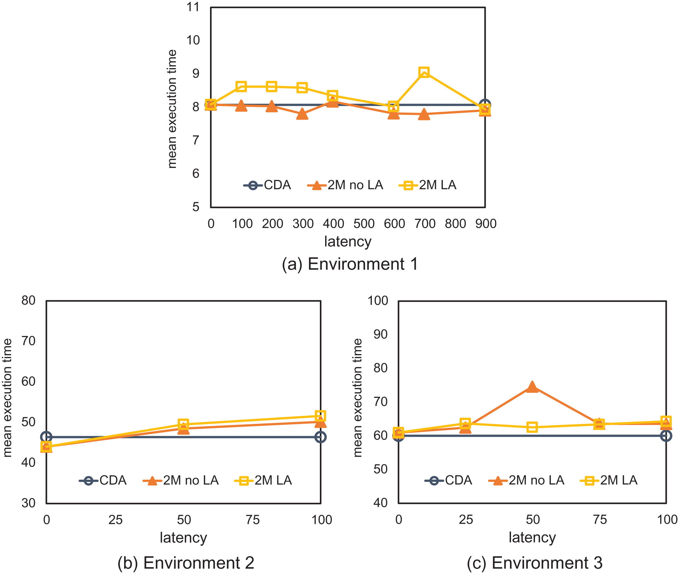
Traders in the other two environments, however, do not shade more in equilibrium in the two-market model without LA. In these cases, the fastest execution is achieved in the consolidated CDA, which makes sense given the absence of both communication latencies and thinness induced by fragmentation.
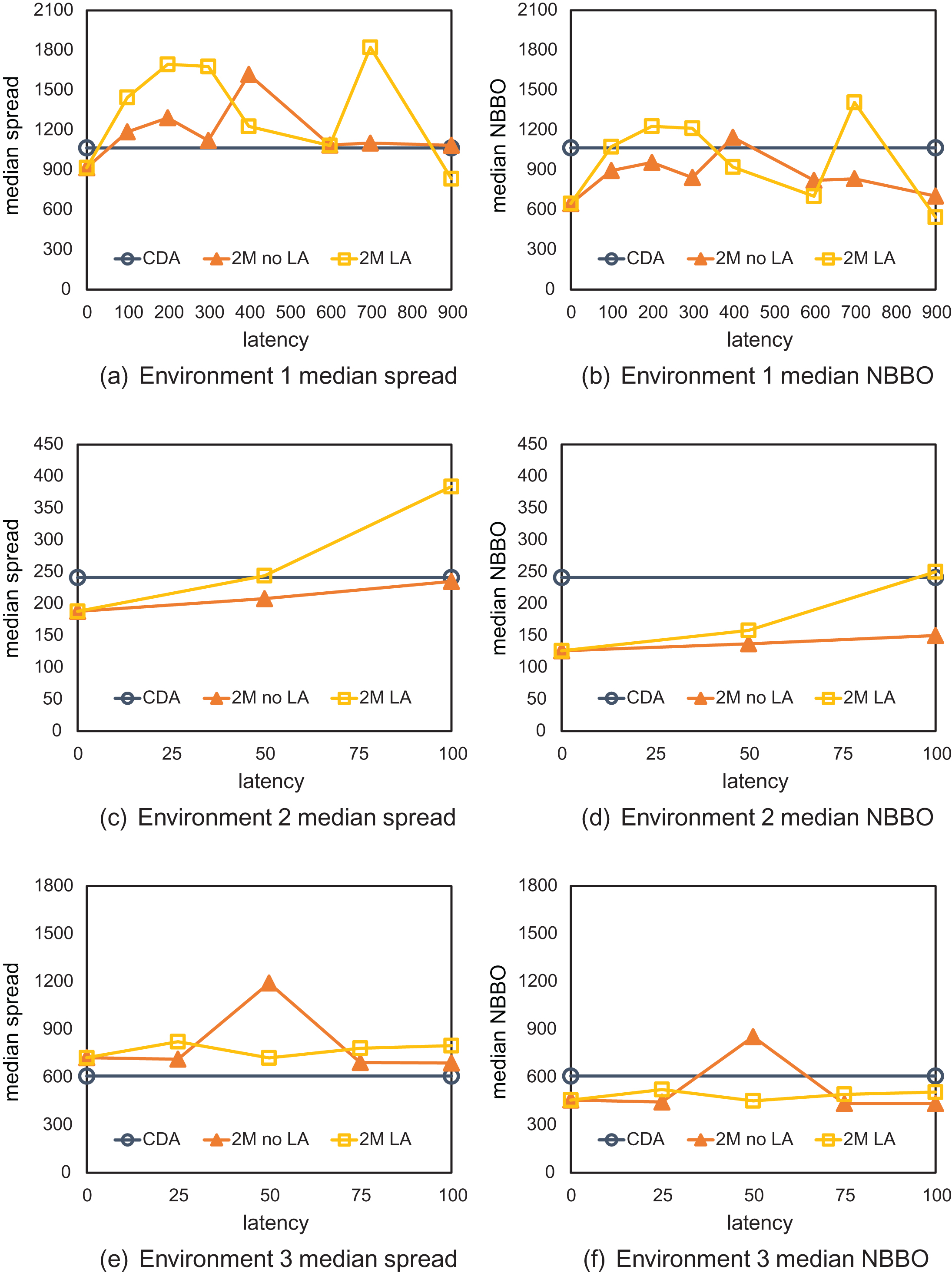
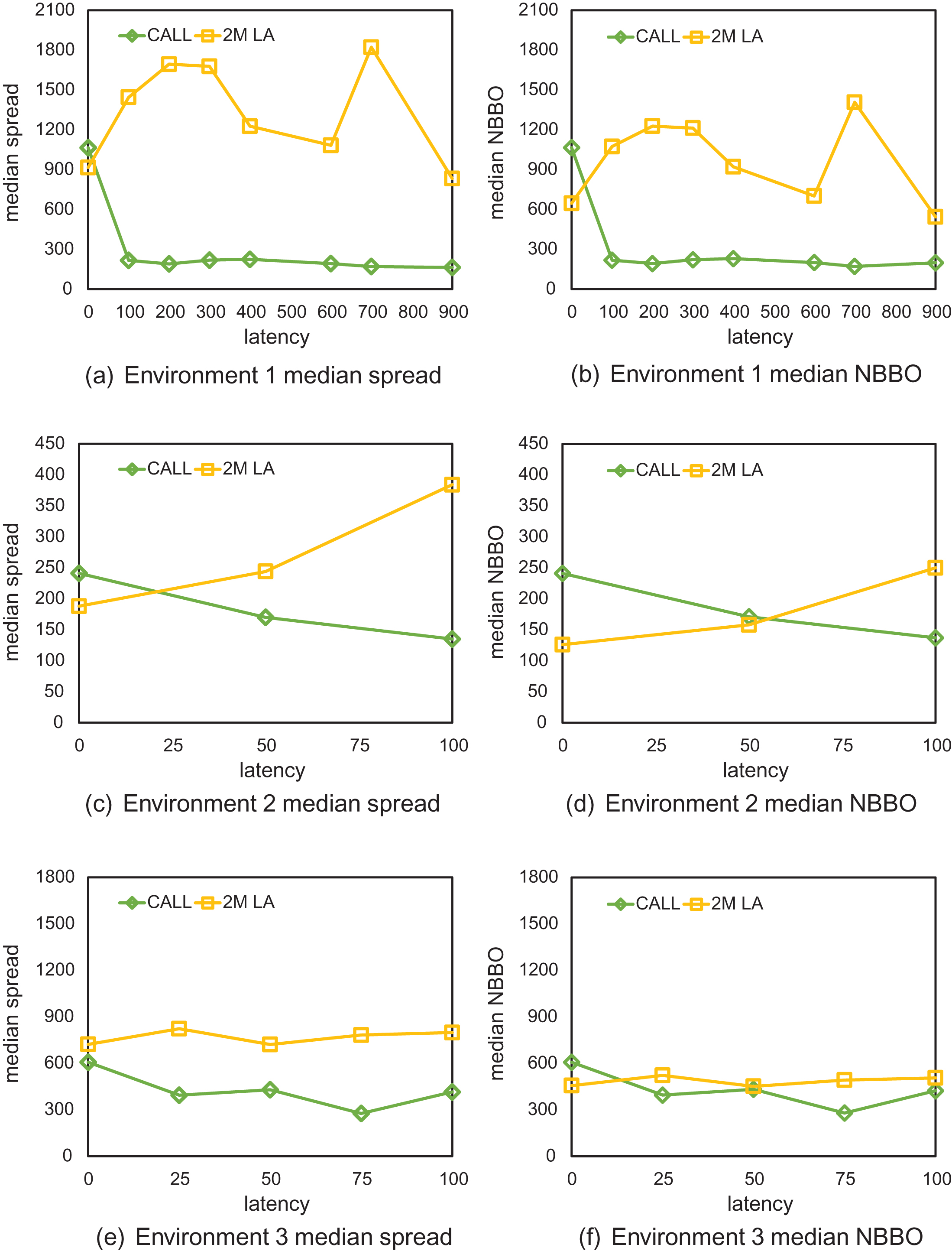
Spreads can also be viewed as a measure of liquidity, with tighter spreads corresponding to greater market liquidity. The widest spreads are generally in the two-market model with LA (Fig. 7). LA also slightly exacerbates NBBO spreads, which are generally narrower than spreads of individual markets. The increase in spread could reflect an implicit transaction cost responsible for part of the surplus reduction observed above.
Fig.7
Median spread and NBBO spread in the two-market (2M) model, both with and without a latency arbitrageur, and in the consolidated CDA market, for the three environments. Spread is the amount by which ASK exceeds BID. NBBO spread is the difference between BID and ASK of the NBBO quote. The spread at a given latency in each two-market configuration is the mean of the median spread in the two individual markets. Each point reflects the average over 50,000 simulation runs of the maximum-welfare equilibrium for the market configuration and latency setting.
7.4Effect of switching to a frequent call market
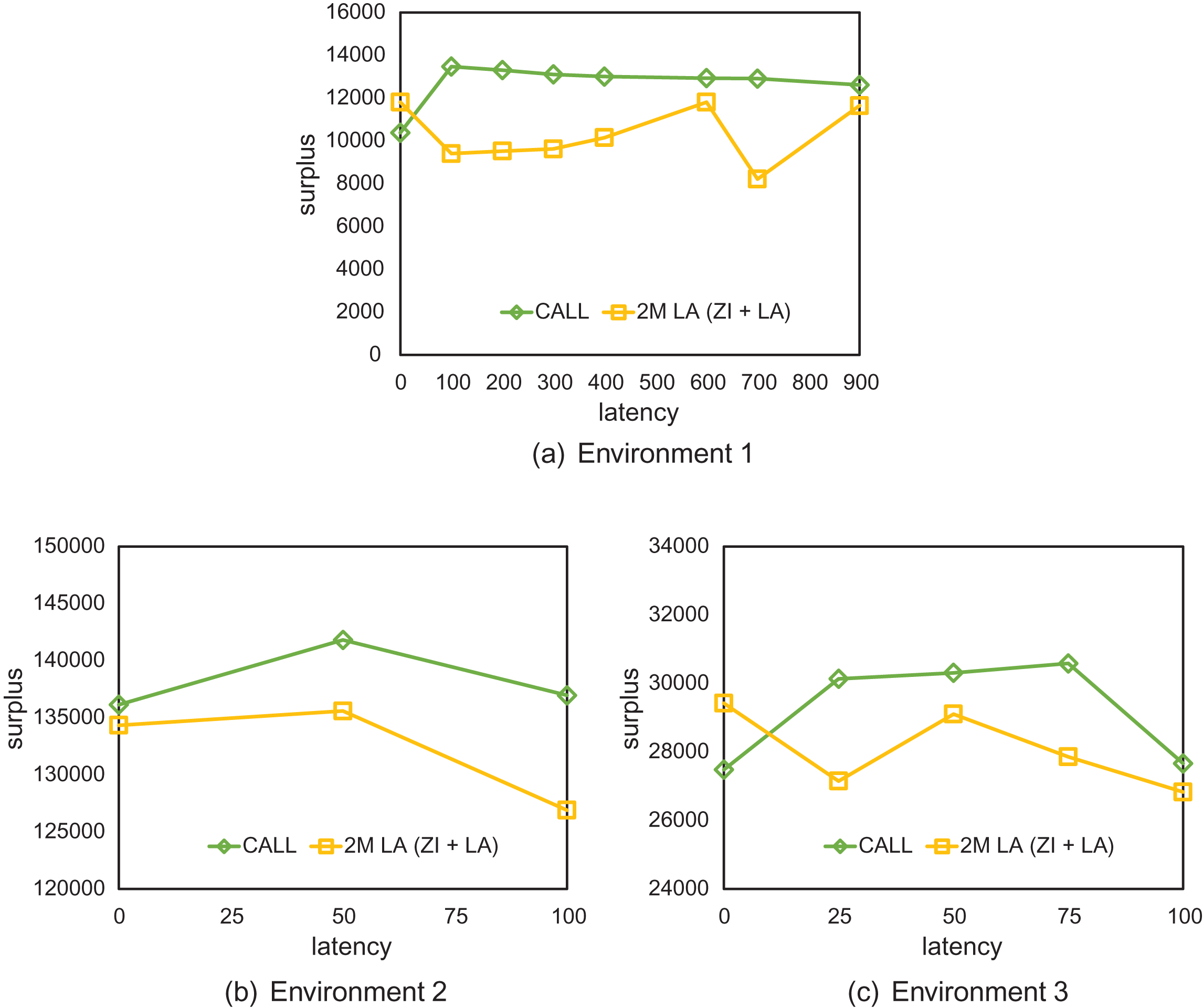
Lastly, we evaluate the effect of switching to a discrete-time frequent call market. In our frequent call market configuration, the latency setting dictates the clearing period. Figure 8 shows that the total surplus in the consolidated call market far exceeds that of the two-market model with LA, and the call market surplus is higher for all latency settings δ > 0 (there are only two market configurations at zero latency, the fragmented model without LA and the consolidated CDA). By aggregating orders over time, call markets perform a more informed clear. They increase the probability that trades occur between intra-marginal traders—those with private valuations inside the equilibrium price range—and thus are less prone to executing inefficient trades than CDAs (Gode and Sunder, 1997).
Fig.8
Total surplus for the consolidated frequent call market and the two-market (2M) model with LA, for the three environments. Each point reflects the average over 50,000 simulation runs of the maximum-welfare equilibrium for each market configuration and latency setting.
As shown in Fig. 9, the mean execution time in the consolidated call market is much higher than that of the two-market model with LA. Unsurprisingly, we find that execution time in the call market is higher than that observed in the other market configurations. As market clears occur less frequently in the call market, it takes longer for a bid to match and be removed from the order book. In environment 1, execution time in the frequent call market plateaus at approximately 20 time steps, which is equivalent to the average time between trader reentries. In the other two environments, the execution time in the call market increases monotonically with the length of the clearing interval, since traders reenter less frequently than the market clears. This tradeoff between discrete clearing and execution speed may not significantly affect investors if the frequent call market matches orders frequently, such as once everysecond.
Fig.9
Execution time for the consolidated frequent call market and the two-market (2M) model with LA, for the three environments. Each point reflects the average over 50,000 simulation runs of the maximum-welfare equilibrium for each market configuration and latency setting.
In Fig. 10, we observe that the tightest spread is realized in the consolidated call market, for all three environments. Spreads in the frequent call market are measured at the end of each market clear. They represent the market liquidity after orders have traded in each interval. Since the call market generally matches orders to trade more efficiently than the CDA, its spreads tend to be tighter. The median spread decreases to some degree with latency due to the accumulation of bids in the order book, which is indicative of greater liquidity in the market. The temporal aggregation in the consolidated call market is also responsible for similarly tight NBBOspreads.
Fig.10
Median spread and NBBO spread for the consolidated frequent call market and the two-market (2M) model with LA, for the three environments. Each point reflects the average over 50,000 simulation runs of the maximum-welfare equilibrium for each market configuration and latency setting.
7.5Relationship between transactions and surplus
Figure 11 shows the total number of transactions in each market configuration, for the three environments, averaged over all observations at a given latency. In all three environments, the total number of transactions in the consolidated CDA and the two-market model without LA are generally comparable, though slightly lower in the latter. This is consistent with our observations of surplus patterns in Fig. 4. The two-market model without LA results in higher surplus despite a reduction in number of transactions, indicating that each transaction in the fragmented model is associated with more surplus on average than in the consolidated CDA. The number of LA transactions does not increase with latency, although the number of arbitrage opportunities grows as the NBBO update delay increases. Since the background traders strategically respond to the presence of the LA by submitting executable orders over limit orders, they are less likely to be picked off by the LA.
Fig.11
Total number of transactions in each of the four market configurations for the three environments. In the two consolidated markets (call and CDA) and the two-market (2M) model without LA, there is no latency arbitrage so transactions only occur between ZI traders. The rightmost bar in each group of four shows the total number of transactions in the two-market model with LA, with the top portion of the stacked bar representing the number of LA transactions and the bottom portion representing the ZI transactions. Each bar reflects the average over 50,000 simulation runs of the maximum-welfare equilibrium for each market configuration and latency setting.
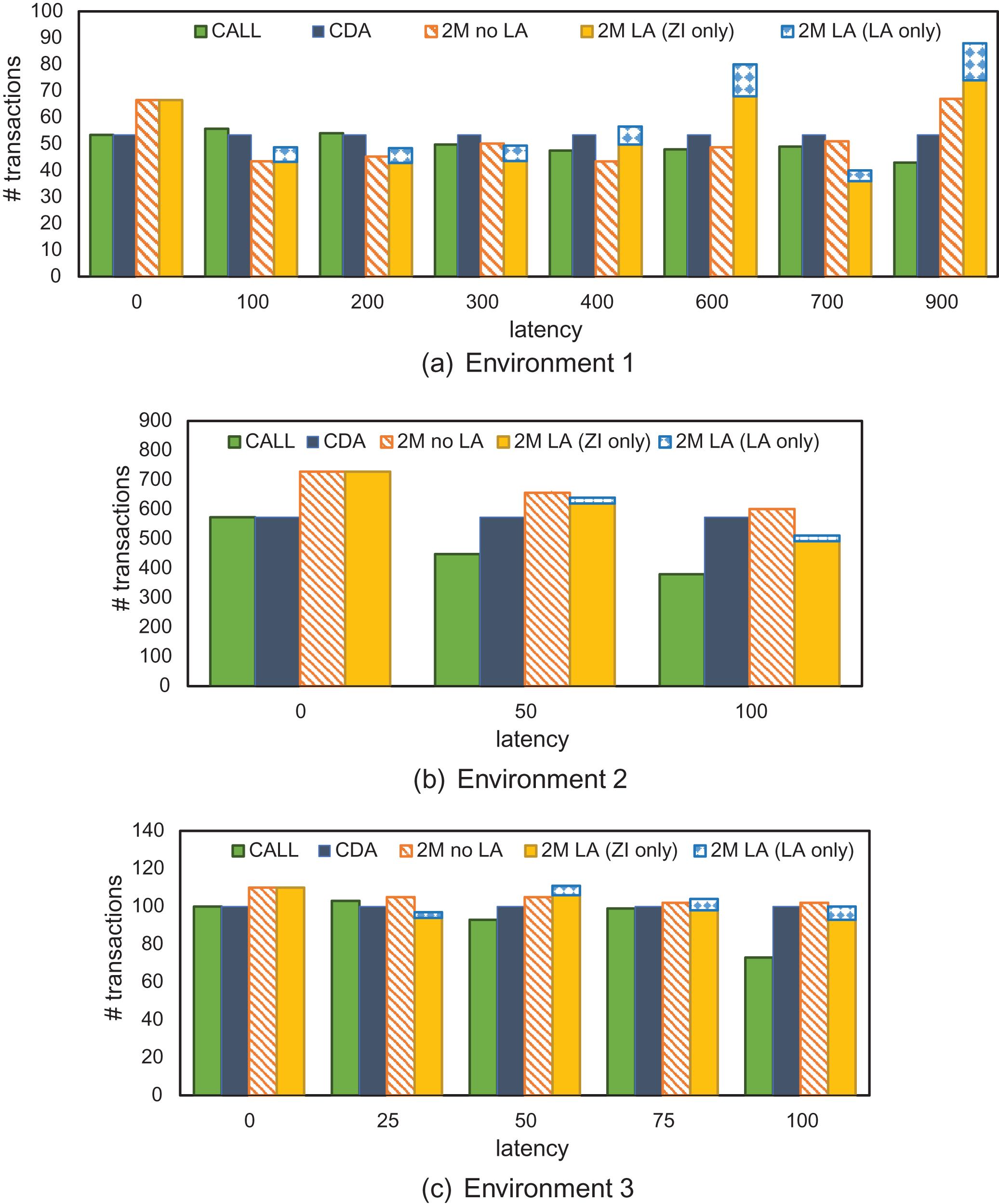
In addition, the highest number of trades for a market configuration at a given latency setting in environment 1 is generally (although not always) observed in the call market. This is a result of the reduced Rmid values observed in the call market equilibria; traders in the frequent call market tend to shade their bids less in equilibrium, and consequently are more likely to trade. In contrast, transaction volume is generally lower in the frequent call market in the low mean reversion environments. Given the corresponding surplus improvement (Fig. 4), this indicates that discrete-time clearing leads to higher surplus per trade.
8Conclusions
Our two-market model captures fragmentation in its simplest form, enabling our investigation of an important phenomenon in high-frequency trading: latency arbitrage. We implemented this model in a system combining agent-based modeling and discrete-event simulation. We employed empirical game-theoretic analysis to compute equilibria in games with variations in market structure and within three parametrically distinct environments, and we compared equilibrium outcomes in order to evaluate the interplay of latency arbitrage, market fragmentation, and market design, as well as their consequences for market performance.
Our results demonstrate that market efficiency in equilibrium is negatively affected by the actions of a latency arbitrageur, with no countervailing benefit in liquidity or any other measured market performance characteristic. Taking into consideration the substantial operational costs of the latency arms race would only amplify our conclusions about the harmful implications of this practice.
Somewhat counterintuitively, welfare in some environments of the fragmented model without LA is higher than in the consolidated CDA. It turns out fragmentation can provide a benefit in continuous markets, as the separation of markets mitigates the inefficient transactions that result from continuous trading. We find that the effect of fragmentation on liquidity varies depending on how traders strategically respond to the presence of LA.
Virtually all modern financial markets employ continuous trading, which enables speed-advantaged traders to exploit price differentials over fragmented markets. A frequent call market prevents high-frequency traders from gaining a meaningful latency advantage, thereby eliminating latency arbitrage opportunities and increasing surplus for background traders. Aggregating orders over small, regular time intervals provides efficiency gains over fragmented and continuous markets, and in fact these benefits appear to overshadow the gains attributable specifically to neutralizing latency arbitrage.
As with any simulation model, our results are valid only to the extent our assumptions capture the essence of real-world markets. Additional avenues for further study include examining the effect of more sophisticated HFT and background-trader strategies (such as those using historical information or responding to LA price signals), introducing other types of traders such as market makers, and further quantifying the impact of price discovery on efficiency.
Notes
1 Profit figures are considerably more uncertain than volume estimates. Kearns et al. (2010) present an interesting approach to derive an upper bound on HFT profits. Presumably the billions HFT firms invest annually in technology and infrastructure (Adler, 2012) represent a lower bound on gross trading profit.
2 Order activity at the temporal granularity of interest here is generally unavailable for public research, and it is unclear whether data on communication latencies and the end-to-end routing of orders among brokers and exchanges is available from any source. What high-frequency trading data does exist commercially is prohibitively expensive. Moreover, even full details on conceivably observable trading activity could not directly resolve counterfactual questions, such as the response of financial markets to possible shocks or the effects of alternative market rules and regulations.
3 With the exception of environment 1, the number of players N in the full game and the number of reduced-game players k are selected to ensure that the DPR definitions result in integer numbers of players. See the original paper by Wiedenbeck and Wellman (2012) for the complete definition of the number of reduced-game players when divisibility does not hold.
Acknowledgments
We are grateful for constructive suggestions from Jacob Abernethy, Michael Barr, Uday Rajan, and members of the Strategic Reasoning Group at the University of Michigan, along with an anonymous reviewer, leading to improvements in the substance and presentation of this work. This research was supported in part by grant IIS-1421391 from the US National Science Foundation.
References
1 | Adler J. , (2012) . Raging bulls: How Wall Street got addicted to light-speed trading, Wired Magazine 20: (9). |
2 | Aldridge I. , (2013) . High-Frequency Trading, second edn, Wiley. |
3 | Amihud Y. , Lauterbach B. , Mendelson H. , (2003) . The value of trading consolidation: Evidence from the exercise of warrants, Journal of Financial and Quantitative Analysis 38: (4), 829–846. |
4 | Amihud Y. , Mendelson H. , Lauterbach B. , (1997) . Market microstructure and securities values: Evidence from the Tel Aviv Stock Exchange, Journal of Financial Economics 45: (3), 365–390. |
5 | Angel J.J. , Harris L.E. , Spatt C.S. , (2011) . Equity trading in the 21st century, Quarterly Journal of Finance 1: (1), 1–53. |
6 | Arnuk S.L. , Saluzzi J.C. , (2012) . Broken Markets: How High Frequency Trading and Predatory Practices on Wall Street are Destroying Investor Confidence and Your Portfolio, FT Press. |
7 | Avellaneda M. , Stoikov S. , (2008) . High-frequency trading in a limit order book, Quantitative Finance 8: (3), 217–224. |
8 | Baldauf M. , Mollner J. , (2014) . High-frequency trade and market performance, Technical report, Stanford University Economics Department. |
9 | Banks J. , Carson II J.S. , Nelson B.L. , Nicol D.M. , (2005) . Discrete-Event System Simulation, fourth edn, Prentice Hall. |
10 | Baron M. , Brogaard J. , Kirilenko A. , (2012) . The trading profits of high frequency traders, Technical report, Commodity Futures Trading Commission. |
11 | Bennett P. , Wei L. , (2006) . Market structure, fragmentation, and market quality, Journal of Financial Markets 9: (1), 49–78. |
12 | Biais B. , Glosten L. , Spatt C. , (2005) . Market microstructure: A survey of microfoundations, empirical results, and policy implications, Journal of Financial Markets 8: (2), 217–264. |
13 | Blume M.E. , (2007) . Competition and fragmentation in the equity markets: The effects of Regulation NMS, Technical Report 02-07, The Rodney L. White Center for Financial Research, The Wharton School, University of Pennsylvania. |
14 | Bowley G. , (2010) . U.S. markets plunge, then stage a rebound, The New York Times. |
15 | Brogaard J. , (2010) . High frequency trading and its impact on market quality. Northwestern University Kellogg School of Management Working Paper. |
16 | Buchanan M. , (2009) . Meltdown modelling, Nature 460: (7256), 680–682. |
17 | Budish E. , Cramton P. , Shim J. , (2015) . The high-frequency trading arms race: Frequent batch auctions as a market design response, Quarterly Journal of Economics 130: (4), 1547–1621. |
18 | Cardella L. , Hao J. , Kalcheva I. , Ma Y.-Y. , (2014) . Computerization of the equity, foreign exchange, derivatives, and fixed-income markets, Financial Review 49: (2), 231–243. |
19 | Cassell B.-A. , Wellman M.P. , (2013) . EGTAOnline: An experiment manager for simulation-based game studies, in ‘Multi-Agent-Based Simulation XIII’, Vol. 7838 of Lecture Notes in Artificial Intelligence, Springer. |
20 | Chen S.-H. , Chang C.-L. , Du Y.-R. , (2012) . Agent-based economic models and econometrics, Knowledge Engineering Review 27: (2), 187–219. |
21 | Cohen S.N. , Szpruch L. , (2012) . A limit order book model for latency arbitrage, Mathematics and Financial Economics 6: (3), 211–227. |
22 | Das R. , Hanson J.E. , Kephart J.O. , Tesauro G. , (2001) . Agent-human interactions in the continuous double auction, in 17th International Joint Conference on Artificial Intelligence, pp. 1169–1176. |
23 | De La Merced M.J. , (2013) . Shutdown at Nasdaq is traced to software, The New York Times. |
24 | Ding S. , Hannah J. , Hendershott T. , (2014) . How slow is the NBBO? A comparison with direct exchange feeds, Financial Review 49: (2), 313–332. |
25 | Farmer J.D. , Foley D. , (2009) . The economy needs agent-based modeling, Nature 460: (7256), 685–686. |
26 | Farmer J.D. , Skouras S. , (2012) . Review of the benefits of a continuous market vs. randomised stop auctions and of alternative priority rules (policy options 7 and 12). |
27 | Foucault T. , Kozhan R. , Tham W.W. , (2015) . Toxic arbitrage, Technical Report No. FIN-2014-1040, HEC Paris. |
28 | Friedman D. , (1993) . The double auction market institution: A survey, in D. Friedman & J. Rust, eds, The Double Auction Market: Institutions, Theories, and Evidence, Addison-Wesley, pp. 3–25. |
29 | Gammeltoft N. , Griffin D. , (2013) . Goldman Sachs said to send stock-option orders by mistake, Bloomberg. |
30 | Garvey R. , Wu F. , (2010) . Speed, distance, and electronic trading: New evidence on why location matters, Journal of Financial Markets 13: (4), 367–396. |
31 | Gode D.K. , Sunder S. , (1993) . Allocative efficiency of markets with zerointelligence traders: Market as a partial substitute for individual rationality, Journal of Political Economy 101: (1), 119–137. |
32 | Gode D.K. , Sunder S. , (1997) . What makes markets allocationally efficient? Quarterly Journal of Economics 112: (2), 603–630. |
33 | Goettler R.L. , Parlour C.A. , Rajan U. , (2009) . Informed traders and limit order markets, Journal of Financial Economics 93: (1), 67–87. |
34 | Goldstein M.A. , Kumar P. , Graves F.C. , (2014) . Computerized and high-frequency trading, The Financial Review 49: (2), 177–202. |
35 | Government Office for Science, London. 2012. Foresight: The future of computer trading in financial markets, Technical report. |
36 | Hanson T.A. , (2012) . The effects of high frequency traders in a simulated market, in ‘Midwest Finance Association Annual Meeting’. |
37 | Hasbrouck J. , Saar G. , (2013) . Low-latency trading, Journal of Financial Markets 16: (4), 646–679. |
38 | Hendershott T. , Jones C.M. , Menkveld A.J. , (2011) . Does algorithmic trading improve liquidity? Journal of Finance 66: (1), 1–33. |
39 | Industry Super Network. 2013. Toward a fairer and more efficient share market: Frequent sealed bid call auctions with random durations, Technical report. ISN Research Report. |
40 | Jacobs B.I. , Levy K.N. , Markowitz H.M. , (2004) . Financial market simulation, Journal of Portfolio Management 30: (5), 142–152. |
41 | Jarrow R.A. , Protter P. , (2012) . A dysfunctional role of high frequency trading in electronic markets. International Journal of Theoretical and Applied Finance 15: (3), 1250022-1–1250022-15. |
42 | Kalay A. , Wei L. , Wohl A. , (2002) . Continuous trading or call auctions: Revealed preferences of investors at the Tel Aviv Stock Exchange, Journal of Finance 57: (1), 523–542. |
43 | Kearns M. , Kulesza A. , Nevmyvaka Y. , (2010) . Empirical limitations on highfrequency trading profitability, Journal of Trading 5: (4), 50–62. |
44 | LeBaron B. , (2004) . Building the Santa Fe artificial stock market, in Luna F., Tierna P. & Perrone A., eds, ‘Agent-Based Economics: Theory, Languages and Experiments’, Routledge Publishing. |
45 | LeBaron B. , (2006) . Agent-based computational finance, in Tesfatsion L. & Judd K.L., eds, ‘Handbook of Agent-Based Computational Economics’, Elsevier, pp. 1187–1233. |
46 | LeBaron B. , Arthur W.B. , Palmer R. , (1999) . Time series properties of an artificial stock market, Journal of Economic Dynamics & Control 23: (1), 1487–1516. |
47 | Lee W.B. , Cheng S.-F. , Koh A. , (2011) . Would price limits have made any difference to the ‘Flash Crash’ on May 6, 2010? Review of Futures Markets 19: , 55–93. |
48 | Lewis M. , (2014) . Flash Boys: A Wall Street Revolt, W.W. Norton & Company. |
49 | McPartland J. , (2013) . Recommendations for equitable allocation of trades in high frequency trading environments, Technical report, Federal Reserve Bank of Chicago. |
50 | Mehta N. , (2012) . Nasdaq chief blames software for delay in Facebook debut, Bloomberg. |
51 | Mendelson H. , (1987) . Consolidation, fragmentation, and market performance, Journal of Financial and Quantitative Analysis 22: (2), 189–207. |
52 | O’Hara M. , Ye M. , (2011) . Is market fragmentation harming market quality? Journal of Financial Economics 100: (3), 459–474. |
53 | Palmer R.G. , Arthur W.B. , Holland J.H. , LeBaron B. , Tayler P. , (1994) . Artifical economic life: A simple model of a stock market, Physica D: Nonlinear Phenomena 75: (1), 264–274. |
54 | Pancs R. , (2013) . Comparing market structures: Allocative and informational efficiencies of continuous trading, periodic auctions, and dark pools, Technical report, Department of Economics, University of Rochester. |
55 | Patterson S. , (2014) . High-speed stock traders turn to laser beams. The Wall Street Journal. |
56 | Pellizzari P. , Dal Forno, A. , (2007) . A comparison of different trading protocols in an agent-based market, Journal of Economic Interaction and Coordination 2: (1), 27–43. |
57 | Raberto M. , Cincotti S. , (2005) . Modeling and simulation of a double auction artificial financial market, Physica A Statistical Mechanics and its Applications 355: (1), 34–45. |
58 | Riordan R. , Storkenmaier A. , (2012) . Latency, liquidity and price discovery, Journal of Financial Markets 15: (4), 416–437. |
59 | Schneider D. , (2012) . The microsecond market, IEEE Spectrum 49: (6), 66–81. |
60 | Schwartz R.A. , Peng L. , (2013) . Market makers, in ‘Encyclopedia of Finance’, Springer, pp. 487–489. |
61 | Securities and Exchange Commission. 2005. ‘Regulation NMS’. 17 CFR Parts 200, 201, 230, 240, 242, 249, 270. |
62 | Securities and Exchange Commission. 2013. In the matter of Knight Capital Americas LLC, order instituting administrative and cease-and-desist proceedings, Release 70694. |
63 | Sellberg L.-I. , (2010) . Using adaptive micro auctions to provide efficient price discovery when access in terms of latency is differentiated among market participants, Technical report, Cinnober Financial Technology AB. |
64 | Sparrow C. , (2012) . The failure of continuous markets, Journal of Trading 7: (2), 44–47. |
65 | Thurner S. , Farmer J.D. , Geanakoplos J. , (2012) . Leverage causes fat tails and clustered volatility, Quantitative Finance 12: (5), 695–707. |
66 | Wah E. , (2016) . How prevalent and profitable are latency arbitrage opportunities on U.S. stock exchanges? SSRN Electronic Journal. |
67 | Wah E. , Wellman M.P. , (2013) . Latency arbitrage, market fragmentation, and efficiency: A two-market model, in 14th ACM Conference on Electronic Commerce, pp. 855–872. |
68 | Webb R.I. , Muthuswamy J. , Segara R. , (2007) . Market microstructure effects on volatility at the TAIFEX, Journal of Futures Markets 27: (12), 1219–1243. |
69 | Wellman M.P. , (2006) . Methods for empirical game-theoretic analysis (extended abstract), in 21st National Conference on Artificial Intelligence, pp. 1552–1555. |
70 | Wellman M.P. , (2009) . Countering high-frequency trading, http://strategicreasoning.org/countering-high-frequency-trading/ |
71 | Wellman M.P. , (2011) . Trading Agents, Morgan & Claypool. |
72 | Wheatley M. , (2010) . We need rules to limit the risks of superfast trades. Financial Times. |
73 | Wiedenbeck B. , Wellman M.P. , (2012) . Scaling simulation-based game analysis through deviation-preserving reduction, in 11th International Conference on Autonomous Agents and Multiagent Systems, pp. 931–938. |
74 | Zhan W. , Friedman D. , (2007) . Markups in double auction markets, Journal of Economic Dynamics and Control 31: (9), 2984–3005. |

