
Natural time analysis in financial markets
Abstract
In this paper we introduce natural time analysis in financial markets. Due to the remarkable results of this analysis on earthquake prediction and the similarities of earthquake data to financial time series, its application in price prediction and algorithmic trading seems to be a natural choice. This is tested through a trading strategy with very encouraging results.
Introduction
It’s a widespread belief that economic systems, such as financial markets, constitute one of the most vivid and rich example of complex systems (Mantegna and Stanley, 2000; Sornette, 2002, 2003, 2009; Yan et al., 2012; Preis et al., 2012; Münnix et al., 2012; Gvozdanovic et al., 2012; Borland, 2005). Complex systems are governed by dynamic characteristics which are founded on common and well established principles used to describe a great variety of scientific and technological approaches of different types of natural, artificial and social systems (Tsallis, 2009; Bar-Yam, 1997; Picoli Jr et al., 2007; Sornette and Helmstetter, 2002; Abe and Suzuki, 2004; Fukuda et al., 2003; Peters et al., 2001).
In order to comprehend the behaviour of financial markets and acquire a deeper knowledge of the rules which govern them, experience is drawn from the study of complex systems in diverse scientific fields. One of these fields is the field of geophysics and earthquake prediction. A lot of articles have contributed to the attempt of showing the similarities of the dynamic characteristics of earthquakes to financial markets (Petersen et al., 2010; Sornette, 2002; Bhattacharyya et al., 2007; Chakrabarti et al., 2008). As a representative example, it is argued that exchange-traded stock prices follow the dynamics of built-up and release stress, similar to earthquakes (Andersen et al., 2011). Moreover, the distribution of market volatility before and after a stock market crash is well described by the Gutenberg-Richter law, which reflects the scale-invariance and self-similarity of the underlying dynamics by a robust power-law relation (Sarlis et al., 2010; Varotsos et al., 2004). Finally, the cascade of volatility “aftershocks” triggered by the “main financial shock” is quantitatively similar to earthquakes, which have been described by three empirical laws, the Omori law, the productivity law and the Bath law (Petersen et al., 2010).
The aforementioned suggests that methods based on knowledge of earthquakes’ studies seems to be very promising in analysing the dynamics of financial markets and in predicting their evolution.
In the present paper, a new method for analysing financial markets with the help of Natural time analysis is proposed. The prime pillar of this theory is Natural time χ (Varotsos et al., 2001), a new frame for understanding the timing of the events, which can help us to analyse financial time series and reveal hidden dynamic characteristics. Moreover, the applicability of this theory to financial markets is demonstrated via the development and the implementation of a trading strategy.
Natural time analysis is a well established theory which has been applied successfully in prediction of earthquakes (in terms of time and magnitude) for more than ten years including the strongest earthquake that occurred in Greece on 14 February 2008 (Varotsos et al., 2007; Sarlis et al., 2008). Natural time enables the determination of the occurrence time of an impending major earthquake (Varotsos et al., 2011b) since it can identify when a complex system approaches a critical point (Varotsos et al., 2011c). With Natural time analysis we are also able to forecast the trajectory of dynamical models and systems (Ising model, OFC model) (Sarlis et al., 2011) as well as their transitions to a critical regime.
The rest of this article is constructed as follows. In Section 2 the concept of Natural time and its basic features is presented. In Section 3 it is shown how Natural time can be applied in financial time series. In Section 4 a trading strategy based on this is applied on major financial markets (major FX pairs, DJIA stocks). Also a portfolio implementation of this strategy on the stocks of S & P500 index shows that this theory can give very promising results. Finally, in Section 5 conclusions follow.
2Natural time
Conventional time is modelled as the continuum
2.1Definition of Natural time
Specifically, in a time series comprising of N events, the Natural time is defined as:
(1)
In Natural time analysis we are concerned about the evolution of the pair of two quantities (χk, Qk), where χk is the Natural time as aforementioned, and Qk is a quantity proportional to the “energy” of the k-th event. “Energy” constitutes a scientific definition which is really difficult to describe with one single comprehensive definition because of its many forms. Depending on the application, “energy” can take one of the usual forms encountered in physics or can be a measure suitable to the modelling purposes. For example in earthquake prediction, Qk stands for the duration of the k-th seismic electric signal (SES)1 (Varotsos et al., 2008). In detection of syndrom of Sudden Cardiac Death (SCD) we use the RR2 interval as Qk. In other Complex systems, such as Olami-Feder-Christensen (OFC) model (Olami et al., 1992), the size of avalanche is used as a quantity proportional to the “energy” (Qk) (Varotsos et al., 2011c).
In the standard rebound theory of earthquakes, elastic deformation energy3 is gradually stored in the crust of earth. As rocks on opposite sides of a fault are subjected to force and shift, they accumulate energy and slowly deform until their internal strength threshold is exceeded. This is the critical point at which energy is suddenly released in an earthquake. In other words, earthquake is a recurrent phenomenon which is a result of a continuous built-up stress and release process of the tectonic plates of the earth.
On the other hand, Andersen et al. (2011) show that world’s stock exchanges follow the dynamics of build-up and release of stress and they have a non-linear threshold response to events, similar to earthquakes. The non-linear response based on change blindness, a phenomenon in which humans (traders in this case) react disproportionally to big changes, results in only large changes to be taken into account whereas small changes go unnoticed.
A key principle in finance states that as new information is revealed, it immediately becomes reflected in the price of an asset and thereby loses its relevance (Famma, 1969). As a consequence, focusing initially on stock indices, stress (elastic deformation energy) enters the system because of price movements of the indices. The idea is that a large (eventually cumulative) price movement of a given stock index can induce stresses on other stock indices world-wide to follow its price movement. Similar to the BK model of earthquakes (Burridge and Knopoff, 1967), we assume a “stick-slip” motion of the indices so that only a large (eventually cumulative) movement of a given index has a direct impact in the pricing of the remaining indices world-wide. In this line of thinking, “price-quakes” can happen in the financial system as cascades of big price movements (Andersen et al., 2011).
Inspired by the aforementioned, we make the assumption that price can be a natural choice for a quantity proportional to energy. Various functions of price, price trend, volume or a suitable combination of them could be possible canditates as well. The selection depends on the application and the objectives pursued.
Equivalently with Qk, we consider the quantities:
(2)
(3)
2.2The normalized power spectrum Π (ω) and the variance κ1 of Natural time
Considering the evolution of the pair (χk, Qk), we define the function:
(4)
(5)
Using (5) we compute the normalized power spectrum Π (ω) as
(6)
According to probability theory (Varotsos et al., 2011a, 2002), for natural frequencies φ (smaller than 0.5), Π (ω) switches to a characteristic function of the probability pk. For small values of ω, we consider its Taylor expansion around 0:
(7)
(8)
The quantity κ1 corresponds to the variance of Natural time χ. Taking into account Equations (5) and (8) and along with the fact that Φ (0) =1, we find (Varotsos et al., 2005):
(9)
(10)
(11)
(12)
(13)
(14)
2.3Uniform distribution in Natural time
A fundamental application of Natural time is the paradigm of the uniform distribution. The most common application of this is the emission of uncorrelated bursts of energy Qk. In this case the expected pk is E (pk) =1/N.
We define the uniform distribution:
(15)
For N → ∞, the PDF p (χ) tends to the PDF of uniform distribution, loosely written as p (χ) =1.
Then, we evaluate the mean value of Natural time:
(16)
For N → ∞, p (χ) =1 and pn = 0. Using Equation (15), the variance κ1 of Natural time is:
(17)
3Methodology
3.1Analysing financial time series with Natural time
We assume that quantity (Qk), in which “market’s energy” is reflected, is the price of the market. Based on this assumption we consider the closing price of financial time series in the chosen time frame (time frames can be based on one minute, five minutes, daily, etc.). Usually the closing price is chosen to be the representative price of the chosen frame, as it is argued that it encapsulates all the available information (Famma, 1969), especially in popular time frames such as daily, monthly or yearly, but the analysis can be performed on any other price (e.g. open, high, low, etc.).
As a first step, we normalize the data to zero mean and unit standard deviation and then we add the minimum value in order to ensure that each point is greater or equal to zero (Qk should be a positive quantity). For each value of the normalized data (Qk) we assign the index of its occurrence (χk).
Then, we calculate the evolution of variance of Natural time χ, κ1 (as a function of conventional time) using overlapping rolling windows with step 1 of the past L values of the data (1 : L, 2 : L + 1, . . . , L : L + n - 1), where n is the number of data under study.
An illustrative example of one minute data of EUR/USD (date:09/21/2012 from 07:50 until 18:07) with the evolution of the data and the evolution of variance κ1 with a rolling window of 300 values exists in Fig. 2.
In the example above we randomly shuffle the EUR/USD data and recalculate the variance of κ1 as shown in Fig. 3. Upper panel shows the shuffled data and the lower panel shows the evolution of variance of κ1, both in conventional time. We observe that the variance of Natural time κ1 in Fig. 3 displays a different trajectory in comparison with the evolution of κ1 in Fig. 2. In particular κ1, after initial fluctuations, stabilizes to a value around κ1 = κu = 0.083 which is indicative for the case of uniform distribution as shown is subsection 2.3. This reveals that the exact sequence of the events (Qk) and not the events themselves, determine the evolution of variance κ1. This is very encouraging for the selection of the variance of κ1 as a candidate metric for developing trading strategies.
Focusing on Fig. 2, we divide κ1 curve into segments based on local minima and maxima. Each segment starts from the detection of a local minimum (maximum) and ends up to the detection a local maximum (minimum) as shown in Fig 4.
In order to ensure the detection of local extrema we need to track the κ1 curve’s evolution in the right neighbourhood of the local extrema which inevitably introduces a time lag. That is why the green and red boxes are displaced from five to ten minutes (basic time unit in our case is the minute) relative to the actual points of minima (maxima). This allows us to track the evolution of both time series, EUR/USD and κ1 curve, simultaneously in each separate segment.
We observe that the division of upward and downward trends of κ1 curve coincides with upward and downward trends of EUR/USD (green and red boxes respectively).
We also see that variance of Natural time χ spots local minimums or maximums on the data. This seems to be unexpected but welcomed since the introduction of a short lag for local extrema detection is unavoidable. Actually κ1 predicts the minimum or maximum of data and that makes Natural time analysis’ prediction of trend to coincide with the actual one. So if we detect a local minimum(maximum) in the evolution of κ1 in conventional time, we are able to infer that it signifies a forthcoming upward(downward) trend in the original data, from which κ1 is calculated.
4Trading strategies based on Natural time
This particular characteristic of Natural time analysis allows us to create trading strategies with acceptable risk return characteristics. The key for a trading strategy lies in the successful determination of future trends in the market. As shown in Fig. 4, the blue κ1 curve depicts downward (upward) trend and helps us to divide the time series to short(long)areas.
A natural extension to this, is the simultaneously use of two, instead of one, different time windows. For example, a large one (Lb = 300) and a smaller one (Ls = 30) as it is shown in Fig. 5. The use of multiple time windows allows us to consider data variations that emerge in different time scales simultaneously. So, with the introduction of the second (smaller) time window we manage to compartmentalize the original data in a deeper level, taking into account the data microstructure characteristics.
The core of this strategy is the evolution of variance of Natural time κ1 in two time windows. Specifically, κ1 curve (blue), which comes from the larger time window, is used as an indicator for an upward(downward) trend and helps us to divide the time series into short(long) trading areas. The κ1 curve (green) which comes from the smaller time window serves as a position indicator in the market.
In Fig. 5, a local maximum (minimum) of the blue curve signifies the upward trend until the next local minimum (maximum) of the same curve. During this period, when a local maximum (minimum) of the green curve is detected, the opening of a short (long) position is suggested. This position will be closed when the next minimum (maximum) of the green curve is identified.
The above strategy suggests a simple example how the Natural time analysis can be used in order to profit from the markets.
This strategy has also been implemented on major currency pairs (Table 1) and on the 30 stocks of Dow Jones Industrial Average Index (DJIA) (Table 2).
We see that this strategy delivers results that have a stable profitability whereas its overall return can be characterized as promising. For all the major currency pairs the returns were positive for the whole trading period (2010–2013) and the equal weight portfolio of currency pairs has positive results for every trading year. In addition only 7 out of 30 stocks of the DJIA delivered negative results for the whole trading period (2011–2014). Another significant feature is that the results are uncorrelated with the returns and with the volatility of DJIA. To show this an equal weight portfolio with the stocks of DJIA based on this strategy is implemented. The results are shown in Table 3.
The above strategy was also implemented and back tested to the universe of the stocks of S & P500 index and a portfolio of 20 stocks was constructed with the help of a ranking algorithm. The algorithm took into consideration the persistence and the constant behaviour of stock returns in various time frames and their interaction with strategy characteristics (returns, max draw down, percentage of winning trades, etc.). Out-of-sample portfolio were run (for one trading year) and the results are shown in Table 4.
As the results show, strategy’s portfolio is characterized by promising metrics (satisfactory yearly returns, index out performance in five out of six years and acceptable VAR and expected value at risk of 1.2% (on average) at 95% significance level4. Agian the portfolio’s results have no correlation with the returns of S & P500 or with volatility of S & P500 (Table 5).
It is also important to note that in this strategy we do not use any traditional trading rules, such as trailing stops, stop loss, etc. We only use signals which are generated exclusively from Natural time analysis in stock’s time series in order to take our trading decisions. This is done intentionally so that the strength of the analysis to be shown5.
5Conclusions
A new way of analysing financial time series based on Natural time analysis, a theory of physics with remarkable results on earthquake prediction has been proposed. This theory treats time with a different manner in contrast with the standard model of continuous time. In this framework, the implementation of variance of Natural time κ1 in a time serie results in successful prediction of the upcoming trend. This feature can be used to develop winning trading strategies based on variance of Natural time κ1. Since Natural time analysis was developed for physical phenomena, strategies based on this theory are difficult to be characterized with the usual terms found in the finance jargon like trending strategies, volatility strategies, etc. Another important feature of this is that it is possible to construct profitable trategies based on Natural time that give results uncorellated to the returns and to the volatility of indices. This is very useful for reasons of diversification. We suspect that Natural time analysis has also many other useful applications in finance. Our future work will focus on phases of the markets, their transitions form one phase to another and the finding of stationary regimes in financial time series (choppy market periods) via the parameters of Natural Time. In an upcoming article we show how Natural time analysis, in a more microstucture level, can reveal information for impending large financial events using the variability of κ1 and how this information can be used for the production of trading strategies.
Notes
1 SES: Low frequency ≤ 1Hz electric signals that precede earthquakes.
2 RR is (beat-to-beat) interval time serie of an electrocardiogram.
3 Elastic energy is the potential mechanical energy stored in the configuration of a material or physical system as work is performed to distort its volume or shape. Elastic energy occurs when objects are compressed and stretched, or generally deformed in any manner (Landau and Lifshitz, 1986).
4 Other popular metrics useful for evaluating algorithms such as average winning to losing days, average size of winning and losing trade, etc. are available from the authors upon request.
5 Despite the conventional belief, trailing stops do not necessarily improve the results of a strategy.
References
1 | Abe S. , Suzuki N. , (2004) . Statistical similarities between internetquakes and earth-quakes. Physica D: Nonlinear Phenomena 193: , 310–314. |
2 | Andersen J.V. , Nowak A. , Rotundo G. , Parrott L. , Martinez S. , (2011) . price-quakes shaking the world’s stock exchanges. PloS One 6: , e26472. |
3 | Bar-Yam Y. , (1997) . Dynamics of complex systems. |
4 | Bhattacharyya P. , Chatterjee A. , Chakrabarti B.K. , (2007) . A common mode of origin of power laws in models of market and earthquake. Physica A: Statistical Mechanics and its Applications 381: , 377–382. |
5 | Borland L. , (2005) . Long-range memory and nonextensivity in financial markets. Euro-Physics News 36: , 228–231. |
6 | Burridge R. , Knopoff L. , (1967) . Model and theoretical seismicity. Bulletin of the Seismological Society of America 57: , 341–371. |
7 | Chakrabarti B.K. , Chatterjee A. , Bhattacharyya P. , (2008) . Two-fractal overlap time series: Earthquakes and market crashes. Pramana 71: , 203–210. |
8 | Famma E. , (1969) . Efficient capital markets: A review of theory and empirical work. Journal of Finance 25: , 383–417. |
9 | Fukuda K. , Amaral L.N. , Stanley H. , (2003) . Similarities between communication dynamics in the internet and the autonomic nervous system. EPL (Europhysics Letters) 62: , 189. |
10 | Gvozdanovic I. , Podobnik B. , Wang D. , Eugene Stanley H. , (2012) . 1/f behavior in cross-correlations between absolute returns in a us market. Physica A: Statistical Mechanics and its Applications 391: , 2860–2866. |
11 | Landau L.D. , Lifshitz E. , (1986) . Theory of elasticity, vol.7. Course of Theoretical Physics 3: , 109. |
12 | Mantegna R.N. , Stanley H.E. , (2000) . Introduction to econophysics: correlations and complexity in finance. Cambridge university press. |
13 | Münnix M.C. , Shimada T. , Schäfer R. , Leyvraz F. , Seligman T.H. , Guhr T. , Stanley H.E. , (2012) . Identifying states of a financial market. Scientific Reports 2. |
14 | Olami Z. , Feder H.J.S. , Christensen K. , (1992) . Self-organized criticality in a continuous, nonconservative cellular automaton modeling earthquakes. Phys Rev Lett 68: , 1244–1247. |
15 | Peters O. , Hertlein C. , Christensen K. , (2001) . A complexity view of rainfall. Physical Review letters 88: , 018701. |
16 | Petersen A.M. , Wang F. , Havlin S. , Stanley H.E. , (2010) . Market dynamics immediately before and after financial shocks: Quantifying the omori, productivity, and bath laws. Physical Review E 82: , 036114. |
17 | Picoli S. Jr , Mendes R. , Malacarne L. , Papa A. , (2007) . Similarities between the dynamics of geomagnetic signal and of heartbeat intervals. EPL (Europhysics Letters) 80: , 50006. |
18 | Preis T. , Kenett D.Y. , Stanley H.E. , Helbing D. , Ben-Jacob E. , (2012) . Quantifying the behavior of stock correlations under market stress. Scientific Reports 2. |
19 | Sarlis N. , Skordas E. , Varotsos P. , (2011) . The change of the entropy in natural time under time-reversal in the olamifederchristensen earthquake model. Tectonophysics 513: , 49–53. |
20 | Sarlis N.V. , Skordas E.S. , Lazaridou M.S. , Varotsos P.A. , (2008) . Investigation of seismicity after the initiation of a seismic electric signal activity until the main shock. Proc Japan Acad Ser B 84: , 331–343. |
21 | Sarlis N.V. , Skordas E.S. , Varotsos P.A. , (2010) . Nonextensivity and natural time: The case of seismicity. Phys Rev E 82: , 021110. |
22 | Sornette D. , (2002) . Predictability of catastrophic events: Material rupture, earthquakes, turbulence, financial crashes, and human birth. Proceedings of the National Academy of Sciences of the United States of America 99: , 2522–2529. |
23 | Sornette D. , (2003) . Critical market crashes. Physics Reports 378: , 1–98. |
24 | Sornette D. , (2009) . Why stock markets crash: critical events in complex financial systems. Princeton University Press. |
25 | Sornette D. , Helmstetter A. , (2002) . Occurrence of finite-time singularities in epidemic models of rupture, earthquakes, and starquakes. Physical Review Letters 89: , 158501. |
26 | Tsallis C. , (2009) . Introduction to Nonextensive Statistical Mechanics. Springer, Berlin. |
27 | Varotsos P., Sarlis N., Skordas E., ((2011) a). Scale-specific order parameter fluctuations of seismicity in natural time before mainshocks. EPL 96: , 59002. |
28 | Varotsos P., Sarlis N.V., Skordas E.S., Uyeda S., Kamogawa M., ((2011) b). Natural time analysis of critical phenomena. Proc Natl Acad Sci USA 108: , 11361–11364. |
29 | Varotsos P.A. , Sarlis N.V. , Skordas E.S. , (2001) . Spatio-temporal complexity aspects on the interrelation between seismic electric signals and seismicity. Practica of Athens Academy 76: , 294–321. |
30 | Varotsos P.A. , Sarlis N.V. , Skordas E.S. , (2002) . Long-range correlations in the electric signals the precede rupture. Phys Rev E 66: , 011902. |
31 | Varotsos P.A., Sarlis N.V., Skordas E.S., ((2011) c). Natural Time Analysis: The new view of time. Precursory Seismic Electric Signals, Earthquakes and other Complex Time-Series. Springer-Verlag, Berlin, Heidelberg. |
32 | Varotsos P.A. , Sarlis N.V. , Skordas E.S. , (2007) . Seismic electric signals and 1/f noise in natural time. arXiv:0711.3766v1 [condmat.stat-mech]. |
33 | Varotsos P.A. , Sarlis N.V. , Skordas E.S. , Lazaridou M.S. , (2008) . Fluctuations, under time reversal, of the natural time and the entropy distinguish similar looking electric signals of dierent dynamics. J Appl Phys 103: , 014906. |
34 | Varotsos P.A. , Sarlis N.V. , Tanaka H.K. , Skordas E.S. , (2005) . Similarity of fluctuations in correlated systems: The case of seismicity. Phys Rev E 72: , 041103. |
35 | Varotsos P.V. , Sarlis N.V. , Skordas E.S. , Tanaka H.K. , (2004) . A plausible explanation of the b-value in the gutenberg-richter law from first principles. Proc Japan Acad Ser B 80: , 429–434. |
36 | Yan W. , Woodard R. , Sornette D. , (2012) . Diagnosis and prediction of rebounds in financial markets. Physica A: Statistical Mechanics and its Applications 391: , 1361–1380. |
Figures and Tables
Fig.1
Upper figure shows the daily closing prices of EUR/USD from 18/7/2013 to 29/7/2013 depicted in conventional time. Qk are the daily closing prices. Lower figure shows the same data analysed in Natural time.
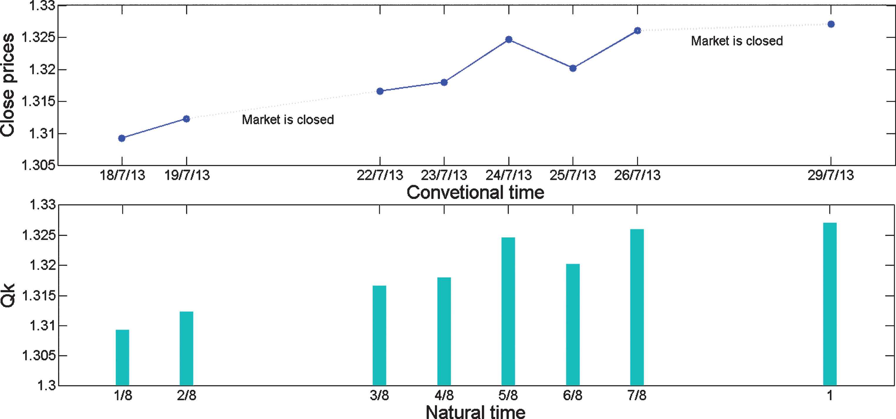
Fig.2
Upper figure shows one minute data of EUR/USD (date: 09/21/2012 from 07:50 until 18:07) in conventional time and the lower figure shows the evolution of variance κ1 (L=300) also in conventional time.
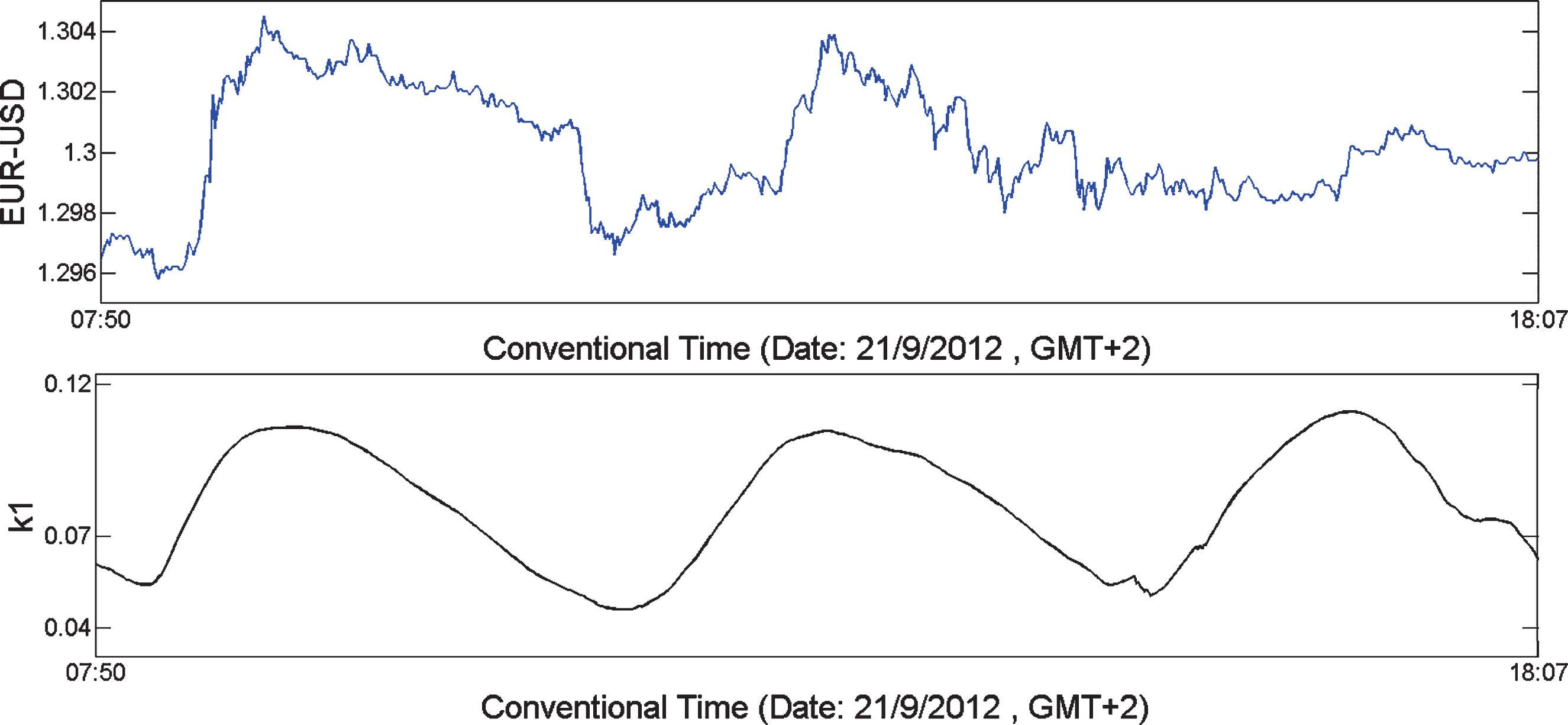
Fig.3
Upper figure shows one minute randomly shuffled data of EUR/USD (date: 09/21/2012 from 07:50 until 18:07) in conventional time and the lower figure shows the evolution of variance κ1 L=300) also in conventional time.
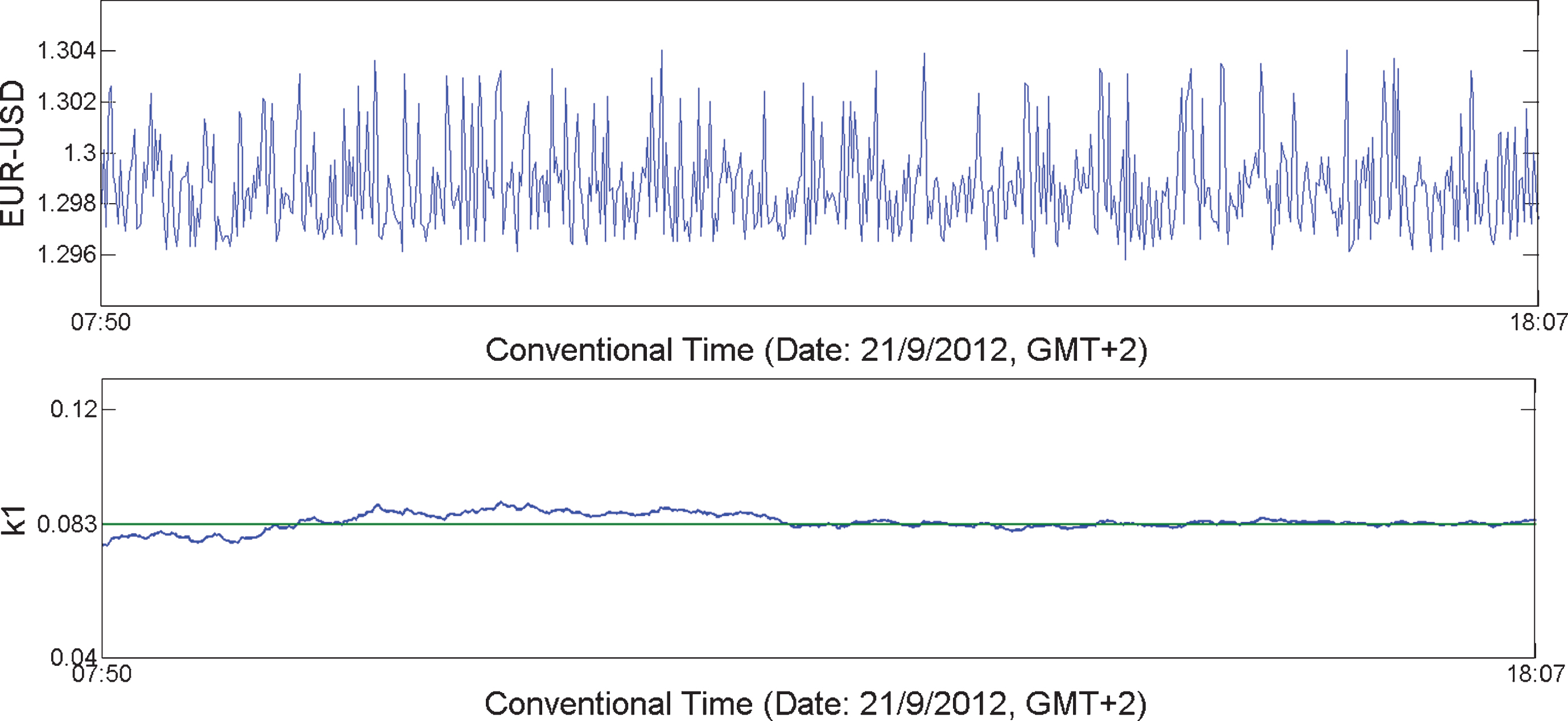
Fig.4
Upper figure shows one minute data of EUR/USD (date: 09/21/2012 from 07:50 until 18:07) in conventional time and lower figure shows the evolution of variance κ1 (L=300) also in conventional time. Green and red boxes show areas in the data of consecutive local extrema.
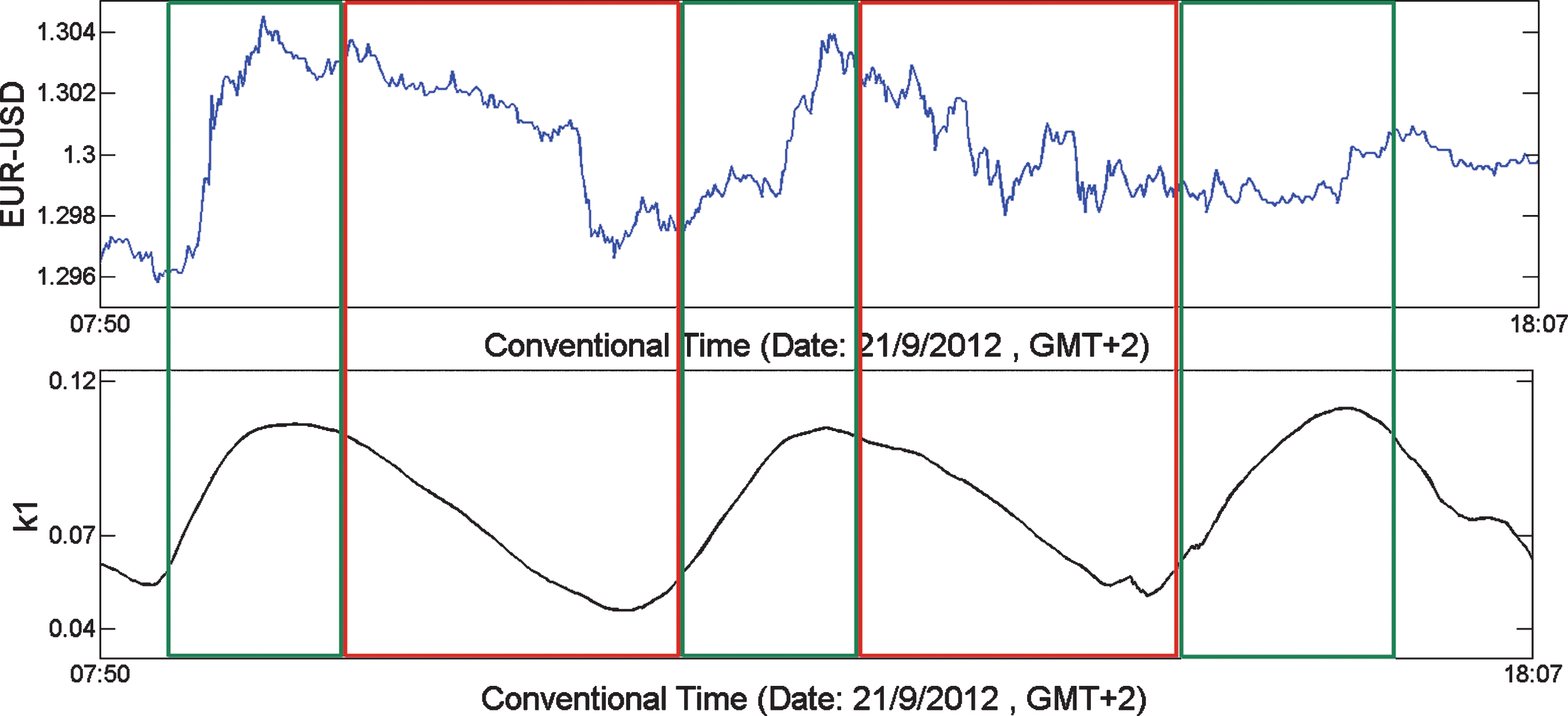
Fig.5
Upper figure shows one minute data of EUR/USD (date: 09/21/2012 from 07:50 until 18:07) in conventional time. Lower figure shows the evolution of variance of κ1 in different time windows (blue curve: larger time window (Lb = 300), green curve: smaller time window (Ls = 30)), also in conventional time.
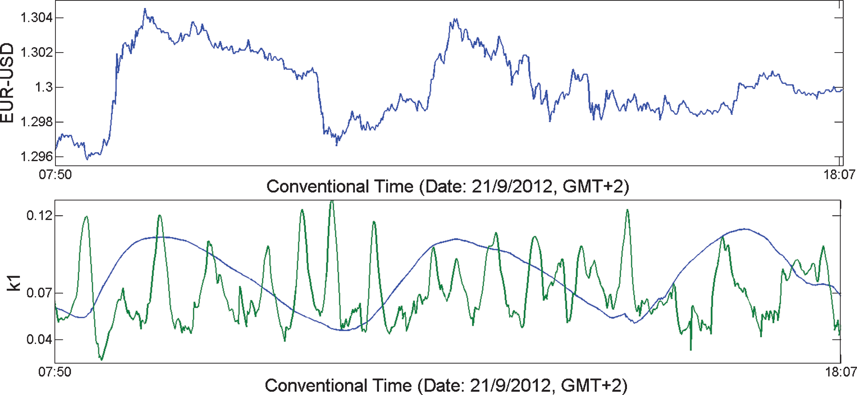
Table 1
Results for trading strategy based on Natural time analysis on major currency pairs (Trading Period: 1/1/2010 to 31/12/2013)
| Forex Returns | |||||
| Instrument | P&L | ||||
| 2010 | 2011 | 2012 | 2013 | 2010– 2013 | |
| AUD-USD | 13.80% | 7.67% | -4.03% | 4.65% | 22.09% |
| EUR-CHF | 13.26% | 8.97% | 3.18% | 0.70% | 26.10% |
| EUR-GBP | -0.36% | 5.90% | 3.18% | 11.83% | 20.55% |
| EUR-JPY | -0.26% | 6.29% | 15.41% | 20.82% | 42.26% |
| EUR-USD | 4.10% | -0.37% | -1.74% | 6.70% | 8.70% |
| GBP-USD | -0.96% | 5.90% | 1.41% | 11.83% | 18.17% |
| USD-CAD | 0.51% | 2.25% | -2.34% | 10.71% | 11.12% |
| USD-CHF | 6.39% | 26.27% | -1.09% | 19.62% | 51.19% |
| USD-JPY | 3.25% | 5.16% | 3.15% | 12.26% | 23.82% |
| AVERAGE | 4.42% | 7.56% | 1.90% | 11.01% | 24.89% |
Table 2
Results for trading strategy based on Natural time analysis on the 30 stocks of DJIA (Trading Period: 1/1/2011 to 31/12/2014)
| DJIA stocks’ returns | |||||
| Instrument | P&L | ||||
| 2011 | 2012 | 2013 | 2014 | 2010– 2014 | |
| AA | 78.7% | 14.6% | 47.0% | 38.9% | 179.2% |
| HPQ | 34.7% | 36.1% | 18.8% | -9.6% | 80.0% |
| BAC | 41.2% | 18.2% | 19.2% | -5.6% | 73.0% |
| MSFT | 10.4% | 17.0% | 28.7% | 16.9% | 72.9% |
| DD | 27.7% | 23.7% | -4.9% | 16.0% | 62.5% |
| UTX | 38.7% | 4.3% | 11.9% | 6.0% | 60.9% |
| BA | 37.3% | -16.5% | 18.2% | 12.8% | 51.9% |
| MRK | 18.4% | -14.5% | 17.5% | 18.5% | 39.9% |
| CVX | 0.3% | 8.0% | 23.2% | 4.2% | 35.7% |
| MMM | 15.1% | -7.5% | 24.1% | -4.2% | 27.5% |
| CAT | 20.9% | 18.1% | 21.2% | -33.6% | 26.6% |
| HD | -22.9% | 18.3% | 25.0% | 6.1% | 26.4% |
| INTC | 21.3% | -2.0% | 29.8% | -23.6% | 25.5% |
| IBM | 21.3% | 1.8% | -9.7% | 6.4% | 19.8% |
| T | -3.5% | 14.1% | 3.2% | 0.9% | 14.7% |
| PG | 23.4% | -8.4% | 0.1% | -7.4% | 7.7% |
| DIS | 24.0% | 0.4% | -11.2% | -5.7% | 7.4% |
| WMT | 0.2% | -1.4% | 2.1% | 2.4% | 3.3% |
| KFT | 0.7% | 0.5% | 0.9% | 1.1% | 3.2% |
| XOM | 15.2% | -12.8% | 1.5% | -1.2% | 2.7% |
| JNJ | 14.6% | -21.6% | 4.5% | 5.1% | 2.6% |
| VZ | 0.1% | 6.9% | -12.6% | 6.2% | 0.6% |
| AXP | -3.4% | 2.6% | 0.9% | 0.1% | 0.2% |
| JPM | 0.2% | -26.9% | -17.4% | 40.8% | -3.4% |
| GE | -0.4% | -12.2% | 1.3% | 3.2% | -8.1% |
| MCD | -18.8% | 14.2% | -5.0% | -1.7% | -11.4% |
| CSCO | 12.9% | 0.8% | -17.2% | -8.9% | -12.3% |
| PFE | -2.1% | -22.2% | -0.2% | 10.7% | -13.8% |
| KO | -5.4% | -2.2% | -11.7% | 2.1% | -17.3% |
| TRV | 12.3% | -27.4% | 4.3% | -10.2% | -21.0% |
| AVERAGE | 13.8% | 0.8% | 7.1% | 2.9% | 24.6% |
Table 3
Correlation coefficients of an equal weight portfolio with stocks of DJIA versus index returns and index volatility of DJIA
| Correlation Coefficients | ||
| Year | DJIA portfolio returns | DJIA portfolio returns |
| vs | vs | |
| DJIA volatility index | DJIA index returns | |
| 2011 | -0.65 | 0.27 |
| 2012 | -0.09 | -0.36 |
| 2013 | 0.10 | 0.35 |
| 2014 | 0.03 | 0.28 |
| 2011– 2014 | -0.35 | 0.25 |
| Calculated metrics based on monthly results | ||
Table 4
S & P500 portfolio based on Natural time Strategy
| Year | P&L | Sharpe | max | Value at | Expected | S&P 500 |
| Ratio | Drawdown | Risk | Value at risk | |||
| 2008 | 20.46% | 1.12 | -15.98% | -2.03% | -2.47% | -38.49% |
| 2009 | 25.22% | 2.21 | -6.53% | -1.06% | -1.86% | 23.45% |
| 2010 | 2.11% | 1.01 | -6.89% | -1.42% | -2.08% | 12.78% |
| 2011 | 17.81% | 1.92 | -6.36% | -1.33% | -2.04% | 0.00% |
| 2012 | 19.42% | 2.16 | -4.86% | -0.73% | -1.12% | 13.41% |
| 2013 | 19.85% | 2.28 | -3.49% | -0.62% | -0.77% | 29.60% |
| Calculated metrics based on Leverage 1:1 | ||||||
Table 5
Correlation coefficients of a portfolio constituting of 20 stocks of S & P500 versus returns of S & P500 index returns and versus S & P500 volatility index
| Correlation Coefficients | ||
| Year | S&P 500 portfolio returns | S&P 500 portfolio returns |
| vs | vs | |
| S&P 500 volatility index | S&P 500 index returns | |
| 2008 | 0.04 | 0.27 |
| 2009 | 0.01 | 0.21 |
| 2010 | 0.27 | - 0.11 |
| 2011 | -0.61 | 0.29 |
| 2012 | -0.19 | 0.17 |
| 2013 | 0.01 | -0.03 |
| 2008– 2013 | -0.03 | 0.18 |
| Calculated metrics based on monthly results | ||


