
Classifying falls using out-of-distribution detection in human activity recognition
Abstract
As the research community focuses on improving the reliability of deep learning, identifying out-of-distribution (OOD) data has become crucial. Detecting OOD inputs during test/prediction allows the model to account for discriminative features unknown to the model. This capability increases the model’s reliability since this model provides a class prediction solely at incoming data similar to the training one. Although OOD detection is well-established in computer vision, it is relatively unexplored in other areas, like time series-based human activity recognition (HAR). Since uncertainty has been a critical driver for OOD in vision-based models, the same component has proven effective in time-series applications.
In this work, we propose an ensemble-based temporal learning framework to address the OOD detection problem in HAR with time-series data. First, we define different types of OOD for HAR that arise from realistic scenarios. Then we apply our ensemble-based temporal learning framework incorporating uncertainty to detect OODs for the defined HAR workloads. This particular formulation also allows a novel approach to fall detection. We train our model on non-fall activities and detect falls as OOD. Our method shows state-of-the-art performance in a fall detection task using much lesser data. Furthermore, the ensemble framework outperformed the traditional deep-learning method (our baseline) on the OOD detection task across all the other chosen datasets.
1.Introduction
Many common applications rely on deep learning (DL) methods for Human Activity Recognition (HAR), such as providing feedback to athletes based on sensor data. HAR algorithms predict activities such as running, walking, or jogging to generate feedback. However, in these applications, the model often encounters out-of-distribution (OOD) activities, such as resting while running or answering a phone call, which it must differentiate from in-distribution (ID) data to avoid misclassification. Nevertheless, most state-of-the-art DL models used for HAR fail to do so. The primary reason is that these models are trained to discriminate between classes with high accuracy without considering the inherent uncertainty in the data and the model [17]. This inability of traditional neural networks to accommodate uncertainty compromises their robustness when encountering OOD data during test/production. Therefore, these models assert an equal confidence prediction for OOD and ID test data. As a result, the OODs are misclassified as IDs affecting model reliability and robustness. Therefore, uncertainty estimation is an essential task for detecting OODs. Unfortunately, OOD detection is an under-explored task in the wearable sensor-based HAR domain. Therefore, in this work, we try to empower traditional neural networks to detect OODs from time-series recordings of human activities. To properly evaluate the OOD detection capabilities, we propose OOD data exposing the HAR models to unforeseen discriminative features. In addition to that, we discuss how an ensemble-based temporal learning framework provides sufficient uncertainty to separate OODs from ID data in HAR tasks.
We begin by defining activity-based OOD examples. Since there can be a wide range of activities, we need to narrow the activities space so that the defined OODs possess distinguishable features to the training data. Hence we consider walking, running, jogging, standing, sitting, walking upstairs, and walking downstairs activities. Based on these activities, we define two categories of in-distribution (ID) versus out-of-distribution (OOD) examples, namely;
(1) Dynamic activities (ID) versus Static activities (OOD): In this set, the dynamic activities such as running, walking, etc. are used to train the model (ID) and the static activities such as standing, sitting are used as OOD. This type of OOD can be encountered in real life. E.g., static activities can be out-of-distribution in an athletic or sporting scenario where predictions are usually dynamic sporting activities. Detecting static OODs in those scenarios can help reduce the misclassification error of the model.
(2) Known activities (ID) versus Unknown activities (OOD): In this set, all but one activity are used to train the model, and the left out activity is used as OOD. This kind of scenario might occur in the real world, where we do not know about certain activities relevant to the HAR application. Detecting those activities as OODs allows discovering a new class that can be incorporated into the relevant activities.
To quantify the data uncertainty in this temporal setting, we have used a method from our previous work [31] called Deep time Ensembles (DTE). This method has two consecutive parts, i) extracting different temporal information by sliding window lengths of different sizes on the raw time-series input and ii) using that temporal information to train multiple models for ensembling. Initially, it was proposed to improve classification and calibration metrics for HAR tasks. Since calibration is a direct reflection of data uncertainty, in this work, we show that estimating uncertainty using DTE is also effective for OOD detection. However, traditional neural networks in HAR fail to detect OOD.
Traditional neural networks cannot internalize an entire recorded activity. Instead, they truncate the time-series recording to multiple temporal sequences extracted with the same window size. The fixed-size window will implicitly induce bias in the predictive response. In other words, the model is missing out on the data variability (uncertainty) since this requires a window size that corresponds to the designated activity’s entire duration. Compounding different predictive responses conveying incoherent biases induced by the different window sizes can enhance the data’s inherent (coherent) uncertainty. As a result, the prediction variance reflects the data uncertainty, and the incoherent biases are averaged out.
To attain coherent compounding within the DTE [31] setup, an ensemble of models is trained with sequences extracted with different window sizes. At inference time, the model’s predictive responses are averaged out. Different window sizes for extracting temporal sequence induces distinct bias in each model during training. Combining the predictive output from each model increases the uncertainty in data and reduces the uncertainty from the window sizes. This coherent compounding can also be explained through the lens of softmax function. Since the learning in DTE is distinct across models, so are their softmax outputs as well. Eventually, these distinct outputs, when combined, convey more uncertainty through a smoother softmax. In the case of ID data, a smoother softmax increases the values for incorrect classes predictions; nevertheless, it still reaches the necessary consensus for the correct class. However, this consensus does not hold for OOD data since the averaging would bring the class predictions close to a uniform distribution. This uniformity is a direct consequence of the harnessed data uncertainty by combining ensemble models. Hence, allowing it to estimate uncertainty in the OOD inputs with success.
This behavior can be visualized through the distribution of the predictive entropy (c.f Fig. 1). Since the training process reduces the entropy of the predictive response in the ID, the underlying assumption is that OOD samples maintain a higher entropy of their predictive distribution. In the case of ID data, the majority of the entropy coming out of the ensemble will be around zero, whereas the OOD data will push the entropy towards positive values.
Fig. 1.
Predictive entropy distribution for ID and OOD.
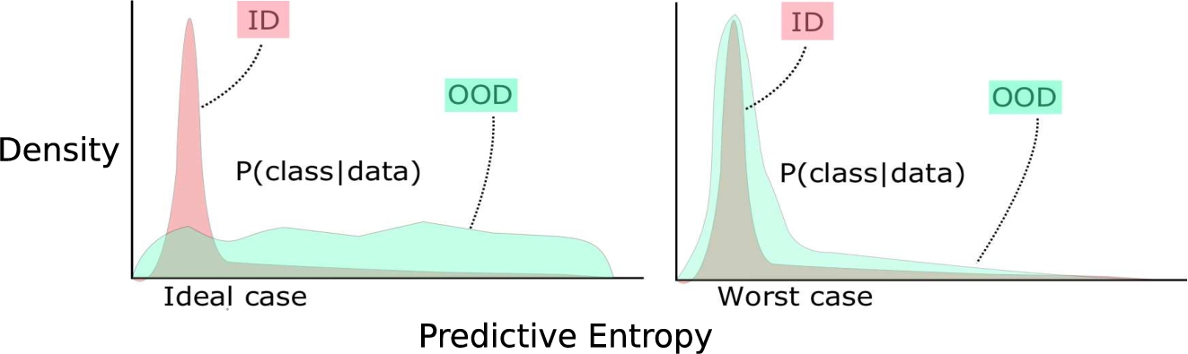
Estimating the density shift of the entropy distribution for OODs serves as the primary metric for their detection. This shift can be estimated by measuring the overlapping area under the curve between ID and OOD entropy distribution. Therefore, Weitzman’s Measure [7] calculating the overlapping area under two functions could serve as an elegant metric for the density shift. The lower the intersection area, the better the OOD detection for the model and vice-versa. This metric serves better than traditional divergence-based metrics that compare two different distributions. Divergence-based methods are harder to compute and can possess numerical problems when the modality of two distributions is not equal. In contrast, the Weitzman’s Measure would be able to quickly tell that there is a noticeable overlap between these distributions and hence will provide the correct OOD score.
Deep time-ensemble [31] is tested on defined OODs extracted from three popular sensor-based HAR datasets, WISDM [36], UCI [3] and Motion-Sense [25]. It outperforms the baseline model [24] (a CNN architecture adopted from previous work) on the OOD detection tasks on the introduced metrics for the chosen datasets.
This paper is an extension of a previous paper published at a workshop. The main contribution of this paper is defining simple and effective OODs for HAR with wearable time-series data and using our previous ensemble-based temporal framework to detect them. We also provide reasoning to explain why DTE suits OOD detection tasks with temporal workloads. While a few works address uncertainty estimation in HAR, to the best of our knowledge, none of them address the OOD detection paradigm. In addition to the existing content, we have extended the paper by showcasing how the OOD detection method can be used in a use-case of elderly fall classification. In particular, it can reduce the amount of data substantially by training models only on the non-fall activities and detecting the falls as OODs.
The paper is organized as follows: Section 2 discusses the Related Work. Following this, the Methods argues the rationale behind using DTE for OOD detection. The initial Experiment and Results are presented in Section 4, followed by a Discussion and, Conclusion and Future Works section.
2.Related works
Three categories of work are discussed in this section: The first one discusses the works in general activity recognition, their evolution, and where this article resides in that paradigm. The second group discusses uncertainty estimation methods in deep-learning and compares how the method used in this paper is different. The third group reviews an intersection of both the above groups and compares this work with its closest alternatives. Finally, the fourth class of related work reviews on anomaly detection in the context of time-series IoT environments.
2.1.On activity recognition
Activity recognition (AR) with wearable sensors [5,36] is popularly achieved using deep learning methods [11,14,23,30,35]. Popular choices of deep-learning architectures include CNN based on 1D convolution of time-series data [14], recurrent neural-networks [28], autoencoder-based architectures [34]. However, these methods produce classification estimates without addressing data or model uncertainty. Hence, they react inefficiently with concept drift in the dataset and fail on the OOD detection task. Deep time-ensemble method [31], used in this paper, can adapt to any deep-learning architecture and detect OOD successfully.
2.2.On uncertainty estimation
Estimating uncertainty in neural networks makes them more robust and helps detect possible domain-shift in the data. From a probabilistic viewpoint uncertainty aware neural networks can be classified into Bayesian [6,9,18] and, Frequentist [21,33]. A popular application of Bayesian formalization in neural networks is to learn a probability distribution of the neural network weights that helps in uncertainty estimation [6]. However, the complexity of training a Bayesian neural network (for many applications) and complex prior assumptions motivated the researchers to explore probabilistic estimation using standard neural networks. Ensemble-based methods have generated much traction in recent years due to their ability to estimate uncertainty while utilizing standard neural network architectures [21,24,26]. Vyas et al. [33] formulated a loss function that, when added to standard cross-entropy loss of a neural network, increases the margin of separation between ID and OOD samples of images. They train an ensemble of neural networks in a self-supervised fashion with this composite loss function. Lakshminarayanan et al. [21] establish that through ensembling and adversarial training, deterministic neural networks can be enforced to estimate uncertainty. They show success in examples from computer-vision and standard regression datasets.
However, the ensembling method proposed in our earlier paper is designed to adapt time-series workloads that were not explored in [21,33]. Other works that addressed OOD detection explicitly are [12,22,24]. A work by Hendrycks et al. [12] showcases that although viewing softmax output in isolation can be misleading in identifying OOD, and ID samples, collecting the global statistics about the softmax of ID samples can help differentiate ID and OOD samples. Lee et al. [22] separate OOD and ID by training a GAN network, with cross-entropy loss and a loss term based on distance from a uniform distribution. Liang et al. [24] increased the margin between ID and OOD samples by having temperature scaled softmax outputs into the cross-entropy loss and small perturbations in the training example.
Recently transformer-based models have been used in quantifying uncertainty. Large-scale transformer-based models have been successfully used to push the state-of-the-art OOD detection in computer vision tasks [8,20]. Pre-trained transformers and contrastive learning combined together have also shown successful OOD detection capabilities [38]. Transformer-based solutions to detect OOD have also been applied to a practical clinical use case to segment hemorrhage in head CT-scans [10]. Transformers are very powerful and have proven to be immensely successful in many scenarios of OOD detection, but large-scale transformers are computationally expensive.
Most of these methods discussed for uncertainty estimation and OOD detection have been extensively tested and benchmarked on computer vision problems and regression tasks. However, they are a bit under-explored in the context of time-series data, particularly HAR. This paper leverages the ensemble-based uncertainty estimation concept and demonstrates its capability for sensory recordings of time-series data on HAR tasks.
2.3.A combination of both
While activity recognition is a well-established field, with uncertainty estimation in deep learning not far behind, the combination of both is relatively new. While Nweke et al. [29] researched the usage of sensor-level ensemble stacking and improved misclassification in HAR, they did not investigate the impact of OOD on their models. Hue et al. [13] explore annotation uncertainty and mitigate the issue by a soft-labeling strategy. They tackle an uncertainty problem in activity recognition with RGB-D frames. It is comparatively more manageable for the annotator to assign soft labels to ambiguous activities with visual aid. Hence the model gets more labelling assistance for uncertainty estimation. On the other hand, deep time-ensemble [31] deals strictly with wearable-sensor-based activity recognition, where it is more complicated to annotate ambiguous labels from sensor data. Akbar et al. [1,2] approaches uncertainty in activity recognition with generative modelling. Akbar et al. [2] propose a method that allows easy integration of new sensor data with models trained with the older sensor data. The closest match to this work is with [1], where the authors propose a Bayesian CNN as a variational autoencoder [19] for estimating the density of sensor signals. Later they use the estimated density to sample and classify activities as a downstream task with a classification layer and Monte-Carlo dropout [9]. While it is an elegant way to estimate uncertainty, the authors [1] do not explicitly explore the OOD detection ability. The used deep time-ensemble [31] is potentially more straightforward (because of the non-Bayesian approach) and is used for detecting OODs in HAR tasks.
2.4.On anomaly detection
Anomaly detection with machine learning is a problem where the models try to identify anomalous classes, i.e. classes that are outliers with respect to the classes the model has been trained on. Intuitively, out-of-distribution data on other hand might be an outlier class or simply a new class that has not been encountered before. The requirement of an ood class (outlier or not) must be that it will be drawn from a distribution that is statistically different from the training data distribution. While there is not a strict separation between the two, in our understanding anomaly detection is a stricter variant of out-of-distribution detection. Some applications of ood detection might deal with outlier classes and hence it is important to look at the existing state-of-the-art in anomaly detection.
In particular, anomaly detection using machine learning has garnered enough attention in the domain of IoT and smart-home [4]. Mining time-series stream data [15], user-behavior [16] has provided security solutions. Detecting medical events [37] is also another important use-case in sensor-driven anomaly detection problems. However, most of the existing anomaly detection techniques using machine learning demand exposure to a few examples of anomalous data. This might be restrictive in a certain context. Using our proposed out-of-distribution (OOD) in the anomaly detection task, we can bypass the requirement to have some anomalous training data (see Section 4) for more insights on this.
3.Methods
3.1.Integrity of uncertainty in deep learning
Harvesting the necessary uncertainty presented in the data has proven beneficiary in increasing the awareness of a machine learning model toward OOD test data. In a deep learning classifier, usually, the softmax layer accommodates some stochastic behaviour of the data. The rest of the layers are dedicated to generalizing the representative features. On the one hand, the high number of such components (layers) makes a classifier more capable of achieving high predictive accuracy. On the other hand, the single last layer consolidates uncertainty from the data to a much lesser extent than needed. Based on the bias-variance trade-off, the more uncertainty incorporated in the model, the lesser unwanted bias in the final prediction. Thus, stochasticity must be included in the layers before the softmax to make the model less deterministic. An ensemble is a popular approach for delivering such behaviour. The multiple models in the ensemble simulate the behaviour of such stochastic layers.
3.2.Problem setup
A temporal sequence X is obtained by sliding a particular window size over the raw time-series data. The goal is to predict the activity based on the observations defined by X. This temporal sequence X is fed to a neural network
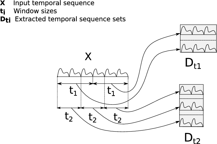
Temporal sequence, X, can be re-represented as a combination of multiple temporal sequences extracted with different window sizes. As shown in Fig. 2, X is represented as temporal sequence sets
Fig. 2.
Representing a temporal-sequence X as a collection of different temporal sequences by using different window-sizes.
3.3.Deep time ensembles for uncertainty estimation
Time series recordings have the structural information encoded into their temporal order. Namely, whenever a particular trend is present in a time series, it will persist throughout consecutive recorded values. The data fed into the model is strictly ordered by the acquisition time. The scope of exploration depends explicitly on the number of consecutive values fed into the model. Traditionally, in activity recognition problems, this is achieved by extracting data (a temporal sequence) using a fixed window size and feeding it to the model. Thus, extracting the temporal information is highly dependent on the window size of sensor readings. A naive ensembling technique that trains multiple models using identical temporal sequences obtained by using the same window size is sub-optimal. The equation of output from such ensemble is given by Eqn (1). Having the same window size would extract the same temporal sequence X, that is fed to the M models in the ensemble. It conveys the same information to each model in the ensemble. The only source of randomness, in this case, is obtained through converged weight values
On top of the softmax averaging, in the combination step of ensembling, DTE also features nested averaging. This is evident from Fig. 2. When temporal sequence X is represented as a collection of temporal-sequences
3.4.Density of entropies
The coherent uncertainty of the model is mainly a consequence of the incompatible prior assumption made for the model. This type of uncertainty persists through the training process for the given data. The incoherent uncertainty of the model is then a direct consequence of the imperfect calibration of the hyperparameter of the model. This type of uncertainty is generally misleading as it is just a subjective reflection of the hyperparameters and clutters the coherent uncertainty. An ensemble can suppress the incoherent uncertainty, eventually decluttering the model uncertainty. The predictive output comes as a normalized distribution degree of belief, also known as softmax output (cf. Eqn (3)).
The overall uncertainty represented by the softmax is then compressed into a single empirical value using entropy. The entropy weights the softmax output by the amount of information that a particular output possesses (cf. Eqn (4)). The more uniform the predictive output is, the more uncertain the model is, resulting in a higher entropy value.
Using a collection of entropies that fully characterizes the ensemble represents the total amount of uncertainty produced by the model for a given test data. The model is highly confident whenever entropies are close to zero, and the uncertainty is relatively low. These cases are mostly related to ID data, where the model has been heavily trained. Whenever there are OOD data, the ensemble produces a frequent amount of high entropy values, given that predictive outputs are, on average, distributed at equal probabilities. Furthermore, having a density estimation from the collection of entropy values is then computationally attractive to judge the overall behaviour in an ensemble.
3.5.Density-shift estimation
The final output of an ensemble is a distribution of entropy values, and assessing the discrepancy between two different distributions in the context of density shift is not as trivial. OOD distribution entropies are expected to shift their density mass towards high positive values, whereas ID entropies remain around zero. A measure that fits the need the most should target the density shift and put lower importance on the shape of distributions. Weitzman measure (cf. Eqn (5)) quantifies this shift quite elegantly by measuring the amount of intersecting area between two distributions. The farther apart from one another two distributions are, the lower the Weitzman measure (wm) is and the better the OOD detection capability of the model.
4.Elderly fall detection – an use-case of OOD detection
Fig. 3.
Fall detection usecase.
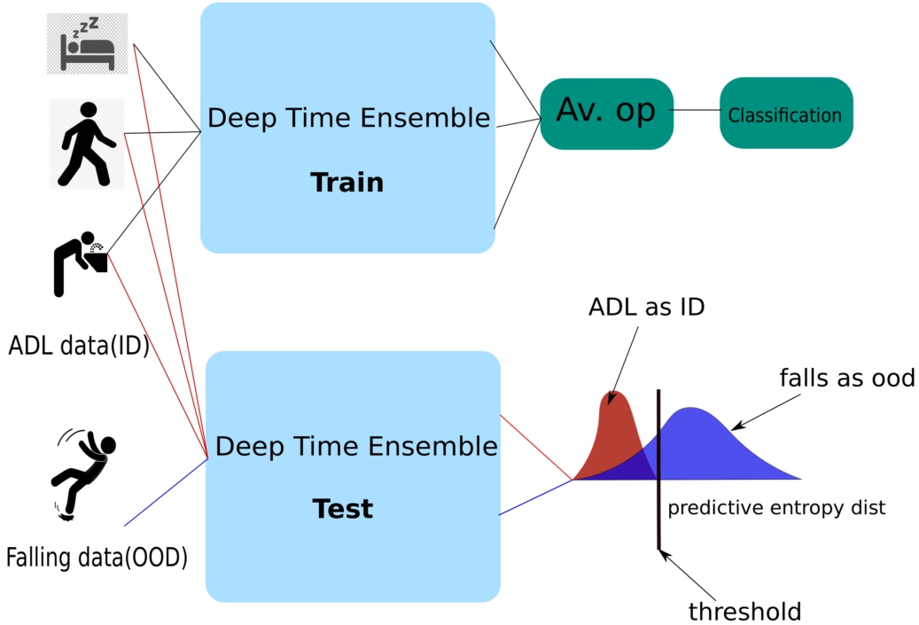
Elderly fall detection being a vital application in geriatric care is a use-case where the application of Deep time-ensemble showed promising outcomes with lesser data. The traditional fall detection task involves training DL models on ADL activities along and simulated/real falls. The problem with this approach is that to detect falls reliably, the model needs to learn the fall patterns from the training dataset. This calls for an extensive and well-curated fall dataset with examples of all the different types of falls. The highly stochastic nature of the falling down activity and the corresponding wearable signal pattern it can produce makes this problematic, inspiring exploration of alternative directions.
Based on the primary proposition of this paper, a new fall detection system is proposed where the falls are detected as OOD. The process is explained in Fig. 3. The proposed system is trained only with non-fall activities from a standard fall dataset using the Deep time-ensemble method. Thus when probed with Falling samples, it produces a higher predictive entropy at the output, detecting it as a fall. Since predictive entropy is derived from the probabilistic softmax output, the softmax output can be used to separate OOD from ID. The confidence estimate of the prediction, that is, the maximum value of the softmax output, is used for the same purpose. A threshold can be drawn based on the confidence of the predictions from the model that mark samples below the threshold as probable falls. Not only this system allows to raise alarms and have a human-in-the-loop scenario for emergency geriatric care services but also it drastically reduces the amount of training data required to train a fall detection system.
5.Experiment and results
We have used a CNN architecture adapted from Ignatov et al. [14] as the baseline model and ensembled the same architecture using DTE. Since, DTE [31] also compared with Ignatov et al. [14] using the same CNN architecture, the configurations of the window-sizes and hyper-parameters were directly adopted from [31]. The goal of the experiments was to detect OODs extracted from standard HAR datasets. For classification results, we would refer to our previous work [31].
5.1.Datasets
We have primarily defined OODs based on activities from WISDM [36], UCI [3] and Motion-Sense [25] dataset. Below we discuss the datasets and how they are used to formulate ID and OOD data.
5.1.1.WISDM dataset:
The WISDM dataset consists of accelerometer recordings from six activities, namely, walking, jogging, upstairs, downstairs, sitting, standing obtained from 36 subjects. The baseline model is trained on 200 timesteps indicating 10 seconds of time-series data [14,31]. The DTE is trained on time-steps ranging from 200 to 100 [31]. The WISDM dataset is divided based on the activities. Dynamic activities walking, jogging, upstairs, downstairs form the Dynamic WISDM dataset, and static activities, i.e. sitting and standing forms the Static WISDM. Dynamic WISDM is used for training the models. Static WISDM is used as an OOD set.
5.1.2.UCI dataset:
The UCI dataset consists of 6 activities lying, standing, sitting, downstairs, upstairs, and walking recorded from 30 subjects. The modality of the sensor is a triaxial accelerometer and gyroscope resulting in 6 dimensions. It is used as ID data for our experiments. The baseline model is trained on 256 steps of UCI dataset ([14,31]. DTE trains 5 models between the range of 128 to 256 timesteps [31].
5.1.3.Motion-sense OOD dataset:
This dataset [25] consists of accelerometer and gyroscope readings from six activities, downstairs, upstairs, sitting, standing, jogging, walking. Since the UCI dataset does not have an instance of jogging, the input signal(accelerometer and gyroscope) for jogging is used as an OOD input to the models trained on the UCI dataset.
5.1.4.Sisfall dataset:
For our fall detection use case, we have chosen the Sisfall [32] dataset. The dataset is recorded using smartphones and consists of a triaxial accelerometer, gyroscope, and magnetometer recordings. 19 activities of daily life (ADLs) and 15 fall types were recorded in a simulated environment among young adults and elderly people. Like most fall detection systems, our goal was to classify falls from ADLs. Since our method did not require any fall data during the training procedure, we trained models only on the ADLs. The falls were used as OOD data inputs to the models.
5.2.Uncertainty estimation: OOD vs ID inputs
Based on the definitions of OOD in the Introduction, two experiments were formulated.
Dynamic WISDM as training and Static WISDM as OOD.
Training on full UCI dataset and using jogging from Motion-Sense dataset as OOD.
The predictive entropy distribution of the output is a central concept for visualizing uncertainty estimation in classification tasks. When tested with OOD examples, a well-behaved model provides uncertain or low-confidence outputs. This essentially translates to higher predictive entropy for the outputs. However, for the ID samples, the confidence is higher, and hence predictive entropy of the output is lower. Thus an ideal model gives low predictive entropy for ID samples and higher predictive entropy for OOD samples. In terms of Weitzman measure used to evaluate the model, a lower score indicates better OOD detection.
The hyperparameters and model architecture are presented in the Appendix. Next, we discuss the results of the experiments.
5.2.1.Probing dynamic WISDM dataset with OODs:
The models trained on Dynamic WISDM dataset are probed with Static WISDM dataset as OOD. For the baseline model, the predictive entropy distribution resides in a low-value region with a mean around 0 for both ID and OOD sets Fig. 4. DTE reacts similarly for the ID test data. However, for the OOD, i.e., static data, the predictive entropy distribution of the outputs shifts further to the right. The clear margin of separation in entropy distribution between ID and OOD data for DTE reflects in the Weitzman measure metric as well. The Weitzman measure is 2.3 times lower for the Deep time-ensemble compared to the baseline model.
5.2.2.Probing UCI dataset with OODs:
The expected behaviour is well-captured in the experiments, as showcased by Fig. 5. The ID test inputs to the baseline model produce low entropy values as expected. However, even for OOD datasets(Gaussian and Motion-sense OOD), the predictive entropy resides in the low-value region. It signifies overconfident misclassified outputs by the baseline.
DTE, on the other hand, produces high entropy values for OOD inputs and low-entropy values for the ID inputs. There exist a clear margin of separation between the ID and OOD datasets for DTE trained models. The above result is also quantified by the Weitzman measure, as shown in Table 1. The Weitzman measure shows a 4-fold decrease for the DTE compared to the baseline, for Gaussian OOD and 2.5 fold decrease for Motion-sense OOD dataset. Lower Weitzman measure indicates lesser overlap between ID and OOD samples and hence a better margin of separation.
Fig. 4.
Comparing OOD detection of a single model against Deep time ensembles. The training dataset consist of dynamic activities from WISDM, and the OODs are the static activities.
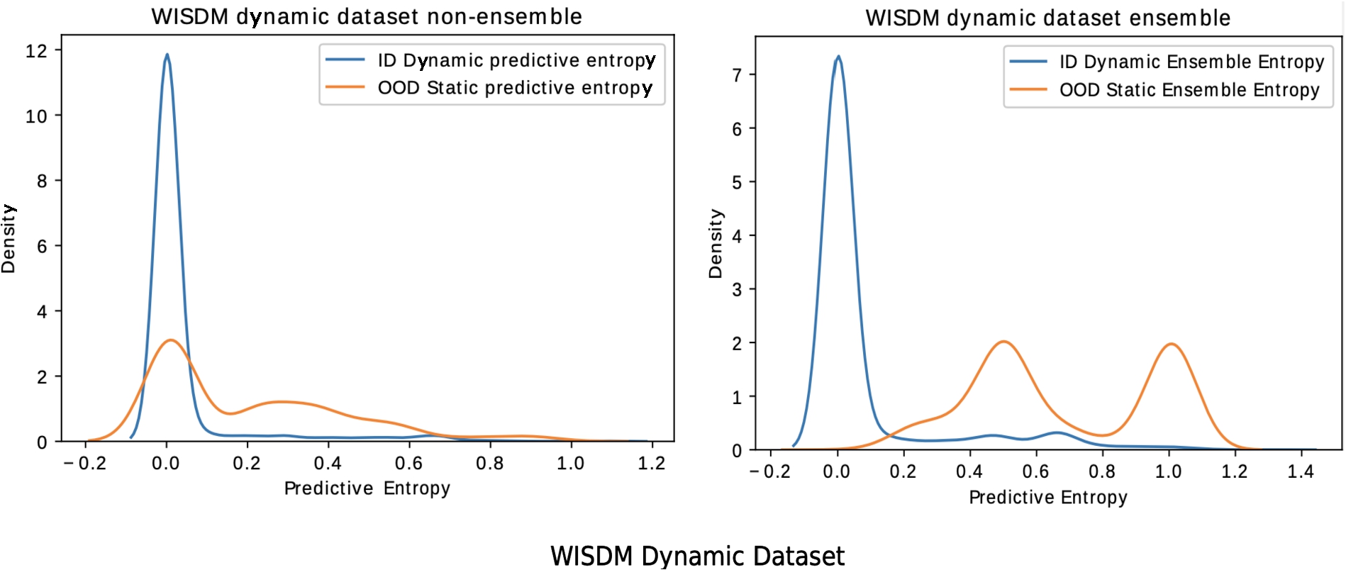
Fig. 5.
Comparing OOD detection of a single model against Deep time ensembles. The training dataset consists of dynamic activities from UCI, and the OOD is Jogging from the Motion-Sense dataset (other OOD in image) and random Gaussian noise.
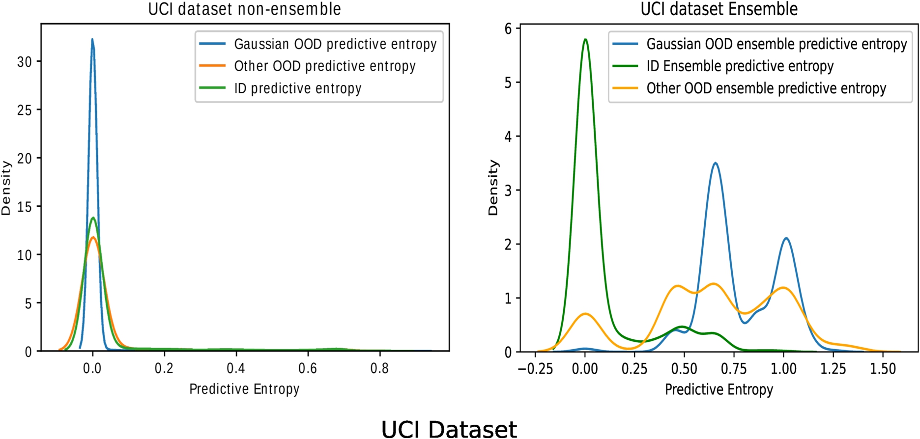
Table 1
Weitzman measure for different types of OOD – UCI dataset
| Model-type | Gaussian-OOD | Motion-sense OOD |
| Ensemble | 0.10 | 0.29 |
| Non-ensemble | 0.43 | 0.82 |
5.3.Results on elderly fall detection
For proving the effectivity of the method in the Fall Detection use case, we have chosen the Sisfall dataset. In our previous paper, we partially used the Sisfall dataset and showed that it could successfully detect falls as OOD. In Fig. 6, we show the density of predictive entropy for three cases:
(1) Out-of-distribution data, i.e., falls on Deep Ensembles.
(2) Out-of-distribution data, i.e., falls on the best-performing single model.
(3) In-distribution data, i.e., ADLs on Deep ensembles.
We also observe that deep ensembles have a reasonable margin of separation between ID and OOD data in predictive entropy. The overlap is more for the deterministic model, which makes it harder to separate ID and IID. The Weitzman measure for both ensembles and non-ensembles is presented in Table 2.
Fig. 6.
Predictive entropy fall detection use-case.
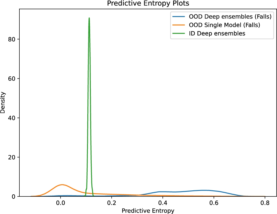
Table 2
Weitzman measure for falls as OOD – Sisfall dataset
| Model-type | Fall-detection-OOD |
| Ensemble | 0.08 |
| Non-ensemble | 0.2 |
Fig. 7.
Predictive confidence fall detection use-case.
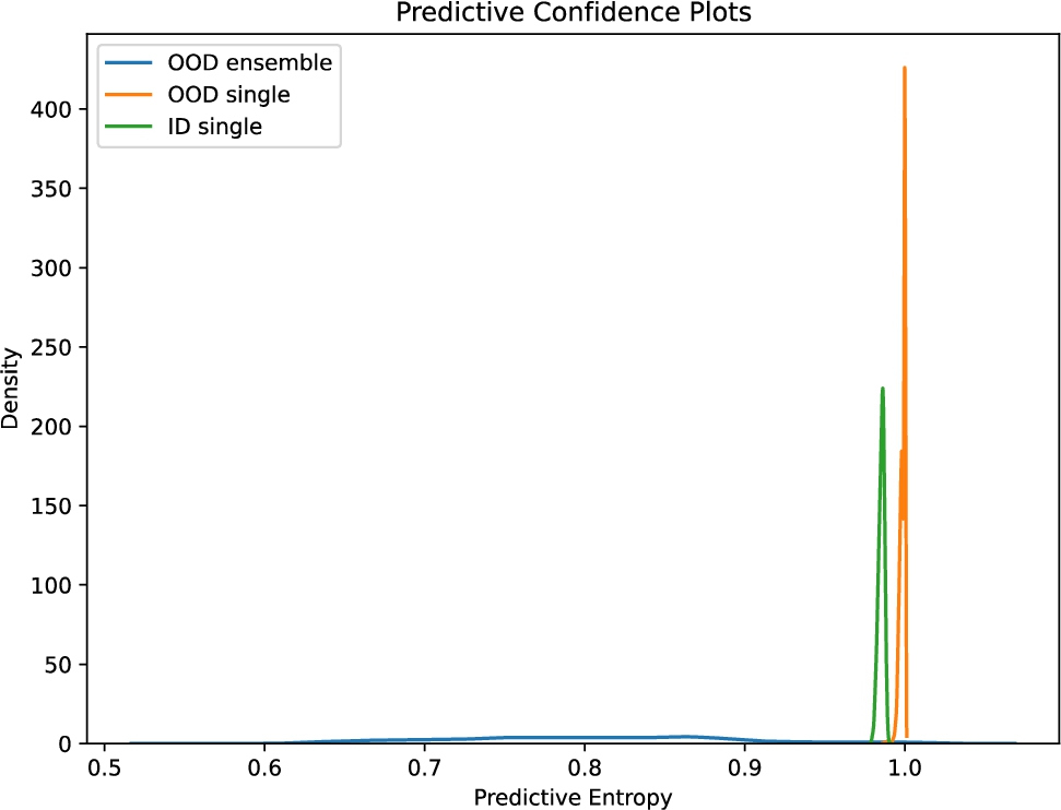
In general, we rely on the predictive entropy of the output to visually interpret OODs from IDs. In this case, using predictive confidence as a proxy of OOD detection allows us to draw a threshold to classify OODs from IDs. The predictive confidence of the prediction curve is provided in Fig. 7. This curve is the opposite of the predictive entropy curve. As seen, the ensemble model exhibit lower confidence for OOD data than ID data. On the contrary, the single deterministic model exhibits high confidence for both ID and OOD. This figure helps us decide on a threshold between the ID and OOD based on the confidence of the output. When using the ensemble model (i.e., Fig. 7) we can safely deduce that any predictions having a confidence value of 0.9 will be an ID, and the rest will be OOD. If we use the deterministic model instead, it will be harder to do so because it misclassifies the OOD outputs with high confidence.
Detecting falls as OOD in our threshold method allows the detection of almost 98 % of the falls successfully. Furthermore, since we do not use the falls in the classification training, it reduces the data load for training substantially, resulting in faster training.
6.Discussion
6.1.On OOD detection
A couple of interesting observations can be made from the experiments.
Firstly, it is clear from the Weitzman measure of different experiments that the random Gaussian noise is more out-of-distribution compared to the real datasets (see Fig. 9). This behavior is expected because the random Gaussian noise was deliberately drawn away from the training distribution. It served as a first step to show that DTE could pull apart the Gaussian noise successfully as OOD from the ID samples. However, the single model failed to do so even though the Gaussian noise values do not contain any discriminative features that the model is trained on. As a result, the single model misclassified the random data and assigned a high score to one of the classes in the softmax output. In DTE, however, even though individual models assign a high score (in softmax) to one of the classes, not all assign a high score to the same class. Thus, through averaging, the overall softmax output of the ensemble is smoothed to be more uniform. This uniformity translates to a higher entropy value for the predictive response, differentiating the OOD from ID.
When jogging activity from Motion-sense dataset is used as an OOD, there is a small overlap in predictive entropy distribution even for DTE (see Fig. 5). The similarity of jogging with some ID activities such as running and walking might be why. The discriminative features extracted by each model in DTE are not sophisticated enough to differentiate between jogging and some of the ID activities. There is a consensus among the models on the predicted class for some OOD data. Hence low uncertainty is obtained through model averaging. Thus, some portion of the realistic OOD dataset may be detected as ID, which explains the overlap. One possible way to mitigate this is by adding more layers to each model for improved feature extraction for each class. However, the models risk overfitting in the classification task. Since DTE is also optimized to obtain better predictions, overfitting each model would oppose that.
All the images (Fig. 4 and Fig. 5) with DTE shows an interesting feature. There is a bump in the predictive entropy distribution on the right-hand side, even for ID samples. Since each model in DTE produces a distinct output, there are some cases where the uncertainty in ID data does not allow for a consensus for the majority class in the softmax output. In those cases, the randomness of the model increases during the averaging process. Intuitively, these can be some borderline examples of ID data corrupted by noise or incorrect annotation.
The Weitzman measure calculates the overlapping area under the curve of the predictive entropy distributions between ID and OOD examples. This metric varies substantially among the different datasets presented. This is observed when comparing the Sisfall dataset with the other cases. For e.g., the Weitzman measure values in Table 2 are 0.08 (ensemble case) and 0.2 (non-ensemble case), whereas, for other datasets, the value of the ensemble case is usually between 0.1 to 0.3 (see Tables 1 and 3). This phenomenon can be attributed to the fact that in the Sisfall dataset, the in-distribution predictive entropy curve is almost a Gaussian with the least variance (Fig. 6). Since the goal of the Sisfall dataset was to classify falls, the in-distribution classification task was simplified by joining similar activity groups. This led to a higher classification accuracy compared to the other datasets and hence a sharper ID predictive entropy peak. This ensures that the overlapping area with the predictive entropy of the OOD samples (both non-ensemble and ensemble) is sufficiently lower compared to other datasets (WISDM and UCI). Thus, in this case, even the non-ensemble model has a Weitzman score closer to the ensemble variants for the other datasets. When using deep ensembles, we also observe that the OOD predictive entropy curve for the Sisfall dataset lies the furthest, indicating that this dataset has the easiest separation of OOD samples.
(1) Single deep learning models for the HAR tasks produce misclassifications in the face of OOD data because of their inability to capture uncertainty. This property may guide users towards wrong interpretations and make the models unreliable.
(2) Deep time-ensemble can estimate the uncertainty associated with the OOD samples and establish a clear margin of separation. A property desired for robustness and reliability.
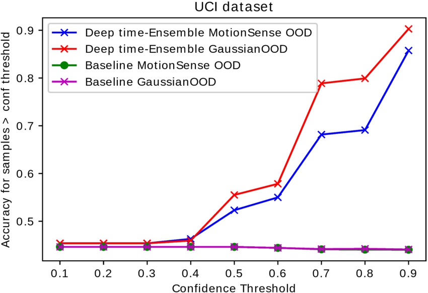
6.2.Accuracy vs confidence
One way of analyzing the uncertainty estimation ability of a model is by looking at the accuracy vs. confidence curve. Given a model prediction
Table 3
Weitzman measure for different types of OOD – WISDM dynamic
| Model-type | WISDM static OOD |
| Ensemble | 0.16 |
| Non-ensemble | 0.38 |
Fig. 8.
Confidence versus accuracy curve: comparison among baseline model and DTE on WISDM dataset. OOD in this experiment is static WISDM.
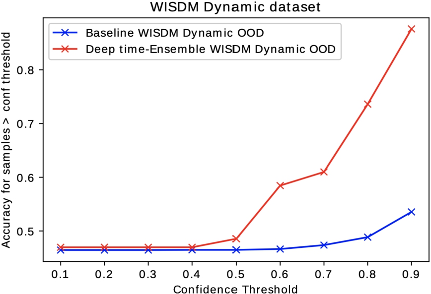
Fig. 9.
Confidence versus accuracy curve: comparison among baseline model and DTE on UCI dataset. OOD in this experiment is Jogging from Motion-Sense and random Gaussian noise.
7.Conclusion and future work
In this work, we set out to define and detect simple yet effective out-of-distribution (OOD) data for Human Activity Recognition (HAR) tasks. In particular, HAR problems with time-series data originating from wearable sensors. The defined OODs are usually encountered in realistic scenarios where HAR models are deployed. Although OOD detection is explored in the domain of computer vision and specific regression tasks, to the best of our knowledge, no previous work defines OODs for time-series workloads originating in the HAR domain. To detect the proposed OODs, we have adopted an ensemble-based framework called Deep Time Ensembles (DTE) that considers the workload’s temporality. In particular, we have used a baseline convolutional neural architecture that yielded promising results in HAR tasks from [14] and ensembled it using DTE. Our experiments on OOD data extracted from popular HAR datasets indicate that DTE outperforms the baseline model in detecting OODs. This nature will allow DTE to be incorporated for modeling robust and reliable solutions in HAR. It opens up exciting research avenues to be explored in the future, e.g., incorporating OOD detection with DTE in safety-critical HAR applications. One such application, Elderly Fall Detection, is presented in this paper. In our use case with Fall Detection, we tried to show how uncertainty estimation could detect falls with less data. Our results on the Sisfall dataset validate our idea and pave the path for future research.
While this work delves into some initial and simple OOD definitions for the HAR task, more interesting OODs for time-series data could be defined. E.g., In-distribution (ID) data originating from periodic activities versus OOD originating from aperiodic activities. Also, using OOD metrics to measure uncertainty arising from IoT devices could lead to better fine-tuning and calibration. Although ensembling captures stochasticity, the inherent complexity of training an ensemble can still be an issue. However, progress in distilling the ensemble models [26] is a direction that could be explored for the sensor data domain. Apart from extensive testing on more fall detection datasets, OOD detection, and the proposed metrics can find applicability in other domains such as sports, mobile sensing, etc., where time-series data from sensors play a vital role. The research presented in the paper defines interesting OODs and successfully demonstrates that OOD detection can be used for HAR tasks with a simple yet effective method.
Acknowledgements
This project has received funding from the European Union’s Horizon 2020 research and innovation programme under the Marie Skłodowska-Curie grant agreement No 813162. The content of this paper reflects the views only of their author (s). The European Commission/Research Executive Agency are not responsible for any use that may be made of the information it contains.
Appendices
Appendix
AppendixConvolution architecture and implementation details
In this section we present the convolution architecture in Fig. 10 and the model hyper-parameters in Table 4.
Fig. 10.
Convolution architecture used for modelling baseline and DTE.
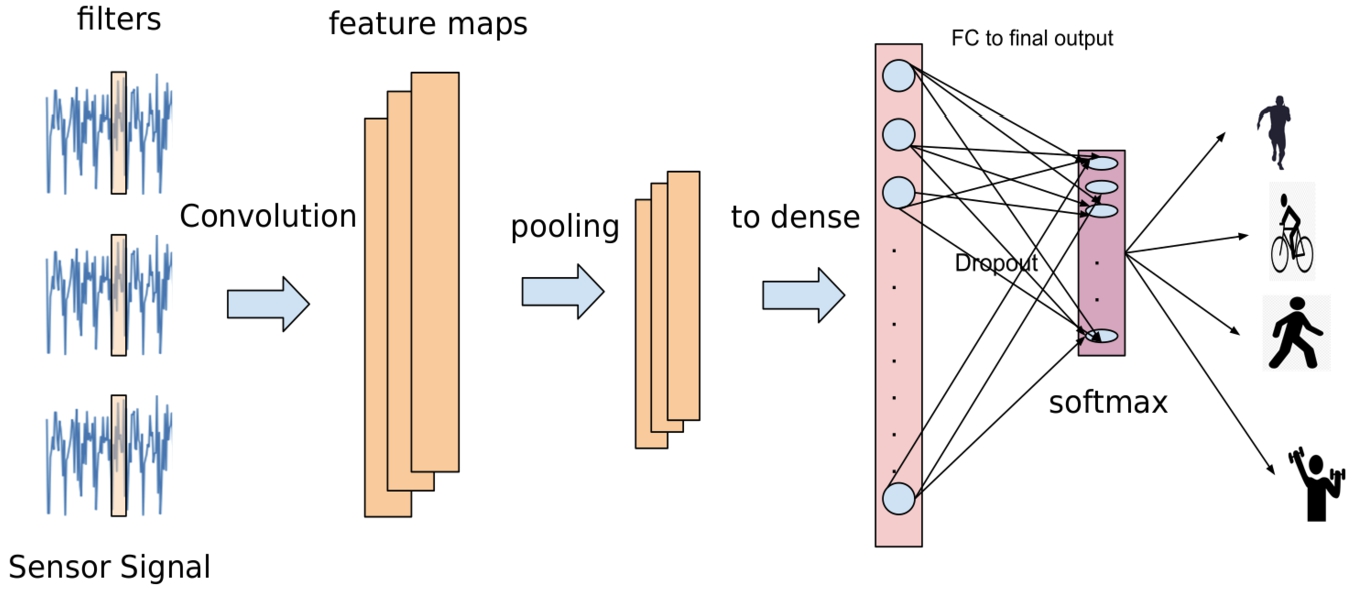
Table 4
Implementational details for results
| Datasets | UCI | WISDM |
| Ensemble size | 6 | 6 |
| Timesteps | [128, 100, 80, 70, 60, 50] | [200, 180, 160, 140, 120, 100] |
| Train/test split | 78/22 | 78/22 |
| Convolution filter | 196 | 196 |
| Filter size | 12 | 12 |
| Dense layer size | 1024 | 1024 |
| Batch size | 256 | 256 |
| Learning rate | 1e-4 | 1e-4 |
| Optimizer | ADAM | ADAM |
| Dropout | 0.15 | 0.15 |
References
[1] | A. Akbari and R. Jafari, A deep learning assisted method for measuring uncertainty in activity recognition with wearable sensors, in: 2019 IEEE EMBS International Conference on Biomedical & Health Informatics (BHI), IEEE, (2019) , pp. 1–5. |
[2] | A. Akbari and R. Jafari, Transferring activity recognition models for new wearable sensors with deep generative domain adaptation, in: Proceedings of the 18th International Conference on Information Processing in Sensor Networks, (2019) , pp. 85–96. doi:10.1145/3302506.3310391. |
[3] | D. Anguita, A. Ghio, L. Oneto, X. Parra Perez and J.L. Reyes Ortiz, A public domain dataset for human activity recognition using smartphones, in: Proceedings of the 21st International European Symposium on Artificial Neural Networks, Computational Intelligence and Machine Learning, (2013) , pp. 437–442. |
[4] | U. Bakar, H. Ghayvat, S. Hasanm and S.C. Mukhopadhyay, Activity and anomaly detection in smart home: A survey, in: Next Generation Sensors and Systems, (2016) , pp. 191–220. doi:10.1007/978-3-319-21671-3_9. |
[5] | L. Bao and S.S. Intille, Activity recognition from user-annotated acceleration data, in: International Conference on Pervasive Computing, Springer, (2004) , pp. 1–17. |
[6] | C. Blundell, J. Cornebise, K. Kavukcuoglu and D. Wierstra, Weight uncertainty in neural network, in: International Conference on Machine Learning, PMLR, (2015) , pp. 1613–1622. |
[7] | H. Dhaker, P. Ngom and M. Mbodj, Overlap coefficients based on Kullback–Leibler divergence: Exponential populations case, 2017, arXiv preprint arXiv:1704.02671. |
[8] | S. Fort, J. Ren and B. Lakshminarayanan, Exploring the limits of out-of-distribution detection, Advances in Neural Information Processing Systems 34: ((2021) ), 7068–7081. |
[9] | Y. Gal and Z. Ghahramani, Dropout as a Bayesian approximation: Representing model uncertainty in deep learning, in: International Conference on Machine Learning, PMLR, (2016) , pp. 1050–1059. |
[10] | M.S. Graham, P.-D. Tudosiu, P. Wright, W.H.L. Pinaya, U. Jean-Marie, Y. Mah, J. Teo, R.H. Jäger, D. Werring, P. Nachev et al., Transformer-based out-of-distribution detection for clinically safe segmentation, 2022, arXiv preprint arXiv:2205.10650. |
[11] | N.Y. Hammerla, S. Halloran and T. Plötz, Deep, convolutional, and recurrent models for human activity recognition using wearables, 2016, arXiv preprint arXiv:1604.08880. |
[12] | D. Hendrycks and K. Gimpel, A baseline for detecting misclassified and out-of-distribution examples in neural networks, 2016, arXiv preprint arXiv:1610.02136. |
[13] | N. Hu, G. Englebienne, Z. Lou and B. Kröse, Learning to recognize human activities using soft labels, IEEE transactions on pattern analysis and machine intelligence 39: (10) ((2016) ), 1973–1984. doi:10.1109/TPAMI.2016.2621761. |
[14] | A. Ignatov, Real-time human activity recognition from accelerometer data using convolutional neural networks, Applied Soft Computing 62: ((2018) ), 915–922. doi:10.1016/j.asoc.2017.09.027. |
[15] | V. Jakkula and D.J. Cook, Anomaly detection using temporal data mining in a smart home environment, Methods of information in medicine 47: (01) ((2008) ), 70–75. doi:10.3414/ME9103. |
[16] | A. Kanev, A. Nasteka, C. Bessonova, D. Nevmerzhitsky, A. Silaev, A. Efremov and K. Nikiforova, Anomaly detection in wireless sensor network of the “smart home” system, in: 2017 20th Conference of Open Innovations Association (FRUCT), IEEE, (2017) , pp. 118–124. doi:10.23919/FRUCT.2017.8071301. |
[17] | A. Kendall and Y. Gal, What uncertainties do we need in Bayesian deep learning for computer vision?, in: Advances in Neural Information Processing Systems, Vol. 30: , (2017) . |
[18] | D.P. Kingma and M. Welling, Stochastic gradient VB and the variational auto-encoder, in: Second International Conference on Learning Representations, ICLR, Vol. 19: , (2014) , p. 121. |
[19] | D.P. Kingma and M. Welling, Auto-encoding variational Bayes, 2013, arXiv preprint arXiv:1312.6114. |
[20] | R. Koner, P. Sinhamahapatra, K. Roscher, S. Günnemann and V. Tresp, OODformer: Out-of-distribution detection transformer, 2021, arXiv preprint arXiv:2107.08976. |
[21] | B. Lakshminarayanan, A. Pritzel and C. Blundell, Simple and scalable predictive uncertainty estimation using deep ensembles, in: Advances in Neural Information Processing Systems, Vol. 30: , (2017) . |
[22] | K. Lee, K. Lee, H. Lee and J. Shin, A simple unified framework for detecting out-of-distribution samples and adversarial attacks, in: Advances in Neural Information Processing Systems, Vol. 31: , (2018) . |
[23] | S.-M. Lee, S.M. Yoon and H. Cho, Human activity recognition from accelerometer data using convolutional neural network, in: 2017 IEEE International Conference on Big Data and Smart Computing (BigComp), IEEE, (2017) , pp. 131–134. |
[24] | S. Liang, Y. Li and R. Srikant, Enhancing the reliability of out-of-distribution image detection in neural networks, 2017, arXiv preprint arXiv:1706.02690. |
[25] | M. Malekzadeh, R.G. Clegg, A. Cavallaro and H. Haddadi, Mobile sensor data anonymization, in: Proceedings of the International Conference on Internet of Things Design and Implementation, (2019) , pp. 49–58. doi:10.1145/3302505.3310068. |
[26] | A. Malinin, B. Mlodozeniec and M. Gales, Ensemble distribution distillation, 2019, arXiv preprint arXiv:1905.00076. |
[27] | V. Mnih, K. Kavukcuoglu, D. Silver, A.A. Rusu, J. Veness, M.G. Bellemare, A. Graves, M. Riedmiller, A.K. Fidjeland, G. Ostrovski et al., Human-level control through deep reinforcement learning, nature 518: (7540) ((2015) ), 529–533. doi:10.1038/nature14236. |
[28] | A. Murad and J.-Y. Pyun, Deep recurrent neural networks for human activity recognition, Sensors 17: (11) ((2017) ), 2556. doi:10.3390/s17112556. |
[29] | H.F. Nweke, Y.W. Teh, G. Mujtaba, U.R. Alo and M.A. Al-garadi, Multi-sensor fusion based on multiple classifier systems for human activity identification, Human-centric Computing and Information Sciences 9: (1) ((2019) ), 1–44. doi:10.1186/s13673-019-0194-5. |
[30] | F.J. Ordóñez and D. Roggen, Deep convolutional and LSTM recurrent neural networks for multimodal wearable activity recognition, Sensors 16: (1) ((2016) ), 115. doi:10.3390/s16010115. |
[31] | D. Roy, S. Girdzijauskas and S. Socolovschi, Confidence-calibrated human activity recognition, Sensors 21: (19) ((2021) ), 6566. doi:10.3390/s21196566. |
[32] | A. Sucerquia, J.D. López and J.F. Vargas-Bonilla, SisFall: A fall and movement dataset, Sensors 17: (1) ((2017) ), 198. doi:10.3390/s17010198. |
[33] | A. Vyas, N. Jammalamadaka, X. Zhu, D. Das, B. Kaul and T.L. Willke, Out-of-distribution detection using an ensemble of self supervised leave-out classifiers, in: Proceedings of the European Conference on Computer Vision (ECCV), (2018) , pp. 550–564. |
[34] | L. Wang, Recognition of human activities using continuous autoencoders with wearable sensors, Sensors 16: (2) ((2016) ), 189. doi:10.3390/s16020189. |
[35] | G.M. Weiss, J.L. Timko, C.M. Gallagher, K. Yoneda and A.J. Schreiber, Smartwatch-based activity recognition: A machine learning approach, in: 2016 IEEE-EMBS International Conference on Biomedical and Health Informatics (BHI), IEEE, (2016) , pp. 426–429. doi:10.1109/BHI.2016.7455925. |
[36] | G.M. Weiss, K. Yoneda and T. Hayajneh, Smartphone and smartwatch-based biometrics using activities of daily living, IEEE Access 7: ((2019) ), 133190–133202. doi:10.1109/ACCESS.2019.2940729. |
[37] | M. Yamauchi, Y. Ohsita, M. Murata, K. Ueda and Y. Kato, Anomaly detection for smart home based on user behavior, in: 2019 IEEE International Conference on Consumer Electronics (ICCE), IEEE, (2019) , pp. 1–6. |
[38] | W. Zhou, F. Liu and M. Chen, Contrastive out-of-distribution detection for pretrained transformers, 2021, arXiv preprint arXiv:2104.08812. |

