
Temporal sparsity exploiting nonlocal regularization for 4D computed tomography reconstruction
Abstract
X-ray imaging applications in medical and material sciences are frequently limited by the number of tomographic projections collected. The inversion of the limited projection data is an ill-posed problem and needs regularization. Traditional spatial regularization is not well adapted to the dynamic nature of time-lapse tomography since it discards the redundancy of the temporal information. In this paper, we propose a novel iterative reconstruction algorithm with a nonlocal regularization term to account for time-evolving datasets. The aim of the proposed nonlocal penalty is to collect the maximum relevant information in the spatial and temporal domains. With the proposed sparsity seeking approach in the temporal space, the computational complexity of the classical nonlocal regularizer is substantially reduced (at least by one order of magnitude). The presented reconstruction method can be directly applied to various big data 4D (x, y, z+time) tomographic experiments in many fields. We apply the proposed technique to modelled data and to real dynamic X-ray microtomography (XMT) data of high resolution. Compared to the classical spatio-temporal nonlocal regularization approach, the proposed method delivers reconstructed images of improved resolution and higher contrast while remaining significantly less computationally demanding.
1Introduction
Nowadays, many X-ray imaging experiments are performed dynamically, meaning that the object’s inner structure is a function of time. In material science, the sample is often exposed to various external conditions (e.g. temperature, pressure, etc.) during the time of a scan. In medicine it could be the breathing of a patient. Dynamic tomographic imaging is focused on capturing various temporal changes under realistic conditions [1–3]. Good examples include the corrosion and oxidation processes in metals [4], crystal growth [5], crack healing [5] or fluid flow in a fixed porous body [2, 7, 8, 9]. When an object is scanned dynamically, two main sources of motion should be taken into account. Firstly, motion related to movement or change occurring within the object. For instance, in medical X-ray imaging, a patient’s cyclic breathing pattern should be considered. In this case, due to the repeatability, this effect can be accounted for (some motion artifacts can be eliminated through the gating procedure). In material science, however, changes can happen on multiple scales (from coarse to fine), severely fragmented, independent and irregular. This makes it more difficult and in many cases impossible to predict the expected motion. One way of reducing motion artifacts is to scan faster and/or collect less projection data. Such strategies can lead to the second source of motion, those which are related to the acquisition process itself.
Nowadays, synchrotron imaging can provide probably the fastest exposure times and rotation speeds [10–12]. Consequently, the expected structural changes can be significantly minimized and the obtained projection data can be considered as acquired from an essentially stationary object, although it is a crude approximation in general. The extent of structural differences between time frames depends on how fast the object’s structure changes during each scan and how rapid is the acquisition hardware. Alternatively, one can slow down the experiment dynamics to minimize motion artifacts. This, however, is not always possible, e.g. the imaging of fluid flow [2, 3, 7, 8]. Additional difficulties are related to the limited exposure time and the speed of sample rotation. If the angle of radial integration increased (e.g. to reduce the number of projections collected per scan) it leads to blurring artifacts. Those artifacts, up to a certain degree, can be eliminated with state-of-the-art reconstruction algorithms which model the directional blurring effect in the projection space [13]. In this work we do not account for motion related issues, assuming that the exposure time is short and the object is (almost) stationary during the time of scan. We refer to such an approach as four dimensional (4D) tomography (three dimensional spatial coordinates plus time evolution), where 3D “snapshots” (a full scan) are collected over a short period of time.
Frequently, fast dynamic imaging is associated with a limited number of projections acquired per scan and the reconstruction problem is therefore under-determined and ill-conditioned [14]. Due to poor-conditioning, direct inversion methods fail to work and lead to a strong amplification of noise and loss of resolution in the reconstructed images. Iterative Image Reconstruction (IIR) techniques can approximate inversion by using the error-correcting refinements resulting in improved signal-to-noise ratio (SNR) characteristics of reconstructed images [15]. However, the IIR for undersampled data is an ill-posed problem and it requires some form of regularity applied to the solution to ensure convergence [14, 15]. Traditionally, the spatial regularity of smoothness (ℓ2 norm) or gradient sparsity (ℓ1 norm) are employed. The spatial regularization, however, is not well fitted to the dynamic nature of 4D imaging since it completely discards the redundancy of the temporal information. In this paper, we propose a spatio-temporal regularization approach for IIR which is specifically adapted to various cases of dynamic imaging where the motion pattern is unknown and/or difficult to predict.
Previously, there have been various attempts to improve spatial and temporal resolution in time-lapse tomography by employing a supplementary image as a prior in the reconstruction algorithm [7–9, 16, 17]. For instance, in order to reconstruct fluid flow propagation through a fixed porous body (e.g. a rock sample), a high resolution pre-scan of the solid porous object is used to improve spatial resolution [7–9]. Similarly, in medical imaging, a previous scan of the same patient can be also employed [16, 17]. Although these methods can be highly effective in exploiting supplementary data, they cannot be used in many other cases when a supplementary image is not available or uninformative. The majority of time-lapse tomographic experiments in XMT are fully dynamic and without a fixed relationship to the initial state of the object. Therefore, it is difficult to extract any supplementary (useful) information from the data obtained prior to the scan. One possible way is to collect some information directly from the dynamic sequence.
Various spatio-temporal regularization techniques have been developed recently and the majority of them are based on extracting information from the adjacent time frames only [18–20]. This (local) approach assumes that the closest time frames have a higher probability to be structurally similar to the regularized frame (which is true for many fast dynamic experiments). In our approach, we assume that the useful information (e.g. structurally similar features) might exist in much more distant time frames than simply adjacent ones (depending on the experiment). The core problem is how to identify and use this information in very large temporal XMT data. In order to realize this we use nonlocal regularization on weighted graphs [21], which can be considered as a generalized case for nonlocal regularization [22, 23]. While spatio-temporal regularization has been done before, it is usually on neighbouring scans or unrealistically small datasets. In this paper we demonstrate a novel methodology for application to large datasets (more than 4 × 10¹⁰ voxels size) characteristic of XMT. The novelty of our method consists in the generalized form of the spatio-temporal penalty and the special data reduction technique to significantly accelerate calculations. A speed-up of an order of magnitude is achieved which makes our method more feasible for reconstruction of large datasets.
The modelled numerical experiment is presented to demonstrate that the proposed method is able to provide better contrast and resolution than the classical nonlocal approach while performing ten times faster. To further demonstrate the applicability of our method it is applied to reconstruction of big 4D datasets characteristic of XMT.
2Regularized time-lapse iterative reconstruction algorithm
In this section we provide some mathematical details of the proposed method. Let
(1)
Note that the block diagonal matrix
The regularized unconstrained least-squares (LS) problem can be formulated as:
(2)
(3)
The first step in the forward-backward splitting (FBS) algorithm (3) solves the unregularized LS problem (a gradient descent (GD) iteration with a time-step parameter τ) and the second is a weighted image denoising step [23]. Due to slow convergence of the GD method there have been successful attempts to replace it with faster in convergence methods [7, 8, 18]. Similarly, a Conjugate Gradient Least Squares (CGLS) algorithm [14, 15] is used instead of the GD method in this paper. In practice, this substitution works well and similar results can be obtained with the CGLS-based FBS method, however, the mathematical proof of convergence does not hold anymore. The main value of our method is in the original form of the ST penalty R ( X) which is outlined in the next section.
2.1Nonlocal regularization on weighted graphs for time-lapse tomography
By taking a nonlocal regularization approach based on weighted graphs [21] we can rewrite the second minimization problem in (3) as:
(4)
∇ ωX (v) ∥ is the weighted local variation of X over the graph. The ω-weighted p-Laplace term in (4) is convenient to operate with since various choices of p lead to well-known nonlocal filters used in image processing [22, 23]. For instance, p = 2 leads to the weighted linear heat diffusion on graphs and p = 1 to the mean curvature or Total Variation (TV) seminorm on graphs [21].
Two vertices u and v are said to be adjacent if the edge (u, v) ∈ E connects them, the weight between u and v is denoted by ω (u, v): ∀ (u, v) ∈ E, ω (u, v) = ω (v, u). Also ω (u, v) >0 if u ≠ v and 0 otherwise. Notation u ∼ v will be used for two adjacent vertices. The vertex u ∈ B (v), where B (v) is a cubic box (the searching space) size of sx × sy × sk. Potentially, the box size can be extended to the 4D case (sx × sy × sz × sk), however due to significant computational costs involved it is currently infeasible for large XMT data. Therefore, our regularization is currently in 3D (x, y+time) and it has similarities with the video denoising problem [26]. The major benefit of this realization is that it is relatively fast and can be programmed in a “slice-by-slice” manner which does not require lots of computer memory for reconstruction and is easily parallelizable.
For regularization on graphs we define nonlocal derivative operators. The local variation of the weighted gradient operator
∇ ωX (v) ∥ is defined by
(5)
The weighted p-Laplace operator at a vertex v is defined as
(6)
(7)
One can see that for the case p = 2: γ (u, v) = ω (u, v) and for p = 1 it is:
(8)
Both cases are convex and therefore lead to the convex minimization problem (4), which guarantees a unique solution
Therefore for p ≥ 1 the system (4) has a unique solution written as:
(9)
(10)
The linearized Gauss-Jacobi iterative method can be used to solve the system (10) which also can be considered as the discrete Euler-Lagrange equation of minimization problem (4) [21–23]. Let t be an iteration step, then the fixed point (FP) iteration is used to solve (10):
(11)
In our case (p = 1), γ (u, v) as taken as in (8). The iteration procedure (11) can be stopped using criterion Xt+1 - Xt ∥ < ς, where ς is a small constant. In our experiments we use only one iteration of (11) mainly due to regularization performance restrictions.
The regularization on graphs for time-lapse reconstruction involves a search for similar vertices in a box B (v). Similar to nonlocal video denoising [26], a quadratic patch F size of rx × ry is used to provide more robust estimation of similarity between vertices u and v (calculation of Euclidian distance on patches [22, 23]).
2.2Temporal sparsity exploiting nonlocal regularization for 4D tomography
The computational complexity of the proposed algorithm can go up to O(N2) and therefore becomes infeasible for large XMT datasets. Here we propose a simple approach to significantly accelerate the regularization process on graphs by considering sparsity in the temporal domain. We developed an accelerated regularization on graphs (ARG) technique based on two observations: a) the temporal data are likely to be sparse and redundant (some features remain stationary or change only a little over time); b) two vertices are likely to be similar (structurally) if the difference in intensity between them is lower than the maximum level of noise present in the signal. We use these two observations to modify and accelerate the classical regularization algorithm on graphs (RG) [21].
First we consider our (a) observation of the temporal sparsity. We say that the sx,y size of the searching box B (v) must be larger if a feature at the vertex v is changing (e.g. moving) quickly over time and sx,y of B (v) must be smaller if the feature is almost stationary (e.g. a uniform region or an edge). By reducing B (v) for temporally non-active (stationary) features we drastically reduce our search space. In order to decide if the feature is stationary or not and if the vertex u is similar to v we use the observation (b).
While minimizing the cost function (2), we intentionally do not impose any positivity constraints on our solution and therefore Xn will have negative values on every n-iteration. The maximum noise level present in our reconstructed image can be simply found as δn = | min( Xn) |. We also say that the trustworthy intensity differences between vertices u and v are bounded above by Lδn, where L ∈ (0, 1] is an empirical constant (we use L = 0.4 for all our experiments). To establish the optimal searching box size Bo (v) for v (i, j, k) , k = 1, 2, …, K we calculate the following measure of temporal sparsity:
(12)
Then, if we select the lower size of the box Bo (v) as
Finally, the following condition is used to calculate nonlocal weights in (11):
(13)
One can see that we reduce the data space substantially by first creating a spatially variant search box Bo and next we remove vertices which do not fit our assumptions of similarity using the rule (13). As we will demonstrate later, this approach provides an acceleration by an order of magnitude without impairment of reconstruction quality. Moreover, the averaging across dissimilar features in ARG is much reduced and leads to improved resolution.
3Numerical results
In this section we present some numerical results with the method given in Section 2. In [7, 8] we have shown that the ST regularization which uses more than just adjacent time-frames is able to outperform spatial and some spatio-temporal approaches. When more time-frames are used in regularization the challenge is computation time. Therefore in this paper we focus on two issues: first is the quantitative and qualitative performance estimation of the ARG method (shorter abbreviation for CGLS-ARG) in comparison to the normal RG (CGLS-RG) method. Secondly, we apply the new method to large XMT datasets.
We provide an OMP-C function which is mex-wrapped in MATLAB environment to perform optimized calculation for ARG and RG techniques [27]. Our implementation includes p = 1, 2 cases. We note that it is a 3D version (x, y + time) which is well suited for parallel beam slice-by-slice reconstruction. For smaller data sizes, the 4D implementation can be also feasible and it should provide images with even better SNR and resolution. For calculations we used Intel Xeon CPU 2.26 GHz with 2 processors (4 threads each).
3.1Tomographic reconstruction (synthetic data)
To test ARG and RG approaches we created a dynamically evolving phantom from high quality tomographic measurements (the phantom is available here [27]). The high resolution data of a mouse tibia sample was acquired at the Diamond-Manchester branchline (I13) of the Diamond Light Source (DLS). In order to simulate the dynamic behaviour of the stationary sample we take 10 vertical slices of 3D reconstructed volume and shift them horizontally using an equidistant step of 15 pixels (see Fig. 2).
Three time frames (k = 1, 5, 10) of the mouse tibia phantom are shown in Fig. 2. The total size of the phantom is 400 × 400 × 10 (K) pixels. To avoid the “inverse crime” of reconstructing on the same grid where projection data was simulated, we used a higher resolution of the phantom on a 800 × 800 isotropic pixel grid to generate projections with a strip kernel [24]. Gaussian noise was applied to the projection data (5% of a true signal maximum). Reconstructions were calculated on a smaller 400 × 400 isotropic pixel grid and with a linear projection model [24]. We used 180 and 90 projection angles in [0, π) angular interval (assuming parallel beam geometry) to reconstruct the phantom. The Root Mean Square Error (RMSE) is calculated as
(14)
In Fig. 4 we show reconstructions (for time frame k = 5 of the phantom in Fig. 2 (middle)) with various methods for two cases of limited noisy projections (180 and 90 projections). The main aim here is to show that the accelerated ARG method can be competitive (quantitatively) with the classical RG method, while much faster computationally. To reconstruct the data we used various sizes (sx = sy) of the searching window Bsx,sy,sk, while sk = 9 remains constant (we used nine temporal frames for every time-frame in regularizion). Because our dynamic phantom (see Fig. 2) has significant vertical shifts in time, one should use larger search window sizes (sx = sy) to track the similar edge. The RMSE was calculated for all reconstructed phantoms and given in Tables 2 and 3.
One can see that the reconstructions with the CGLS method are noisy (see Fig. 4) and have the highest errors. The regularization on graphs (RG) is able to reduce noise significantly and sharpen important features. However, the small search window reconstructions (method RG-B9, 9, 9) have a distinctive blocky appearance (insufficient amount of temporal information collected). With a larger search window (RG-B43, 43, 9), reconstructions are much smoother and edges are well preserved. Unfortunately, the computational time is very large for RG-B43, 43, 9 (see Tables 2, 3) and therefore the method is impractical. The computation time is drastically reduced with the proposed method (ARG-Bo,9) while the error is the lowest. Notably, the quality of reconstruction is very similar to the original method (RG-B43, 43, 9), however some small and thin features are better preserved than with RG-B43, 43, 9. The effect of under and over estimation for various methods can be clearly seen in a 1D plot shown in Fig. 5 (by arrows we show the most erroneous regions in the profile recovered by methods RG-B9, 9, 9 and RG-B43, 43, 9). Notably, the RG-B43, 43, 9 method smooths small features while the proposed method recovers them much better (see the parabola shaped region in Fig. 5).
From those numerical experiments we conclude that the proposed method (ARG-Bo) is more feasible for larger datasets due to performance and quality-wise it is similar or better than the classical nonlocal regularization approaches.
3.2Reconstruction of a real XMT dynamic dataset
The main purpose of developing such a spatio-temporal regularization technique (see Section section 2) is to apply it to time-lapse XMT data. Due to high resolution detectors and rapid acquisition the data sizes are very large [10, 11]. Therefore fast numerical implementation of the projection operator A and regularizer R ( X) is very important for iterative minimization of (2). In order to perform fast projection-backprojection operations we use GPU-accelerated open-source package: the ASTRA toolbox [28]. The proposed regularizer is implemented in C [27], however it can be also realized on a GPU which can provide substantial acceleration.
The following time-lapse experiment was performed on the I13 beamline of DLS, where multiple fast 3D scans of time-varying sample (melting-freezing ice-cream) were obtained. The ice-cream microstructure consists of three phases, air cells (gas), ice crystals (solid) and unfrozen matrix (liquid) (see Fig. 6, 7). The aim of the experiment was to understand how phase content varies with temperature variation [5]. During the thermal cycling the inner structure of a sample is changing (crystals melt or coarsen). Since dynamic changes are easily traceable (controlled sample cooling and heating procedure), this dataset is a perfect case study for our reconstruction technique.
Additionally, since our reconstruction method searches for some structural correlations in time it significantly enhances the edges between different phases. Due to poor contrast between ice-crystals and air bubbles one has to recover the edges of the unfrozen matrix as accurately as possible.
In Fig. 6 one can see reconstructions with three different methods: FBP (Filtered Back-Projection [24]), CGLS and the proposed ARG method. The time-lapse data size is 2k × 2k × 1k × 6 (K) voxels, and therefore 6 large 3D volumes are reconstructed. One axial slice from the first volume is presented in Fig. 6.
To reconstruct the data iteratively we perform 40 iterations of CGLS method with one FP iteration (11) for the ARG penalty. All parameters for the ARG method except β and h are selected the same as in Table 1. The computation time of one ARG iteration (11) to regularize 6 slices (2k × 2k × 6 (K)) is 170 seconds (all available time frames are used). The classical RG implementation is not used here due to long computation times (more than 1500 seconds for one iteration).
From the reconstructions it can be seen that the direct method (FBP) and CGLS both deliver unquantifiable reconstructions due to high noise levels and ring artifacts present. It can be seen in Fig. 6 that the ARG method is able to suppress noise significantly while also enhance edges between different phases. This enhancement is critical for the subsequent segmentation (see Fig. 7), where different phases can be extracted and quantified.
4Conclusions
In this paper, a generalized spatio-temporal regularization technique for time-lapse tomographic reconstruction is introduced. The proposed method has been successfully applied to modelled and real dynamic data resulting in noiseless images with enhanced structures (edges are sharpened while uniform areas are smoothed). The significant benefits of the method are the substantial decrease in reconstruction time (becomes feasible for large XMT dynamic datasets) and the possibility of adding more (potentially all the available) temporal information into the regularization process. The future work includes generalization to 4D regularization and application to other important time-lapse experiments.
Acknowledgments
This work has been supported by the Engineering and Physical Sciences Research Council under grants EP/J010456/1 and EP/I02249X/1. We thank Diamond Light Source for access to beamline I13. Beamtime MT12195-1 (ice-cream experiment) was collected as a part of Manchester University collaboration with Unilever, and the authors thank Hua Geng for providing the mouse tibia data (Diamond-Manchester Branchline (I13)). Networking support was provided by the EXTREMA COST Action MP1207.
References
[1] | Lowe T. , Garwood R.J. , Simonsen T.J. , Bradley S. and Withers P.J. Metamorphosis revealed: Time-lapse three-dimensional imaging inside a living chrysalis, Journal of The Royal Society Interface 10: (84), (2013) . |
[2] | Thompson W.M. , Lionheart W.R.B. , Morton E.J. , Cunningham M. and Luggar R.D. High speed imaging of dynamic processes with a switched source x-ray CT system, Measurement Science and Technology 26: (5), 055401. |
[3] | Kaestner A.P. , Münch B. , Trtik P., and Butler L.G., Spatio-temporal computed tomography of dynamic pro- cesses, SPIE Optical Engineering 50: (12) ((2011) ), 1–10. |
[4] | Knight S.P. , Salagaras M. , Wythe A.M. , De Carlo F. , Davenport A.J., and Trueman A.R., In situ X-ray tomography of intergranular corrosion of and aluminium alloys, (12), Corrosion Science 52: ((2010) ), 3855–3860. |
[5] | Rockett P. , Karagadde S. , Guo E. , Bent J. , Hazekamp J. , Kingsley M. , Vila-Comamala J. and Lee P.D. A 4-D dataset for validation of crystal growth in a complex three-phase material, ice cream, In IOP Conference Series: Materials Science and Engineering 84: (1) ((2015) ), 012076. |
[6] | SloofW.G., Pei R., McDonald S.A., Fife J.L., Shen L., Boatemaa L., Farle A., Yan K., Zhang X., van der Zwaag S., Lee P.D. and Withers P.J., Repeated crack healing in MAX-phase ceramics revealed by 4D in situ synchrotron X-ray tomographic microscopy, Scientific Reports, (2016) , DOI 10.1038/srep23040 |
7 | Kazantsev D. , Van Eyndhoven G. , Lionheart W.R. B., Withers P.J., Dobson K.J., McDonald S.A., Atwood R. and Lee P.D., Employing temporal self-similarity across the entire time domain in computed tomography reconstruction, Philosophical Transactions of the Royal Society of London A: Mathematical, Physical and Engineering Sciences 373: (2015) . |
[8] | Kazantsev D. , Thompson W.M. , Van Eyndhoven G. , Dobson K.J., Kaestner A.P., Lionheart W.R.B., Withers P.J. and Lee P.D., 4D-CT reconstruction with unified spatial-temporal patch-based regularization, Inverse Problems and Imaging 9: (2) (2015) . |
[9] | Van Eyndhoven G. , Batenburg J.K., Kazantsev D., Van Nieuwenhove V., Lee P.D., Dobson K.J. and Sijbers J., An iterative CT reconstruction algorithm for fast fluid flow imaging, IEEE Transaction on Image Processing 24: (11) ((2015) ), 4446–4458. |
[10] | Mokso R. , Marone F. and Stampanoni M. Real time tomography at the Swiss Light Source, In SRI, 10th International Conference On Radiation Instrumentation 1234: (1) ((2010) ), 87–90. |
[11] | Atwood R.C. , Bodey A.J. , Price S.W.T. , Basham M. and Drakopoulos M. A high-throughput system for high-quality tomographic reconstruction of large datasets at Diamond Light Source, Philosophical Transactions of the Royal Society of London A: Mathematical, Physical and Engineering Sciences 373: (2043) ((2015) ). |
[12] | Maire E. and Withers P.J. Quantitative X-ray tomography, International Materials Reviews 59: (1) ((2014) ), 1–43. |
[13] | Cant J. , Jan Palenstijn W. , Behiels G. and Sijbers J., Modeling blurring effects due to continuous gantry rotation: Application to region of interest tomography, Medical Physics 42: (5) ((2015) ), 2709–2717. |
[14] | Vogel C.R. Computational methods for inverse problems 23: ((2002) ). SIAM. |
[15] | Hansen P.C. Discrete inverse problems: Insight and algorithms 7: (2010) . SIAM. |
[16] | Chen G.H. , Tang J. and Leng S. Prior image constrained compressed sensing (PICCS): A method to accurately reconstruct dynamic CT images from highly undersampled projection data sets, Medical Physics 35: (2) ((2008) ), 660–663. |
17 | Zhang H. , Huang J. , Ma J. , Bian Z. , Feng Q. , Lu H. and Chen W. Iterative Reconstruction for X-Ray Computed Tomography Using Prior-Image Induced Nonlocal Regularization, IEEE Transactions on Biomedical Engineering 61: (9) ((2014) ), 2367–2378. |
[18] | Jia X. , Lou Y. , Dong B. , Tian Z. and Jiang S. 4D computed tomography reconstruction from few-projection data via temporal non-local regularization,, Medical Image Computing and Computer-Assisted Intervention MICCAI 2010, Springer Science Business Media ((2010) ), 143–150. |
[19] | Ritschl L. , Sawall S. , Knaup M. , Hess A. and Kachelrieβ M. Iterative 4D cardiac micro-CT image reconstruction using an adaptive spatio-temporal sparsity prior, Phys Med Biol 57: (6) ((2012) ), 1517–1526. |
[20] | Mohan K. , Venkatakrishnan S. , Gibbs J. , Gulsoy E. , Xiao X. , De Graef M. , Voorhees P. and Bouman C., TIMBIR: A Method for Time-Space Reconstruction from Interlaced Views, IEEE Transactions on Computational Imaging 1: (2) ((2015) ), 96–111. |
[21] | Elmoataz A. , Lezoray O. and Bougleux S. Nonlocal discrete regularization on weighted graphs: A frame- work for image and manifold processing, IEEE Transactions on Image Processing 17: (7) ((2008) ), 1047–1060. |
[22] | Gilboa G. and Osher S. Nonlocal operators with applications to image processing, CAM Report 07–23, UCLA, 2007. |
[23] | Zhang X. , Burger M. , Bresson X. and Osher S. Bregmanized nonlocal regularization for deconvolution and sparse reconstruction, SIAM Journal on Imaging Sciences 3: (3) ((2010) ), 253–276. |
[24] | Buzug T.M. , Computed tomography: From photon statistics to modern cone-beam CT, Springer Science & Business Media, (2008) . |
[25] | Combettes P.L. and Pesquet J.C. Proximal splitting methods in signal processing. arXiv:0912.3522, (2010) . |
26 | Ghoniem M. , Chahir Y. and Elmoataz A. Nonlocal video denoising, simplification and inpainting using discrete regularization on graphs, Signal Processing 90: (8) ((2010) ), 2445–2455. |
[27] | Kazantsev D., OMP-C implementation of the ARG method, http://ccpforge.cse.rl.ac.uk/gf/project/ccpi_itr/, (2015) . |
[28] | van Aarle W. , Palenstijn W.J., De Beenhouwer J., Altantzis T., Bals S., Batenburg K.J. and Sijbers J., The ASTRA Toolbox: A platform for advanced algorithm development in electron tomography., Ultrami- croscopy 2015. |
Figures and Tables
Fig.1
Example of calculating S (middle) and Bo (right) for the selected time-frame (k = 4) (left) from dynamic sequence of noisy images (K = 20). The video sequence consists of both stationary and moving objects. One can see that S ∈ (0, K - 1] is sparse with respect to the stationary objects only. Bo is calculated from S by taking su = 21 and sl = 3 for this example.
![Example of calculating S (middle) and Bo (right) for the selected time-frame (k = 4) (left) from dynamic sequence of noisy images (K = 20). The video sequence consists of both stationary and moving objects. One can see that S ∈ (0, K - 1] is sparse with respect to the stationary objects only. Bo is calculated from S by taking su = 21 and sl = 3 for this example.](https://content.iospress.com:443/media/xst/2016/24-2/xst-24-2-xst546/xst-24-xst546-g001.jpg)
Fig.2
Three time frames (Nos. 1, 5, 10) of the temporally varying phantom. Temporal variations include significant vertical shifts and some moderate inner structure changes.
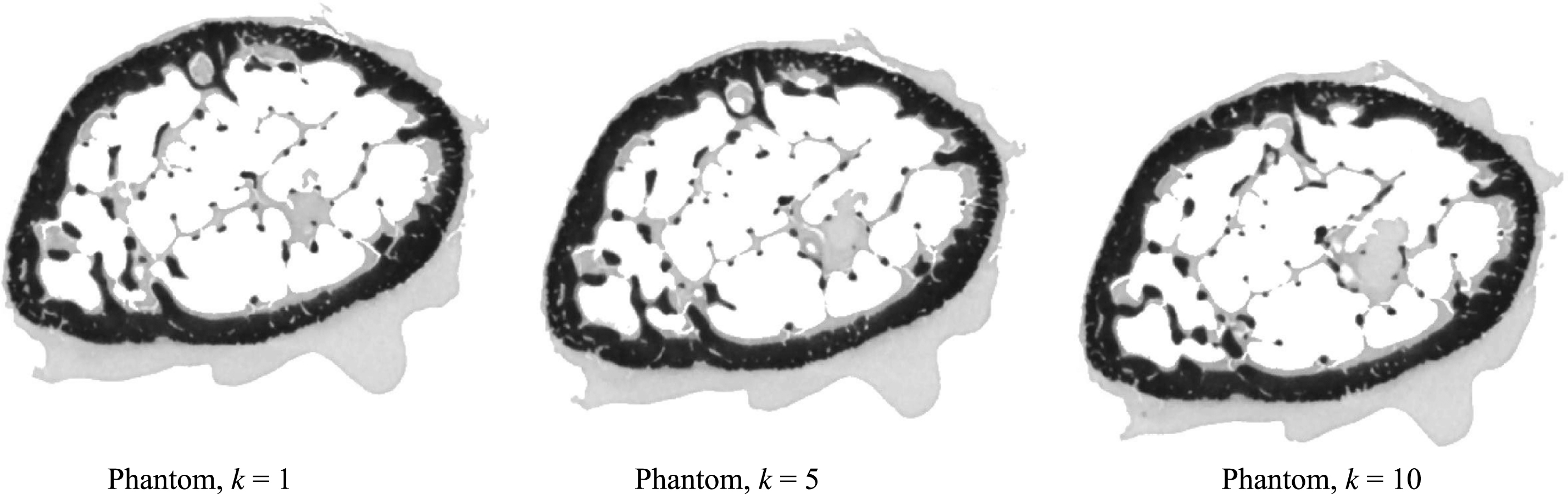
Fig.3
Convergence rate shown for four methods (see Fig. 4). Notably, the CGLS method diverges quickly after 7 iterations while the regularized methods reach semi-convergence point (approximately on the 25th iteration) and then diverge (both RG-B43, 43, 9 and ARG-Bo,9 methods diverge much slower than the RG-B9, 9, 9 method).
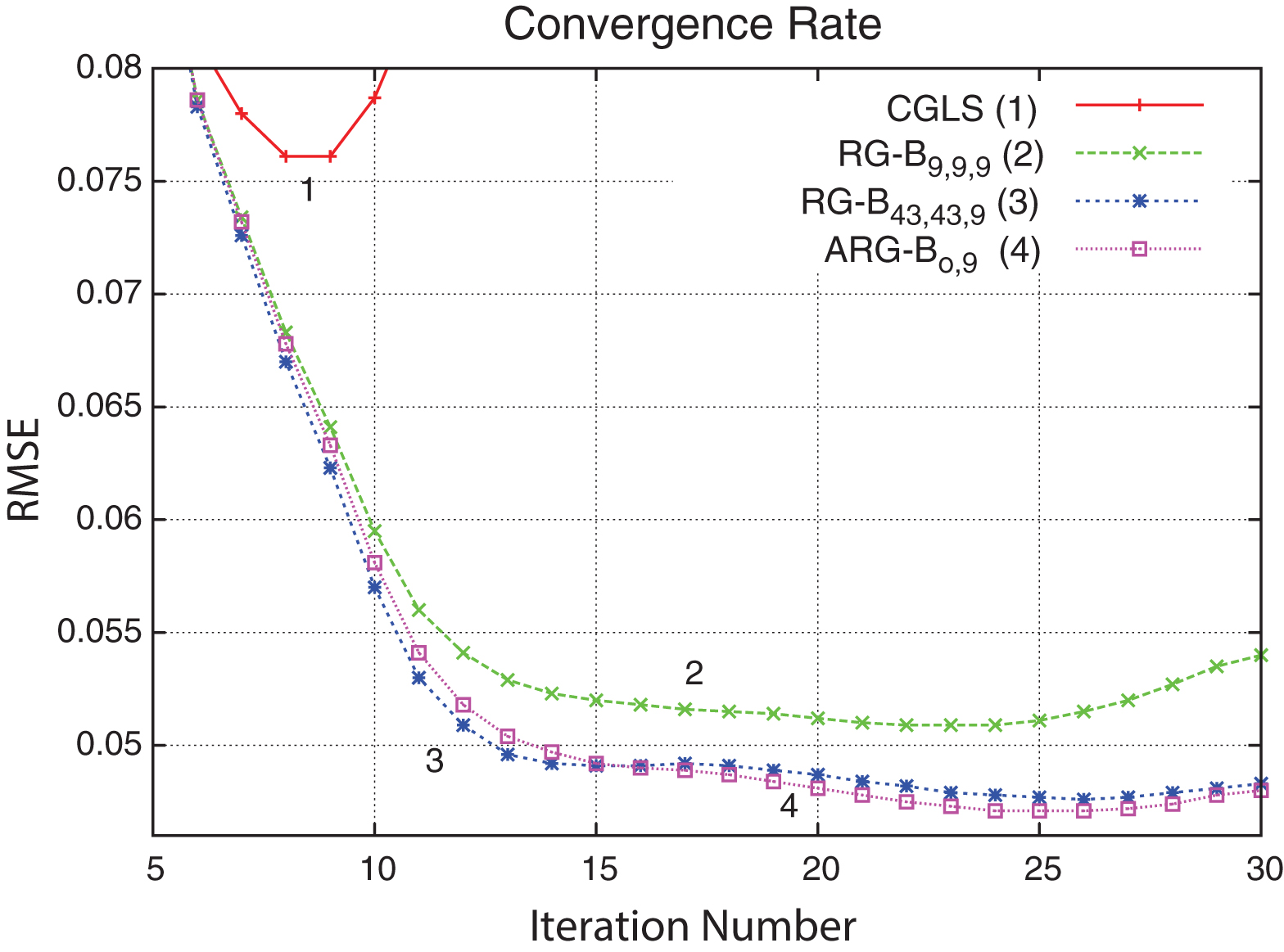
Fig.4
Time frame k = 5 of the phantom in Fig. 2 (middle) is reconstructed using four methods: CGLS, RG-Bsx = 9,sx = 9,sk = 9, RG-B43, 43, 9, ARG-Bo,9. Reconstruction with RG-B9, 9, 9 method is blocky due to absence of the temporal information (small sx = sy = 9 window). Methods RG-B43, 43, 9 and ARG-Bo,9 are similar in the reconstruction quality, however some features are sharper with the ARG-Bo,9 method which is also confirmed by the lower RMSE. The line profiles correspond to the 1D plot in Fig. 5.
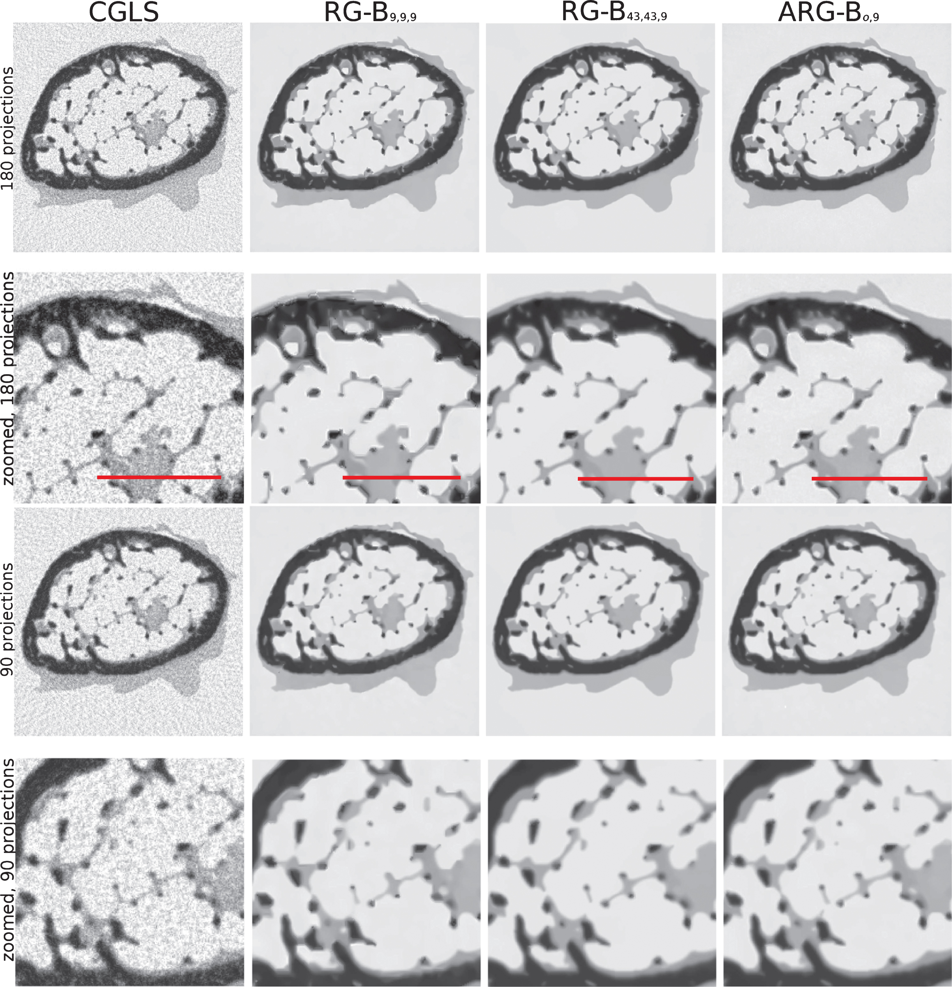
Fig.5
The plot showing the ability to recover image features for four methods (see the line profile in Fig. 4). The proposed method (ARG) shows the best performance to preserve features and denoise the signal.
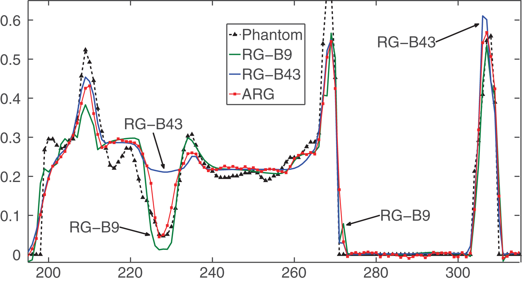
Fig.6
An axial slice taken from one of six volumetric time-frames reconstructed by FBP, CGLS and ARG methods. The ARG reconstruction has improved signal-to-noise ratio and sharp discontinuities between different phases (ice-crystals and air bubbles).
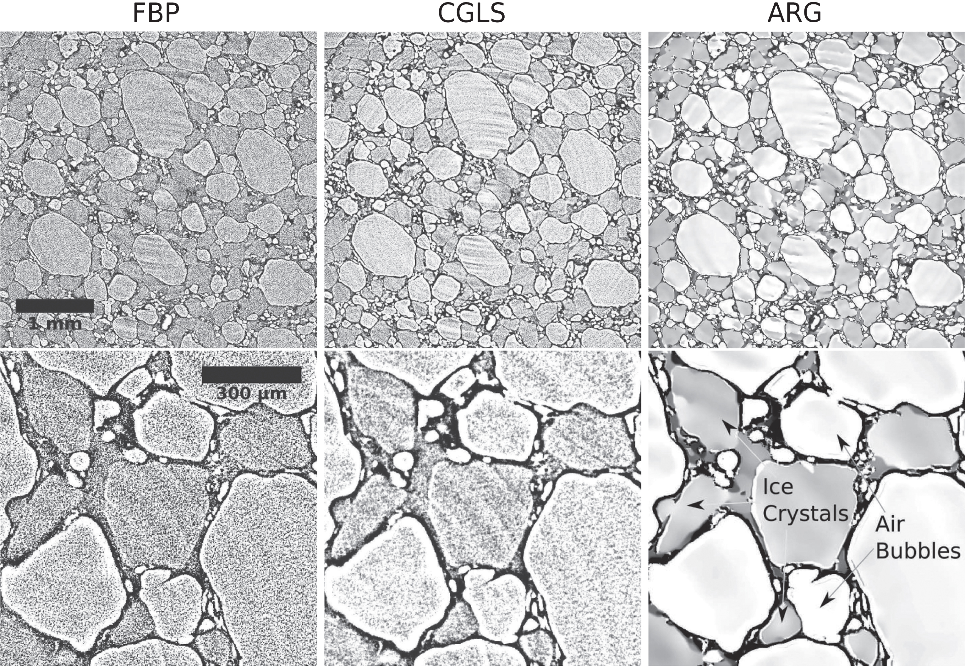
Fig.7
Rendered sub-volumes after segmentation for air bubbles (left) and ice-crystals (right).
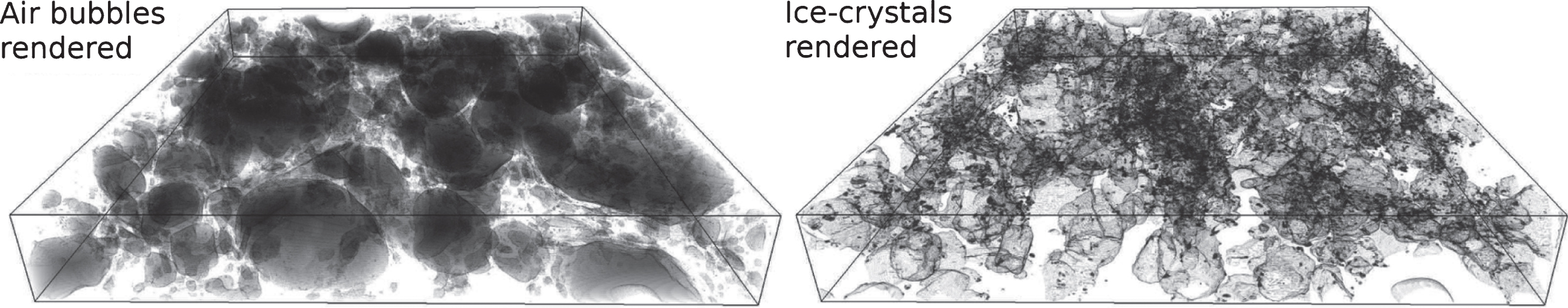
Table 1
Parameters for image reconstruction experiment (Fig. 4)
| Parameters | CGLS | RG-B9, 9, 9 | RG-B43, 43, 9 | ARG-Bo,9 |
| sx | - | 9 | 43 | - |
| sy | - | 9 | 43 | - |
| sk | - | 9 | 9 | 9 |
|
| - | - | - | 9 |
|
| - | - | - | 43 |
| L | - | - | - | 0.4 |
| rx = ry | - | 5 | 5 | 5 |
| β | - | 0.2 | 0.2 | 0.2 |
| h | - | 0.1 | 0.1 | 0.1 |
| CGLS Iterations No. | 8 | 25 | 25 | 25 |
| FP (11) Iterations No. | - | 1 | 1 | 1 |

