
An easily implemented and accurate model for predicting NCAA tournament at-large bids
Abstract
We extend prior research on the at-large bid decisions of the NCAA Men’s Basketball Committee, and estimate an eight-factor probit model that would have correctly identified 178 of 179 at-large teams in-sample over the 2009–2013 seasons, and correctly predicted 68 of 72 bids when used out of-sample for 2014 and 2015. Such performance is found to compare favorably against the projections of upwards of 136 experts and other methodologies over the same time span.
Predictors included in the model are all easily computed, and include the RPI ranking (using the former version of the metric), losses below 0.500 in-conference, wins against the RPI top 25, wins against the RPI second 25, games above 0.500 against the RPI second 25, games above 0.500 against teams ranked 51–100 in RPI, road wins, and being in the Pac-10/12. That Pac-10/12 membership improved model fit and predictive accuracy is consistent with prior literature on bid decisions from 1999–2008.
1Introduction
The NCAA Men’s Basketball Tournament, commonly known simply as the NCAA Tournament, has been a popular topic of academic inquiry. This research has often focused on projecting game winners, overall tournament winners, or progression likelihoods of various seeds; recent examples include Brown and Sokol (2010), Coleman and Lynch (2009), Jacobson et al. (2011), Khatibi et al. (2015), Koenker and Bassett Jr. (2010); Kvam and Sokol (2006); Morris and Bokhari (2012), and West (2006, 2008). This is not surprising, as games and gaming associated with completing a bracket is highly popular even among those who are not normally sports fans or college basketball fans. Each season, more than 60 million people in the U.S. complete a tournament bracket (Geiling, 2014). An estimated $60–70 M is legally wagered on the tournament annually—exceeded only by the Super Bowl (Dizikes, 2014)—and another $3B is bet illegally via pools each year (Rennie, 2014). ESPN’s online tournament projection contest garnered more than 11 million contestants in 2014, a number that included even the president of the United States (Quintong, 2014). The Warren Buffett-backed “Quicken Loans Billion Dollar Bracket Challenge” tournament prediction contest generated as many as 15 million entries in 2014 (Kamisar, 2014) and a 300% increase in brand awareness for Quicken Loans (Horovitz, 2014). The NCAA Tournament thereby captures great attention during the approximately three weeks from the time the playoff bracket is announced until its ultimate winner cuts down the nets after the championship game.
Prior to those three weeks, however, the multi-month process of projecting the teams that will be selected to play in the (currently) 68-team tournament is of prime concern amongst those who are most heavily invested in the sport: players, coaches, athletic directors, conference commissioners, fans, and sports media. Whereas 32 of the 68 teams (in 2015) are invited to play by virtue of winning their respective conference championships, the remaining so-called “at-large” invitees are determined by the NCAA Men’s Basketball Committee, popularly known as the Selection Committee. This 10-person committee is comprised of athletic directors and conference commissioners from amongst the NCAA membership; committee members serve staggered five-year terms (NCAA.org, 2014a). In addition to identifying the at-large teams to be invited, the committee also assigns seeds to each team and places all 68 teams into the playoff bracket.
Although the seeding and bracket placements of the teams can certainly impact the per-game and tournament win probabilities for each participating team, it is the at-large selection process that draws the most attention. Obviously, a team cannot win if it doesn’t participate, and being selected is often viewed in and of itself as the mark of successful season. Participating schools, players, and coaches receive various benefits from being in the tournament; tangible direct benefits currently include a substantial financial reward of approximately $1.58 million, paid out over six years, for each tournament game that a school plays (Smith, 2014). Simply being selected as an at-large invitee guarantees that a minimum of that amount will go into the coffers of the invited school and/or its affiliated conference.
Despite the importance of these selections to major-college basketball’s various stakeholders, and despite the fact that the NCAA has done much in recent years to explain the machinations of the committee as it makes its at-large selections and seeding decisions (NCAA.org, 2012, NCAA.com, 2014), much about the process remains a matter of conjecture. Committee deliberations take place in private closed sessions and little is typically revealed about exactly why a particular team is or is not selected in a given year. In addition, little is disclosed or formalized about which factors are typically viewed as most important to committee members on a year-to-year basis. Given this level of secrecy, combined with the large level of interest in the outcome, projecting which teams the committee will select each year is a popular pursuit. The predictions of 136 experts and/or algorithms were compiled prior to the 2015 tournament at www.BracketMatrix.com (2015), and the projections of widely recognized experts such as Joe Lunardi at ESPN and Jerry Palm of CBS Sports are closely followed by many.
What is comparatively well known about the process is that the NCAA does provide a litany of factors to committee members for their consideration via so-called “team sheets” and “nitty-gritty reports” (NCAA.org, 2012; NCAA.org, 2014b). The focal metric on these reports and the metric used to rank and categorize teams is the Rating Percentage Index (RPI), a weighted average of three factors: (1) the teams’ winning percentage against Division I opponents, (2) the winning percentage of the team’s opponents, and (3) the winning percentage of the team’s opponents’ opponents. These three elements are weighted by 25%, 50%, and 25%, respectively. The latter two components, with relative weights of 66.7% and 33.3%, are also used to calculate a team’s strength of schedule. Prior to 2005, home wins and losses were treated identically to road wins and losses when computing the first element of the RPI. However, since 2005 the NCAA has used an approach by which home wins and road losses count as 0.6 each, and home losses and road wins count as 1.4 each, when computing a team’s winning percentage (Coleman et al., 2010).
2Literature review
In addition to its aforementioned popularity among followers of the sport, the at-large bid selection process has been the subject of academic research. Whereas some of this research has focused on developing improved methods for making the selections (e.g., Fearnhead & Taylor, 2010), there is another line of inquiry over the last 15 years that has focused on attempting to capture the policy of the committee and/or predict its decisions using statistical methods.
Coleman and Lynch (2001) examined 249 potential at-large teams from 1994–1999 and 42 potential predictors, largely representing factors included on the Committee’s nitty-gritty reports. That study generated a six-factor probit model that was 93.7% accurate in-sample and 94% accurate out-of-sample from 2000 through 2005, with performance declining to 89% during 2006–2008 (Coleman, 2015). Coleman, DuMond, and Lynch (2010) later examined 479 at-large candidates from 1999–2008, to investigate conference-based bias in both selections and seeding. A 15-factor probit model estimated from the same 1999–2008 data (Coleman et al., 2011) correctly assigned 96.5% of at-large slots in-sample and 170 of 179 slots (94.9%) out-of-sample from 2009–2013. That same probit model also suggested benefit for teams from the Big 12 and Pac-10/12 and a detriment for teams from the Missouri Valley Conference, favor toward teams with conference commissioners on the committee, and penalty for teams ranked lower in league standings, ceteris paribus. However, out-of-sample model predictions made while omitting these bias terms correctly predicted 73 of 74 slots in 2012-2013, suggesting that the committee biases may have recently waned (Coleman, 2015).
Shapiro et al. (2009) also analyzed the question of bias in the at-large selection process. Using a set of 11 performance statistics as controls, those authors also found bias associated with conference membership during the 1999–2007 period, specifically favoring majors and against mid-majors. In another consistency with the Coleman et al. 1999–2008 analyses, they found a relationship between bids and where teams finished in their league standings. They found no relationship between selections and the geographic region, per capita income, or population of candidate teams, nor with the school’s number of tournament appearances in the preceding 10 years. Their logistic regression model miss-assigned 15 at-large slots in-sample from 1999–2007, although the authors report no out-of-sample results.
In a more recent assessment, Paul and Wilson (2012) focused on whether the bias findings in Coleman et al. (2010) resulted from the use of the RPI as the control for team performance, as opposed to a performance metric that takes into account margin of victory. Paul and Wilson find that a factor representing any sort of representation on the committee, as well as two indicators representing affiliations with mid-major and small conferences, respectively, were not significant in the presence of the Sagarin Predictor ranking as the sole control, whereas they were significant in the presence of the RPI as the sole control. The authors’ use of a different time frame (2004–2011) for their study vis-à-vis the Coleman et al. (2010, 2011) window of 1999–2008 raises the question of whether the bias found in the latter study was largely the result of committee behavior before 2004.1 The authors do not report in-sample or out-of-sample predictive results for their models, although the McFadden r-square of their best model (which included the Sagarin Predictor) was 0.7307.
The only other known published analysis of at-large bids is the work of Leman et al. (2014), who analyzed the 2010 and 2011 selections. Leman et al. found that the Predictor, Elo, and overall rankings of Sagarin, as well as the Logistic Regression/Markov Chain (LRMC) method of Kvam and Sokol (2006) and Sokol and Brown (2010), not to be significant in the presence of the current (post-2004) version of the RPI. They also found that treating the winning percentage and strength of schedule components of the current RPI separately— noting that both values reflect the current RPI’s approach of weighting wins and losses differently at home versus those on the road— and allowing the weighting scheme to differ from the 25 : 75 ratio prescribed in the RPI, generates stronger expected predictions that when using the RPI as prescribed by the NCAA. Specifically, the committee’s implied relative weight on strength of schedule is estimated to be approximately four times as large as the implied weight on the winning percentage. The authors also investigated the presence of a marquee factor in tournament selections over the 1994–2010 period, and find that marquee teams obtain bids more readily over and above what would be expected according to the current RPI’s winning percentage and strength of schedule components.2
The current research seeks to improve on the earlier bid prediction research described above by examining 15 years of committee bids from 1999–2013, which includes recent seasons and data not previously examined in the literature.
3Data and variables
Table 1 describes all potential predictors included in the analysis, which are similar to those employed in the Coleman et al. (2010, 2011) evaluations of 1999–2008 at-large bids. Scores and game sites were collected from KenPom.com. RPI values and corresponding metrics for each team were computed using the RPI formula that was in use prior to 2005, which weights wins and losses equally whether home or away. Corresponding metrics according to the current version of the RPI were collected from CollegeRPI.com and CBSSports.com. Sagarin rankings were collected from USA Today.
The outcome measures employed throughout the analysis was a binary variable (BID) reflecting whether a team received an at-large bid to the tournament.
4Analysis
The objective of the analysis was a model that would predict future at-large bids as accurately as possible. Typically this would imply the selection of a model based on the best value of an information criterion such as Akaike’s Information Criterion (AIC), or a model with the best cross-validation performance,3 with the p-values of the predictors being comparatively unimportant vis-à-vis typical hypothesis testing thresholds (Shtatland et al., 2001). However, because a predictive model in the current context has potential use as a decision aid by the selection committee as well as by administrative personnel such as athletic directors and coaches, and strong prospective attention from the media and the college basketball public, the acceptability of the model to such an array of constituencies was a concern. Thus, consistent with the approaches in Coleman et al. (2001, 2011), the face validity of the model, as proxied by the p-values and the expected signs of its predictors, was a consideration in addition to its predictive accuracy.4 For ease of reference, in the following discussion we occasionally use these p-values along with traditional hypothesis testing thresholds to refer to the “significance” of various predictors. However, it should be noted that the multicollinearity among many of the predictors inflates standard errors and disturbs inferences, and thus tests for statistical significance may not be valid. Moreover, the best model for prediction that we seek here is not necessarily the best model for discussing the statistical significance of its factors.
Predictive accuracy was determined by the number of at-large bids missed using leave-one-year-out cross-validation. In this process, strong candidate models according to the AIC and the number of at-large bids missed in-sample were iteratively estimated while leaving out one year of data at a time. Each of these estimations was then used to predict at-large bids in the respective omitted year. The cumulative number of at-large bids missed over the omitted years represented the cross-validation performance as well as the expected predictive accuracy out of sample.
A sample of 243 potential at-large bid candidates from 2009–2013 was initially examined, as these years represent selections beyond those previously analyzed in the Coleman et al. (2010, 2011) modeling. Also as in earlier Coleman et al. (2001, 2010, 2011) modeling, the analysis focused only on those bid-eligible teams in each season with RPI values ranked between 20 and 80, to distinguish selections involving teams that had at least some reasonable possibility of being selected. To account for the increase in the number of at-large bids from 34 to 37 starting in 2011, a control variable BIDS37 (1 for years 2011–2013, 0 otherwise) was added to all model specifications.
Given that the pre-2005 version of the RPI was used in the prior Coleman et al. studies of at-large bid decisions, we first examined whether recent committee decisions have been more aligned with the newer version. A probit model was fit using only the former RPI ranking with BIDS37, and then again using only the current RPI ranking with BIDS37. The former RPI ranking had better fit metrics (AIC of 116.4 vs. 152.6), a larger coefficient (–0.1326 vs. –0.0929), and missed fewer at-large slots in-sample (12 vs. 15) and during leave-one-year out cross-validation (12 vs. 15) than did the new version. Thus, the former version of the RPI was used throughout the bid modeling described below.
To winnow the predictor list, a stepwise probit was first performed using the team performance factors in Table 1 and α= 0.10 to enter and exit. The result of the stepwise procedure was used as a basis for further analysis, and is shown as equation (1) in Table 2. Predictors selected by the stepwise included the RPI ranking (RPIRANK), losses below 0.500 in-conference (CONFBELOW500),5 wins against the RPI top 25 (T25WINS), wins against the RPI second 25 (T50WINS), games above 0.500 against teams ranked 51–100 in RPI (T100ABOVE500),6 and number of road wins (ROADWIN). Ranking at-large candidates according to equation (1) missed five out of 179 at-large slots in-sample, or an average of one per year from 2009 through 2013. Leave-one-year-out cross-validation yielded six at-large bids missed over the same time period.
In order to check whether equation (1) is the result of an over-fit to 2009–2013, the model was then fit to the full 1999–2013 data set (n = 721), omitting New Mexico in 1999 as an outlier: it had the lowest RPI ranking (74th) of any team selected in the 15-year period, its athletic director was on the committee (Coleman et al., 2010), and it received a 9-seed, implying that it was not even one of the last few teams to make the field. All team performance factors were significant (four with p < 0.0001, and two with p < 0.001), indicating that the significance of these factors is not isolated to the period 2009–2013.
However, using the 15-year estimation for predictive purposes raises concerns given the evidence of conference biases found previously for 1999–2008. That the 15-year fit misses only five slots in 2009–2013 (same as the five-year fit), and misses 25 during 1999–2008, clearly suggests that the selection process has been fundamentally different recently, a finding that is consistent with those of Paul and Wilson (2012) for 2004–2011.
In order to address further the questions of whether adjustments for bias still need to be included in the current selection estimations, as well as the time window on which the model should be estimated, we investigated all 30 at-large misses of the 15-year fit during 1999–2013 vis-á-vis each conference. The four most extreme cases of possible imbalance in the treatment of a conference were the Pac-10/12 (six times it received favorable treatment— meaning one of its teams got a bid that the model predicted should not— and in no case did it receive detrimental treatment in which a team failed to receive a bid that the model predicted), the Big East (none favorable, four detrimental), the ACC (four favorable, none detrimental) and the Missouri Valley (one favorable, seven detrimental). However, a closer examination of the misses indicated that the Pac-10/12 was the only league with misses that were rather consistent across time, included recent years, and involved a variety of schools. A Pac-10/12 team received a bid that was not expected by the 15-year model in 2004 (Washington), 2006 (California), 2007 (Stanford), 2008 (Oregon), 2009 (Arizona), and 2011 (Southern California).7 Conversely, the Big East’s misses on the down side involved four different teams, but none since 2007. The ACC misses involved three teams in only three different years, and the Missouri Valley (MVC) misses involved four teams, but none since 2008.
To further investigate bias involving these four leagues, their respective binary variables were added to the 15-year model. Given that the 1999–2008 findings from Coleman et al. (2011) also indicated that having representation on the committee was significant to bids, each of the three committee representation factors was also added. The Pac-10/12, Big East, and MVC were significant, along with having the conference commissioner on the committee (CONFONCOMM)— the latter confirming the findings of Coleman et al. (2011). However, to determine a best predictive model for future years, the salient question is whether this pattern remains sufficiently persistent in recent time windows to conclude that it will continue. To address this issue, we iteratively estimated the 15-year model with P10, BE, MVC, and CONFONCOMM collectively added, to incrementally shorter and more recent time frames, from 1999–2013 to the 2009–2013 period. In the process, the results of which are summarized in Fig. 1, having the conference commissioner on the committee became insignificant when fit to the 2002–2013 time period, the Big East indicator went insignificant when fit to 2004–2013, and the MVC indicator went insignificant when fit to 2008–2013. The Pac-10/12 factor was the only bias-related factor that remained significant in every time window analyzed. In addition, all team performance factors in (3) maintained their significance at least at the 0.10 level throughout. We thus re-ran the equation (1) estimation for 2009–2013 while adding the Pac-10/12 factor (P10). The result is shown as equation (2) in Table 2.
Equation (2) missed just two slots in-sample, both in 2011, meaning that the model was perfect for four of the five in-sample years. During leave-one-year-out cross-validation, equation (2) missed five at-large slots, a one-bid improvement over equation (1). Moreover, when fit to the 15-year data, all seven factors retained significance (the first four team performance factors with p < 0.0001, the last two with p < 0.001). Although the number of conference losses below 0.500 in the league (CONFBELOW500) was not as strong (p = 0.1062), this factor was retained in the model, given its significance in all bid model estimations extending back further than five years (p < 0.0001 for any time frame beyond six years.)
To equation (2) we added each of the remaining predictors individually, and estimated fits over the 2009–2013 period. The only team performance factor with p < 0.05 in the presence of the factors in (2) was the number of wins above 0.500 against teams ranked 26–50 in RPI (T50ABOVE500), which was thus added to the model. The revised 2009–2013 estimation is shown as equation (3) in Table 2. Although the number of conference losses below 0.500 in the league (CONFBELOW500) remained just outside significance (p = 0.1012), this factor was again retained in the model, given its significance over longer time frames. All factors were significant over the 15-year estimation as well.
Equation (3) misses only one at-large slot in the entire five-year interval: the model errs on Florida State’s selection in 2011. The Atlantic Coast Conference (ACC) and MIDMAJOR binary indicators are the only remaining predictors with p < 0.05 over 2009–2013 when added to (3), but neither was significant when the model is estimated over the full 15 years of data. (The ACC’s significance during 2009–2013 is likely heavily influenced by the Florida State miss in 2011.) Thus, neither of these factors was added to the model.
Leave-one-year-out cross-validation indicated that equation (3) misses four spots: one in 2010 (first team out), two in 2011 (first and fifth team out), and one in 2012 (first team out). These results suggest an expected out-of-sample accuracy of less than one slot missed per year.8
5Alternate model selection processes
Given that the above model selection process was not based strictly on the minimization of a criterion (e.g., the AIC) associated with predictive accuracy, two additional model selection processes were employed to generate alternate specifications for comparison. The first of these used a stepwise approach with α= 0.157 to enter and exit, given that such a method asymptotically approaches the use of the AIC as a model selection criterion as the sample size increases (Shtatland et al., 2001). All factors in Table 1, including the conference and committee affiliation factors, were included in the stepwise as potential predictors. The result was a model with identical predictors to those in equation (3), but with CONFBELOW500 deleted and POWER6 added. The AIC of this alternate model was 48.655, which was slightly worse than equation (3)’s AIC of 47.702. The model missed two at-large slots in-sample, which was one worse than equation (3), and a leave-one-year-out cross-validation generated five misses, also one worse than equation (3). Thus, this alternate specification was deemed not to be superior toequation (3).
A second alternate selection was done using a stepwise process described in Shtatland et al. (2001), in which α= 1.00 is used to enter and exit. The result is a sequential series of models from which to choose. The first 20 steps of the stepwise sequence are summarized in Table 3, along with the associated AIC values and results of a leave-one-year-out cross-validation of each of the 20 models identified.9 The sequence identified 13 alternate models with AIC values better than equation (3)’s value of 47.709; however, none of these had better cross-validation results than equation (3)’s four misses. The best model from the sequence yielded complete separation of the data (i.e., no at-large misses) in-sample,10 and an AIC of 30.329 from the last iteration of the model fitting process. Both values are obviously better than those from equation (3). This best model contained all the predictors in equation (3), but also added the conference affiliation factors ACC, BE, and B10. However, the leave-one-year-out cross-validation of this alternate model yielded six at-large misses, versus the four of equation (3)—even though all five fits in the cross-validation yielded complete separation of the in-sample data. Because of the inferior cross-validation performance of this and all other models shown in Table 3, none of these alternate specifications were determined to be better predictors of at-large tournament bids than equation (3).11
6Considering alternate rankings
Pursuant to the findings of Paul and Wilson (2012) regarding the committee’s apparently greater reliance on rankings that consider margin of victory than on the RPI, equation (3) was iteratively re-fit while using the ranking of each of 25 different mathematical systems in place of RPIRANK. The list of ranking methods employed is shown in Table 4.12 The 25 systems employed were all those with pre-tournament rankings compiled at Massey (2013) for every year from 2009 through 2013. Some of these— e.g., the aforementioned LRMC model, the Sagarin ranking, and the ranking of Ken Pomeroy— have been shown to be superior predictors of tournament performance (Kvam & Sokol, 2006; Brown & Sokol, 2010), are well-known and respected in basketball circles, and are reportedly provided to the committee during its deliberations (NCAA, 2014b). However, the best AIC value for any of these fits was 79.3 (when using the BPI ranking13), compared to the 47.7 value of equation (3). Moreover, estimations of models using each individual ranking as the sole predictor of bids (in addition to the control variable BIDS37) indicated that none of the alternative ranking systems yielded an AIC superior to that of RPIRANK when it was used as the lone predictor (116.4).
Each of the 25 systems was also added individually to equation (3) as an additional predictor (i.e., not in place of RPIRANK). While the collinearity between RPIRANK and any of these systems is obviously high, only eight had p-values less than 0.05 in the expected direction in the presence of the equation (3) factors: BOB, CNG, DCI, DOK, LMC, POM, RTH, and STH. In all eight cases RPIRANK was also significant, with a coefficient that ranged from 3.11 to 5.61 times as large as the coefficient of the alternate ranking. As a further confirmation of the choice of the previous version of the RPI in the development of equation (3), when the current version of the RPI was also added to equation (3) as an additional predictor, its p-value approached 1.00, the coefficient of RPIRANK was over 1000 times as large (and with an unexpected sign), and the p-values of the predictors in equation (3) remained significant.14 These findings collectively suggest that committee decisions during 2009–2013 align more so with the RPI— and specifically the former version of the RPI— than with metrics that account for margin of victory or with the current RPI.
However, in order to check whether adding an alternate ranking to equation (3) would improve its predictive capacity, further investigation was made of the alternate rankings that yielded the best fits when added to equation (3). When STH is added to equation (3), the AIC improves from 47.7 to 35.2, with no bids missed in-sample— better than equation (3) on both metrics. However, leave-one-year-out cross-validation yielded four misses, the same as equation (3). Equation (3)’s AIC drops from 47.7 to 35.7, with one bid missed in-sample, when DCI is added to the model. The leave-out-year-out cross-validation yielded three misses, better than equation (3), with complete separation of the data achieved when omitting any year other than 2013. However, due to the small incremental gain in cross-validation accuracy vis-à-vis equation (3), as well as the comparative difficulty of implementing a model for real-time predictive purposes that includes an alternate ranking that (unlike RPIRANK) is not easily replicated independently or rapidly, including DCI was not deemed a preferable option.15
7Comparison to other methods
In order to provide some context for the equation (3) in-sample accuracies reported above, the model’s number of at-large misses was compared to the number of misses generated by the experts and various methodologies compiled at www.BracketMatrix.com over the same time period. For each individual year, equation (3)’s accuracy would have tied for best versus all methodologies compiled for that year. Of the 21 systems with reported results for all years during 2009–2013, the lowest number of misses was six. Thus, equation (3)’s one in-sample miss, as well as its four misses in the leave-one-year-out cross-validation, would have been superior to all other methods and experts. Similar results are found if the comparison is made over the incrementally more recent 2010-13, 2011-13, and 2012-13 time windows, where the best performance reported by any other method was five misses (among 36 systems), three misses (among 51 systems), and one miss (among 81 systems), respectively. Over any of these windows, the misses from equation (3), whether in-sample or in the cross-validation, would have been as good or better than the best of the other approaches.
8Out-of-sample performance
A similar comparison was made using the 2014 and 2015 selections as an out-of-sample assessment. Equation (3) correctly predicted 35 of the 36 at-large bids for 2014, missing only on North Carolina State (it predicted California to receive that bid instead). Only one of the 120 methods compiled by BracketMatrix.com in 2014 did better. Nearly all (117 of 120) of those other methods missed on North Carolina State as well, suggesting that the choice of North Carolina State was likely a matter of the committee simply deviating from its historical norms, and not a result of error in the modeling of those norms.
In 2015, equation (3) correctly predicted 33 of 36 bids, missing on Boise State, Dayton, and UCLA (it predicted Temple, Colorado State, and Miami (FL) to get those bids instead). All but 14 of 136 methods at BracketMatrix.com missed on UCLA as well, and 122 of the 136 projected Temple to be chosen even though the Owls were not. These findings suggest that the UCLA and Temple miss-assignments were again likely a result of the committee significantly deviating from its historical patterns, and not a result of modeling error. That Boise State and Dayton were equation (3)’s first two teams out of the field, whereas they were the last two teams in the field in reality (Patterson, 2015), also suggests that despite missing on these teams the model had their bid prospects estimated closely.
Equation (3)’s 33-of-36 performance in 2015 was surpassed by 124 of 136 methods at BracketMatrix.com, suggesting that the model was relatively poor in 2015. However, a closer examination indicated that this deviation vis-à-vis the performance of other methods was largely the result of Equation (3)’s treatment of Dayton: had the model been correct on Dayton, only 13 of the 136 other methods would have beaten it. All 136 other methods at BracketMatrix.com projected Dayton to be chosen, with an average expected seed of 8.79; 110 of 136 methods had Dayton seeded no worse than 9. Such a placement suggests that these methods had Dayton at least 10 ranking positions above the cut line for at-large bids in 2015, which was between the 46th- and 47th-ranked teams (Patterson, 2015). In contrast, equation (3) predicted Dayton to be the second team left out (i.e., essentially the equivalent of 48th). As noted above, Dayton was ultimately the last team to make the field. Thus, equation (3) had Dayton within two ranking positions of their placement by the committee, which was actually a much more accurate reflection of their relative ranking by the committee than 110 of 136 other methods. This finding indicates that despite missing on Dayton, equation (3) assessed the at-large prospects of Dayton more appropriately than most other methods.
In sum, of equation (3)’s four out-of-sample prediction errors over 2014 and 2015, two appear to be substantial deviations of the committee from its historical patterns, a third (Boise State) was the model’s first team out, and the fourth (Dayton) was the model’s second team out, and one that the model placed more accurately than the large majority of experts and methods.
9Discussion and conclusion
Equation (3) appears to be a strong model of the at-large bid selection process. Its strength is a signal that the committee’s decisions are very consistent year-to-year despite the partial changeover in committee membership each year. In addition to its strong fit, its simplicity and easy replicability make it even more attractive as a predictive tool and as a potential decision aid to the selection committee. Given the wide-spread understanding of the way that the RPI is computed among those heavily involved in the sport, the predictors in the model have the added benefits of transparency and understandability, perhaps most significantly among the selection committee members themselves. This would not necessarily be true had other rankings been employed as predictors.
Equation (3)’s attractiveness for potential use is also enhanced by its strong face-validity. For example, and as one would expect, the weight placed on wins against top 25 opponents (2.7509) is higher than the weight placed on wins against teams ranked 26–50 (1.2572). Similarly, the weight assigned to wins above 0.500 against teams ranked 26–50 is higher than the implied weight for wins above 0.500 against teams ranked 51–100 (1.2021 vs. 0.8364, respectively). It is also likely satisfying to those invested in the sport to find that wins against top 25 teams and wins on the road are apparently rewarded, whereby losses in such settings are not penalized. The same could be said of wins against teams ranked 26–50 getting consideration even if a team has a losing record against that same group. It is also likely unsurprising and welcomed that losses are also considered when examining performance against teams ranked 26–50 or 51–100, but a winning record is rewarded while a losing record is not penalized. Although the committee’s apparent penalizing of teams with losing conference records is evidence of behavior that is inconsistent with proclamations that the committee does not consider league membership or league standings (ASAPsports.com, 2015), this violation of stated procedures is one that many in the sport would likely findpalatable.
Notes
1 Differences between the Paul and Wilson (2012) and Coleman et al. (2010) findings regarding committee bias could also be the result of other differences in the modeling approaches between the two papers. For example, Paul and Wilson used the current version of the RPI (the one in use since 2005), in which road wins and losses are weighted differently from home wins and losses, versus Coleman et al.’s use of the previous version of the RPI that weights wins and losses the same regardless of site. Paul and Wilson also did not control for as many additional factors that have been suggested by other previous literature or by the current research to be related to committee bids.
2 Leman et al. focus on the case of Virginia Tech in 2010, and find that had Virginia Tech been a marquee team, their probability of a bid would have increased from 28% to 86%.
3 The AIC has been shown to be asymptotically equal to leave-one-out cross-validation (Shtatland et al., 2001).
4 As will be discussed later, the expected predictive accuracy of the model generated by this methodology was ultimately compared to the expected predictive accuracy of alternate model selections driven strictly by the minimization of the AIC.
5 As an example, a conference record of 8–10 would result in a CONFBELOW500 value of |8–10| = 2.
6 As an example, a record of 4-1 against teams ranked 51–100 in RPI would result in a T100ABOVE500 value of 4–1 = 3.
7 Any evidence of apparent bias in favor of the Pac-10/12 could be instead a result of, or a proxy for, other effects not captured in the model. However, the involvement of six different Pac-10/12 schools – none of which were UCLA, and only two of which (Arizona and arguably Stanford) might have been considered a perennial power at the time of selection – suggests that any such bias is not likely a result of the type of team-specific marquee factor discussed by Leman et al. (2014).
8 POWER6 was not significant when added to equation (3), and particularly so when added to an estimation fit to the full 15 years of data. However, its addition did improve the AIC to 26.971 over 2009–2013, and achieved complete separation of the in-sample data. The AIC and in-sample bids missed were both better than equation (3). Leave-one-year-out cross-validation yielded four misses, the same as equation (3), although complete separation of the data was achieved on all five fits. Due to the issue of complete data separation, a cross-validation using Firth’s bias adjustment was performed, and it also yielded four misses, the same as equation (3). Because of the lack of improvement in cross-validation performance versus equation (3), POWER6 was not added to the model.
9 All models in further steps of the sequence had AIC values worse than equation (3).
10 Each of the last 10 models reported in Table 3 also yielded complete separation of the in-sample data.
11 The lowest-AIC model from the sequential stepwise process was also fit using Firth’s bias adjustment. The Firth-adjusted version missed one at-large spot in-sample— the same as equation (3). When the leave-one-year-out cross-validation was also replicated using the Firth adjustment on all estimations, the model missed six at-large spots, two worse than equation (3). Thus, equation (3) was again determined to be a more favorable model choice. That equation (3) generated better cross-validation performance while also including fewer predictors also made it more favorable per an Occam’s razor principle.
12 The list of 25 alternate rankings includes the Sagarin ranking, which was already considered during the model development described in previous sub-sections.
13 Note that the ranking denoted as BPI here and in Table 4 is not the College Basketball Power Index ranking developed and published by ESPN, which first appeared in 2013.
14 The p-value of CONFBELOW500 remained just above 0.10, and nearly identical to its value in equation (3).
15 When DCI is added to equation (3), two factors exhibit very high p-values: CONFBELOW500 and P10. While this is not necessarily a concern predictively, it does affect the face-validity and thereby the preferability of this specification. Dropping these two predictors from the model yields a worse AIC (39.045), two misses in-sample, and four misses in cross-validation.
References
1 | ASAPsports.com, 2015. National Collegiate Athletic Association media conference March 15, 2015: Scott Barnes. Retrieved April 6, 2015, http://www.asapsports.com/show_conference.php?id=107367. |
2 | BracketMatrix.com, 2015. The bracket project. Retrieved April 6, 2015, from http://bracketproject.blogspot.com/2013/11/the-2014-bracket-matrix-links.html. |
3 | Brown M. , & Sokol J. , (2010) . An improved LRMC method for NCAA basketball prediction. Journal of Quantitative Analysis in Sports. 6: (3), 1–23. |
4 | Coleman B. J. , (2015) . NCAA men’s basketball tournament dance card. Retrieved April 6, 2015, from http://www.unf.edu/~jcoleman/dance.htm. |
5 | Coleman B. J. , DuMond J. M. , & Lynch A. K. , (2010) . Evidence of bias in NCAA tournament selection and seeding. Managerial and Decision Economics. 31: (7), 431–452. |
6 | Coleman B. J. , DuMond J. M. , & Lynch A. K. , (2011) . Invited presentation: Foul on the committee? Investigating and predicting NCAA tournament selection committee decisions, Joint Statistical Meetings (American Statistical Association), Miami, August 3. |
7 | Coleman B. J. , & Lynch A. K. , (2001) . Identifying the NCAA tournament ‘dance card’. Interfaces. 31: (3), 76–86. |
8 | Coleman B. J. , & Lynch A. K. , (2009) . NCAA tournament games: The real nitty-gritty. Journal of Quantitative Analysis in Sports. 5: (3). doi: 10.2202/1559-0410.1165 |
9 | Carlin B. P. , (1996) . Improved NCAA basketball tournament modeling via point spread and team strength. The American Statistician. 50: (1), 39–43. |
10 | Dizikes P. , (2014) . Into the pool: NCAA tourney betting booms. Retrieved April 6, 2015 from http://abcnews.go.com/Business/story?id=88479 |
11 | Fearnhead P. , & Taylor B. M. , (2010) . Calculating strength of schedule, and choosing teams for march madness. The American Statistician. 64: (2), 108–115. |
12 | Geiling N. , (2014) . When did filling out a march madness bracket become popular? Retrieved April 6, 2015 from http://www.smithsonianmag.com/history/when-did-filling-out-march-madness-bracket-become-popular-180950162/?no-ist |
13 | Horovitz B. , (2014) . Quicken Loans’ billion-dollar gamble pays off. Retrieved April 6, 2015 from http://www.usatoday.com/story/money/business/2014/03/25/quicken-loans-march-madness-warren-buffett/6874083/ |
14 | Jacobson S. H. , Nikolaev A. G. , King D. M. , & Lee A. J. , (2011) . Seed distributions for the NCAA men’s basketball tournament. Omega. 39: (6), 719–724. |
15 | Kamisar B. , (2014) . No perfect march madness brackets left in Warren Buffett’s billion-dollar contest. Retrieved April 6, 2015 from http://thescoopblog.dallasnews.com/2014/03/just-16-brackets-still-in-running-for-warren-buffetts-billion.html/ |
16 | Khatibi A. , King D. M. , & Jacobson S. H. , (2015) . Modeling the winning seed distribution of the NCAA division I men’s basketball tournament. Omega. 50: , 141–148. |
17 | Koenker R. , & Bassett G. W. Jr. , (2010) . March madness, quantile regression bracketology, and the Hayek hypothesis. Journal of Business and Economic Statistics. 28: (1), 26–35. |
18 | Kvam P. , & Sokol J. , (2006) . A logistic regression/markov chain Model for NCAA basketball. Naval Research Logistics. 53: , 788–803. |
19 | Leman S. C. , House L. , Szarka J. , & Nelson H. , (2014) . Life on the bubble: Who’s in and who’s out of march madness? Journal of Quantitative Analysis in Sports. 10: (3), 315–328. |
20 | Massey K. , (2013) . Retrieved March 18, 2013, from http://masseyratings.com/cb/arch/ |
21 | Morris T. L. , & Bokhari F. H. , (2012) . The dreaded middle seeds – are they the worst seeds in the NCAA basketball tournament? Journal of Quantitative Analysis in Sports. 8: (2). doi: 10.1515/1559-0410.1343 |
22 | NCAA.com, 2014. Media learns new bracketing principles during NCAA tourney mock selection. Retrieved October 9, 2014, from http://www.ncaa.com/news/basketball-men/article/2014-02-14/media-learns-new-bracketing-principles-during-ncaa-tourney |
23 | NCAA.org, 2012. Basketball committees offer more access to selection materials. Retrieved October 9, 2014, from http://www.ncaa.org/about/resources/media-center/news/basketball-committees-offer-more-access-selection-materials |
24 | NCAA.org, 2014a. Men’s basketball selections 101 – committee. Retrieved October 9, 2014 from http://www.ncaa.org/about/resources/media-center/mens-basketball-selections-101-committee |
25 | NCAA.org, 2014b. Men’s basketball selections 101 – selections. Retrieved October 9, 2014, from http://www.ncaa.org/about/resources/media-center/mens-basketball-selections-101-selections. |
26 | Patterson C. , (2015) . NCAA tournament: Selection committee releases 1-68 ranking. Retrieved April 6, 2015 from http://www.cbssports.com/collegebasketball/eye-on-college-basketball/25109120/ncaa-tournament-selection-committee-releases-1-68-ranking |
27 | Paul R. J. , & Wilson M. , (2012) . Political correctness, selection bias, and the NCAA basketball tournament. Journal of Sports Economics. 16: (2), 201–213. |
28 | Quintong J. , (2014) . Tournament challenge: UConn’s title. Retrieved April 6, 2015, from http://espn.go.com/blog/collegebasketballnation/post/_/id/98364/tournament-challenge-uconns-title |
29 | Rennie M. , (2014) . Nine things you need to know before filling out your NCAA tournament bracket. Retrieved April 6, 2015, from http://www.washingtonpost.com/blogs/early-lead/wp/2014/03/19/nine-things-you-need-to-know-before-filling-out-your-ncaa-tournament-bracket/ |
30 | Sanders S. , (2007) . A cheap ticket to the dance: Systematic bias in college basketball’s ratings percentage index. Economics Bulletin. 4: , 1–7. |
31 | Shapiro S. L. , Drayer J. , Dwyer B. , & Morse A. L. , (2009) . Punching a ticket to the big dance: A critical analysis of at-large selection into the NCAA division I men’s basketball tournament. Journal of Issues in Intercollegiate Athletics. 2: , 46–63. |
32 | Shtatland E. S. , Cain E. , & Barton M. B. , (2001) . The perils of stepwise regression and howto escape them using information criteria and the output delivery system. SAS Users Group International Proceedings. RetrievedNovember 5, 2015, from http://www2.sas.com/proceedings/sugi26/p222-26.pdf |
33 | Smith C. , (2014) . How a single NCAA tournament win is worth $1.6 Million. Retrieved April 6, 2015 from http://www.forbes.com/sites/chrissmith/2014/03/20/how-a-single-ncaa-tournament-win-is-worth-1-6-million/ |
34 | West B. T. , (2006) . A simple and flexible rating method for predicting success in the NCAA basketball tournament. Journal of Quantitative Analysis in Sports. 2: (3), Article 3. |
35 | West B. T. , (2008) . A simple and flexible rating method for predicting success in the NCAA basketball tournament: Updated results from 2007. Journal of Quantitative Analysis in Sports. 4: (2), Article 8. |
Figures and Tables
Fig.1
p-values of conference and committee representation factors found to be significant during 1999–2013 when added to equation (1), when fit to progressively shorter time frames.
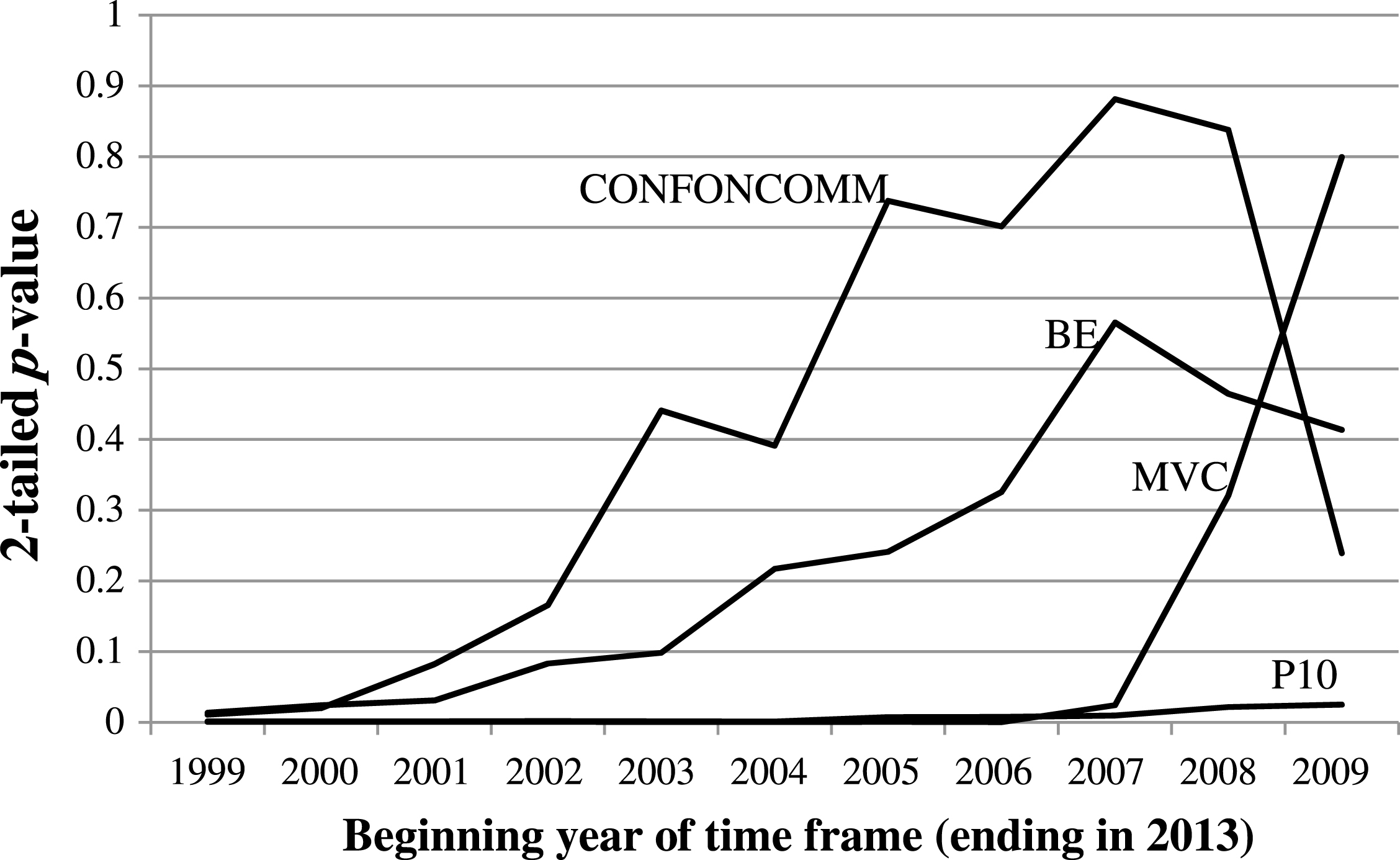
Table 1
Factors hypothesized to be related to at-large bids
| Variable | Abbreviation |
| Rank according to Jeff Sagarin | SAGARIN |
| Overall RPI value (using RPI formula in use prior to 2005) | RPI |
| Overall RPI rank (using RPI formula in use prior to 2005) | RPIRANK |
| Win percentage against Division 1 opponents (first element of RPI) | WINPERC |
| Strength of schedule (final two elements of RPI) | SOS |
| Strength of schedule rank | SOSRANK |
| No. of conference wins | CONFWIN |
| No. of conference losses | CONFLOS |
| No. of conference wins above 0.500 record | CONFABOVE500 |
| No. of conference losses below 0.500 record | CONFBELOW500 |
| Non-conference strength of schedule | NCSOS |
| Non-conference strength of schedule rank | NCSOSRNK |
| No. of non-conference wins | NCWINS |
| No. of non-conference losses | NCLOSS |
| No. of non-conference games above 0.500 record | NCABOVE500 |
| No. of non-conference games below 0.500 record | NCBELOW500 |
| No. of road wins | ROADWIN |
| No. of road losses | ROADLOS |
| No. of road wins above 0.500 record | ROADABOVE500 |
| No. of road losses below 0.500 record | ROADBELOW500 |
| No. of neutral court wins | NEUTWIN |
| No. of neutral court losses | NEUTLOS |
| No. of neutral court wins above 0.500 record | NEUTABOVE500 |
| No. of neutral court losses below 0.500 record | NEUTBELOW500 |
| Wins vs. teams ranked 1–25 in RPI | T25WINS |
| Losses vs. teams ranked 1–25 in RPI | T25LOSS |
| No. of wins above 0.500 record against teams ranked 1–25 in RPI | T25ABOVE500 |
| No. of losses below 0.500 record against teams ranked 1–25 in RPI | T25BELOW500 |
| Wins vs. teams ranked 26–50 in RPI | T50WINS |
| Losses vs. teams ranked 26–50 in RPI | T50LOSS |
| No. of wins above 0.500 record against teams ranked 26–50 in RPI | T50ABOVE500 |
| No. of losses below 0.500 record against teams ranked 26–50 in RPI | T50BELOW500 |
| Wins vs. teams ranked 51–100 in RPI | T100WIN |
| Losses vs. teams ranked 51–100 in RPI | T100LOS |
| No. of wins above 0.500 record against teams ranked 51–100 in RPI | T100ABOVE500 |
| No. of losses below 0.500 record against teams ranked 51–100 in RPI | T100BELOW500 |
| No. of losses against teams ranked below 100 in RPI | BADLOSS |
| Rank of team’s conference in that season, according to the mean non-conference RPI of all teams in the conference | CRANKNC |
| Binary variable reflecting whether a team won its regular season conference championship (or co-championship) | RCHAMP |
| Number of at-large candidates with higher RPI’s in the team’s respective conference | NUMHIGHER |
| Binary variables reflecting membership in ACC, Big 12, Big 10, Big East, Pac 10/12, SEC, or Conference USA (prior to 2006) | ACC, B12, B10, BE, P10, SEC, CUSA99-05 |
| Binary variables reflecting membership in Atlantic 10, Conference USA (since 2006), Mountain West Conference, Missouri Valley Conference, Western Athletic Conference, or West Coast Conference | A10, CUSA06-13, MWC, MVC, WAC, WCC |
| Binary variable reflecting membership in ACC, Big 12, Big 10, Big East, Pac 10/12, or SEC | POWER6 |
| Binary variable reflecting membership in Atlantic 10, Conference USA, Mountain West Conference, Missouri Valley Conference, Western Athletic Conference, or West Coast Conference | MIDMAJOR |
| Binary variable reflecting membership in any conference that is not POWER6 or MIDMAJOR | MINOR |
| Binary variable reflecting whether team’s conference commissioner was on the committee | CONFONCOMM |
| Binary variable reflecting whether team’s athletic director (or similar representative) was on the committee | TEAMONCOMM |
| Binary variable reflecting whether an athletic director (or similar representative) from any other school in that team’s conference was on the committee | CONFTEAMONCOMM |
Table 2
Probit estimations of equations (1) through (3), using 2009–2013 data
| Equation (1) | Equation (2) | Equation (3) | |
| AIC | 51.758 | 49.049 | 47.702 |
| Bids missed in-sample | 5 out of 179 | 2 out of 179 | 1 out of 179 |
| Bids missed in cross-validation | 6 out of 179 | 5 out of 179 | 4 out of 179 |
| Intercept | –0.2388 | 0.4503 | –0.3082 |
| BIDS37 | 2.4050*** | 2.5333*** | 3.2486*** |
| RPIRANK | –0.1903**** | –0.2163**** | –0.2558**** |
| CONFBELOW500 | –0.8200* | –1.0223 | –0.8265 |
| T25WINS | 2.0173**** | 2.1622**** | 2.7509**** |
| T50WINS | 1.3690*** | 1.2838*** | 1.2572*** |
| T100ABOVE500 | 0.6136*** | 0.7029*** | 0.8364*** |
| ROADWIN | 0.4675** | 0.5049** | 0.6795** |
| P10 | 2.2394* | 2.7759* | |
| T50ABOVE500 | 1.2021* |
****p < 0.0001, ***p < 0.001, **p < 0.01, *p < 0.05.
Table 3
Alternate model specifications generated in stepwise sequence using 2009–2013 data and α= 1.00 to enter and exit (BIDS37 included in all estimations)
| Step | Added | AIC | Bids Missed in |
| Predictor | Cross-Validation | ||
| 1 | RPIRANK | 116.377 | 12 |
| 2 | T25WINS | 92.571 | 10 |
| 3 | T50WINS | 81.086 | 10 |
| 4 | T100ABOVE500 | 68.800 | 9 |
| 5 | ROADWIN | 57.324 | 8 |
| 6 | CONFBELOW500 | 51.758 | 6 |
| 7 | P10 | 49.049 | 5 |
| 8 | ACC | 46.825 | 6 |
| 9 | T50ABOVE500 | 44.311 | 5 |
| 10 | BE | 39.518 | 5 |
| 11 | B10 | 30.329 | 6 |
| 12 | T50BELOW500 | 35.196 | 5 |
| 13 | RCHAMP | 36.046 | 5 |
| 14 | SOSRANK | 37.430 | 6 |
| 15 | NEUTBELOW500 | 39.024 | 7 |
| 16 | NEUTABOVE500 | 40.643 | 7 |
| 17 | CRANKNC | 42.105 | 6 |
| 18 | SAGARIN | 42.726 | 6 |
| 19 | T25ABOVE500 | 44.384 | 6 |
| 20 | WINPERC | 46.333 | 7 |
Table 4
Alternate mathematical ranking systems considered in place of or in addition to RPIRANK; abbreviations are those employed by Massey (2013) (URLs last checked 4/7/15)


