
Player evaluation in Twenty20 cricket
Abstract
This paper introduces a new metric for player evaluation in Twenty20 cricket. The proposed metric of “expected run differential” measures the proposed additional runs that a player contributes to his team when compared to a standard player. Of course, the definition of a standard player depends on their role and therefore the metric is useful for comparing players that belong to the same positional cohort. We provide methodology to investigate both career performances and current form. Our metrics do not correlate highly with conventional measures such as batting average, strike rate, bowling average, economy rate and the Reliance ICC ratings. Consequently, our analyses of individual players based on results from international competitions provide some insights that differ from widely held beliefs. We supplement our analysis of player evaluation by investigating those players who may be overpaid or underpaid in the Indian Premier League.
1Introduction
Player evaluation is the Holy Grail of analytics in professional team sports. Teams are constantly attempting to improve their lineups through player selection, trades and drafts taking into account relevant financial constraints. A salary cap is one financial constraint that is present in many professional sports leagues. If a team spends excessively on one player, then there is less money remaining for his teammates.
In sports of a “continuous” nature (e.g. basketball, hockey, soccer), player evaluation is a challenging problem due to player interactions and the subtleties of “off-the-ball” movements. Nevertheless, a wealth of simple statistics are available for comparing players in these sports. For example, points scored, rebounds, assists and steals are common statistics that provide insight on aspects of player performance in basketball. More complex statistics are also available, and we refer the reader to Oliver (2004) for basketball, Gramacy, Taddy and Jensen (2013) for hockey and McHale, Scarf and Folker (2012) for soccer.
In sports of a “discrete” nature (e.g. baseball) where there are short bursts of activity and players have well-defined and measurable tasks that do not depend greatly on interactions with other players, there is more hope for accurate and comprehensive player evaluation. There has been much written about baseball analytics where Bill James is recognized as a pioneer in the subject area of sabermetrics. A biography of James and his ideas is given by Gray (2006). James was given due credit in the book Moneyball (Lewis, 2003) which was later developed into the popular Hollywood movie starring Brad Pitt. Moneyball chronicled the 2002 season of the Oakland Athletics, a small-market Major League Baseball team who through advanced analytics recognized and acquired undervalued baseball players. Moneyball may be the inspiration of many of the advances and the interest in sports analytics today. In particular, the discipline of sabermetrics continues to flourish. For example, Albert and Marchi (2013) provide baseball enthusiasts with the skills to explore baseball data using computational tools.
Cricket is another sport which may be characterized as a discrete game and it shares many similarities with baseball. Both sports have innings where runs are scored, and whereas baseball has batters and pitchers, cricket has batsmen and bowlers. Although analytics papers have been written on cricket, the literature is far less extensive than what exists in baseball. A somewhat dated overview of statistical research in cricket is given by Clarke (1998).
There are various formats of cricket where the governing authority for the sport is the International Cricket Council (ICC). This paper is concerned with player evaluation in the version of cricket known as Twenty20 cricket (or T20 cricket). Twenty20 is a recent form of limited overs cricket which has gained popularity worldwide. Twenty20 cricket was showcased in 2003 and involved matches between English and Welsh domestic sides. The rationale behind Twenty20 was to provide an exciting version of cricket where matches conclude in roughly three hours duration. There are now various professional Twenty20 competitions where the Indian Premier League (IPL) is regarded as the most prestigious. The IPL has been bolstered by the support of Bollywood stars, extensive television contracts, attempts at competitive balance, short but intense seasons, lucrative sponsorships, etc.
In Twenty20 cricket, there are two common statistics that are used for the evaluation of batting performance. However, before defining the statistics it is important to remind the reader that there are two ways in which batting ceases during the first innings. Batting is terminated when the batting team has lost 10 wickets. That is, there have been 10 dismissals (“outs” in baseball parlance). Batting is also terminated when a team has used up its 20 overs. This means that the batting team has faced 120 bowled balls (i.e. six balls per over) not including extras. With this background, the first popular batting statistic is the batting average which is the total number of runs scored by a batsman divided by the number of innings in which he was dismissed. A logical problem with this statistic can be seen from the pathological case where over the course of a career, a batsman has scored a total of 100 runs during 100 innings but has been dismissed only once. Such a batsman has an incredibly high batting average of 100.0 yet he would be viewed as a detriment to his team since he scores so few runs per innings. The second popular batting statistic is the batting strike rate which is calculated as the number of runs scored by a batsman per 100 balls bowled. A logical problem with this statistic can be seen from the pathological case where a batsman always bats according to the pattern of scoring six runs on the first ball and then is dismissed on the second ball. Such a batsman has an incredibly high batting strike rate of 300.0 yet he would be viewed as a detriment to his team since he uses up wickets so quickly. We remark that similar logical flaws exist for the two main bowling statistics referred to as the bowling average and the bowling economy rate.
Although various authors have attempted to introduce more sophisticated cricket statistics (e.g. Croucher, 2000; Beaudoin & Swartz, 2003; van Staden, 2009), it is fair to say that these approaches have not gained traction. We also mention the Reliance ICC Player Rankings (www.relianceiccrankings.com) which are a compilation of measurements based on a moving average and whose interpretation is not straightforward. Despite the prevalence and the official nature of the rankings, the precise details of the calculations may be proprietary as they do not appear to be available.
In this paper, we propose a method of player evaluation in Twenty20 cricket from the point of view of relative value statistics. Relative value statistics have become prominent in the sporting literature as they attempt to quantify what is really important in terms of winning and losing matches. For example, in Major League Baseball (MLB), the VORP (value over replacement player) statistic has been developed to measure the impact of player performance. For a batter, VORP measures how much a player contributes offensively in comparison to a replacement-level player (Woolner, 2002). A replacement-level player is a player who can be readily enlisted from the minor leagues. Baseball also has the related WAR (wins above replacement) statistic which is gaining a foothold in advanced analytics (http://bleacherreport.com/articles/1642919). In the National Hockey League (NHL), the plus-minus statistic is prevalent. The statistic is calculated as the goals scored by a player’s team minus the goals scored against the player’s team while the player is on the ice. More sophisticated versions of the plus-minus statistic have been developed by Schuckers et al. (2011) and Gramacy, Taddy and Jensen (2013).
In Twenty20 cricket, a team wins a match when the runs scored while batting exceed the runs conceded while bowling. Therefore, it is run differential that is the key measure of team performance. It follows that an individual player can be evaluated by considering his team’s run differential based on his inclusion and exclusion in the lineup. Clearly, run differential cannot be calculated from match results in a meaningful way since conditions change from match to match. For example, in comparing two matches (one with a specified player present and the other when he is absent), other players may also change as well as the opposition. Our approach to player evaluation is based on simulation methodology where matches are replicated. Through simulation, we can obtain long run properties (i.e. expectations) involving run differential. By concentrating on what is really important (i.e. expected run differential), we believe that our approach addresses the essential problem of interest in player evaluation.
In Section 2, we provide an overview of the simulator developed by Davis, Perera and Swartz (2015) which is the backbone of our analysis and is used in the estimation of expected run differential.
In Section 3, we analyze player performance where players are divided into the following broad categories: pure batsmen, bowlers and all-rounders. Our analyses lead to ratings, and the ratings have a clear interpretation. For example, if one player has an expected run differential that is two runs greater than another player, we know exactly what this means. We observe that some of our results are in conflict with the Reliance ICC ratings. In cases like these, it provides opportunities for teams to implement positive changes that are in opposition to commonly held beliefs. This is the “moneyball” aspect of our paper. We extend our analyses further by looking at salary data in the IPL where we indicate the possibility of players being both overpaid or underpaid. We conclude with a short discussion in Section 4.
2Overview of simulation methodology
We now provide an overview of the simulator developed by Davis, Perera and Swartz (2015) which we use for the estimation of expected run differential. There are 8 broadly defined outcomes that can occur when a batsman faces a bowled ball. These batting outcomes are listed below:
(1)
In the list (1) of possible batting outcomes, we exclude extras such as byes, leg byes, wide-balls and no balls. We later account for extras in the simulation by generating them at the appropriate rates. Extras occur at the rate of 5.1% in Twenty20 cricket. We note that the outcome j = 5 is rare but is retained to facilitate straightforward notation.
According to the enumeration of the batting outcomes in (1), Davis, Perera and Swartz (2015) suggested the statistical model:
(2)
The estimation of the multinomial parameters in (2) is a high-dimensional and complex problem. The complexity is partly due to the sparsity of the data; there are many match situations (i.e. combinations of overs and wickets) where batsmen do not have batting outcomes. For example, bowlers typically bat near the end of the batting order and do not face situations when zero wickets have been taken.
To facilitate the estimation of the multinomial parameters p iowj , Davis, Perera and Swartz (2015) introduced the simplification
(3)
Given the estimation of the parameters in (3) (see Davis, Perera and Swartz 2015), an algorithm for simulating first innings runs against an average bowler is available. One simply generates multinomial batting outcomes in (1) according to the laws of cricket. For example, when either 10 wickets are accumulated or the number of overs reaches 20, the first innings is terminated. Davis, Perera and Swartz (2015) also provide modifications for batsmen facing specific bowlers (instead of average bowlers), they account for the home field advantage and they provide adjustments for second innings simulation. In summary, with such a simulator, we are able to replicate matches, and estimate the expected runs scored when Team A (lineup specified) plays against Team B (lineup specified). Davis, Perera and Swartz (2015) demonstrate that the simulator generates realistic Twenty20matches.
3Player evaluation
Recall that our objective in player evaluation is the development of a metric that measures player contribution in terms of run differential relative to baseline players. We restrict our attention to first innings performances since the second innings involves a target score whereby players alter their standard strategies. Accordingly, we define R s (l) as the number of runs scored in the first innings with a batting lineup l. Letting t bat denote a typical batting lineup, the quantity R s (t bat) is therefore the standard of comparison and
(4)
Since success in cricket depends on both scoring runs and preventing runs, we introduce analogous measures for bowling. Accordingly, we define R c (l) as the number of runs conceded by the bowling lineup l in the first innings. Letting t bowl denote a typical bowling lineup, the quantity R c (t bowl) is therefore the standard of comparison and
(5)
Summarizing, (4) measures the batting contribution of a batting lineup l. Similarly, (5) measures the bowling contribution of a bowling lineup l. We now wish to synthesize these two components to evaluate the overall contribution of an individual player. For player i, let l bat,i = t bat except that player i is inserted into the batting lineup. Similarly, let l bowl,i = t bowl except that player i is inserted into the bowling lineup. If player i is a pure batsman, then he is not inserted into the bowling lineup and l bowl,i = t bowl. It follows that
(6)
There are two remaining details required in the evaluation of (4) and (5). We need to define the typical batting lineup t bat and the typical bowling lineup t bowl. For t bat, we consider all 448 players in our dataset, and for each player, we determine their mean batting position (1, …, 11) based on their individual match histories. For all batsmen i who are classified according to batting position k, we average their batting characteristics p iowj to obtain batting characteristics for the typical batsman who bats in position k. We note that there is not a lot of data available for batting performances in batting positions 10 and 11. In these two positions, we use a pooled average over the two positions. For t bowl, we average bowling characteristics over all 306 bowlers. We then set t bowl to consist of five identical bowlers with the average bowling characteristics, each who bowl four overs. In the above discussion, all averages refer to weighted averages where the weights reflect the number of matches played by individual players.
We note that there is considerable flexibility in the proposed approach. Whereas (6) provides the number of runs that player i contributes over a baseline player, the lineups t bat and t bowl do not need to be typical lineups. For instance, these baseline lineups could correspond to a player’s team, and then (6) quantifies the contribution of the player to his specific team. Also, the development of (4) and (5) suggest that not only can we compare individual players but subsets of players. For example, a team may be interested in knowing how the substitution of three players from their standard roster affects expected run differential.
3.1Pure batsmen
Pure batsmen do not bowl. It follows that their overall performance is based entirely on batting and the metric of interest (6) for a pure batsman i reduces to
(7)
When assessing pure batsmen, it is important to compare apples with apples. Therefore, in the calculation of (7), we always insert a pure batsman i into batting position 3 when simulating matches. The third batting position is the average batting position for pure batsmen.
Table 1 provides the performance metric (7) for the 50 batsmen in our dataset who have faced at least 250 balls. These are primarily well-established batsmen with a long history in Twenty20 cricket. Wicketkeepers in Table 1 are marked with an asterisk; it may be reasonable to assess them separately from the other pure batsmen since wicketkeepers contribute in a meaningful way that goes beyond batting.
Ahmed Shehzad is the best pure batsman with E (D) =7.83. This means that if an average pure batsman is replaced by Shehzad, a team’s scoring would increase by 7.83 runs on average. There are some surprises in Table 1. For example, AB de Villiers does not have an exceptional expected run differential (E (D) =1.66) yet he is regarded as one of the best Twenty20 batsmen. On the other hand, MDKJ Perera is rated as the best Sri Lankan pure batsman, and is ranked above the Sri Lankan legends Jayawardene and Sangakkara.
There are no pure batsmen who are much worse than E (D) =0, likely because their poor performances prevented them from playing long enough to face 250 balls. We also observe that there are few wicketkeepers at the top of the list (only BB McCullum and K Sangakkara). This might be anticipated because the specialized skills of a wicketkeeper may be sufficient for their continued selection.
The E (D) measure can also be used to estimate the effect of specific player replacements. For example, although they did not play during the same time period, it is interesting to compare the South African wicketkeepers Mark Boucher (now retired) and Quinton de Kock. With de Kock (E (D) = -1.85) in the batting lineup instead of Boucher (E (D) = -4.04), South Africa could expect to score -1.85 - (-4.04) =2.19 additional runs.
3.2Bowlers
Surprisingly, the term “bowler” is not well-defined. The intention is that a player designated as a bowler is one who specializes in bowling and is not “good” at batting. We are going to make the term precise and define a bowler as a player who bowls and whose average batting position is 8, 9, 10 or 11. Since a bowler bats late in the lineup, he does not bat often and his expected differential for runs scored E (D s (l bat,i )) is negligible. Therefore the metric of interest (6) for bowler i reduces to
As any cricket fan knows, the taking of wickets is something that distinguishes bowlers and is highly valued. We wish to emphasize that wicket taking is an important component of our metric (6). A bowler i who takes wickets regularly has larger bowling characteristics q iow7 than a typical bowler. Therefore, in the simulation procedure, such bowlers take wickets more often, runs conceded are reduced and wicket taking ability is recognized.
Table 2 provides the performance metric (6) for the 60 bowlers in our dataset who have bowled at least 250 balls. These are primarily well-established bowlers with a long history in Twenty20 cricket. When comparing Table 2 to Table 1, we observe that the bowlers at the top of the list contribute more to their team than do the top batsmen. This may be relevant to the IPL auctions where teams should perhaps spend more money on top bowlers than on top batsmen. We also note that Chris Mpofu has a very poor expected run differential E (D) = -11.45. The natural question is how can he continue to play? Perhaps this is due to the fact that he plays for Zimbabwe, a weak ICC team that has little depth in its bowling selection pools.
Interestingly, among the top five bowlers according to the October 2014 ICC rankings, only Sachithra Senanayake and Samuel Badree place highly in terms of E (D). The other three bowlers, Sunil Narine, Saeed Ajmal and Mitchell Starc are found near the top quartile of the E (D) rankings. Coincidently, Senanayake, Ajmal, and Narine have been recently banned by the ICC for illegal bowling actions.
Table 2 also suggests that there is little difference between fast and spin bowlers in terms of E (D). In cricket commentary and tactics, much is made about the distinction between fast and spin bowlers. For example, it is customary for teams to begin innings with fast bowlers and to impose a particular composition of both fast and spin bowlers in the bowling lineup. We believe that teams should consider bowler selection with a greater emphasis on actual performance. The E (D) statistics in Table 2 tell us precisely about bowling contributions in terms of runs. If a team, for example, has a preponderance of quality fast bowlers, they should perhaps think twice about subsituting one of these exceptionally fast bowlers for a mediocre spin bowler.
3.3All-rounders
As with bowlers, the term “all-rounder” is not well-defined although it is intended to convey that a player excels at both batting and bowling. We define an all-rounder as a player who bowls and whose average career batting position is 7 or earlier in the lineup. The calculation of (6) involves simulations where the all-rounder of interest is inserted into position 5 of the batting order. For bowling, four overs are uniformly selected from the 20 overs in the innings and these are the overs that are bowled the all-rounder.
Table 3 provides the performance metric (6) for the 25 all-rounders in our dataset who have faced at least 250 balls and who have bowled at least 250 balls. These are primarily well-established all-rounders with a long history in Twenty20 cricket.
Among the all-rounders, there are some players who have expectionally good batting components of their E (D). For example, Thisara Perera is considered one of the best all-rounders in our data, owing entirely to his outstanding batting performance, and in spite of his poor bowling performance. Perera would take the top spot in Table 1, had he been a pure batsman during his career, which has now ended. Strategically, it may have been preferable for Sri Lanka to utilize Perera as a pure batsman rather than an all-rounder. The same might be said of Kieron Pollard of the West Indies. And by a similar logic, Pakistan might be better served to use Abdul Razzaq as a bowler rather than an all-rounder. These are strategies that may be of considerable benefit to teams.
3.4Additional analyses
In Tables 1, 2 and 3, we calculated the expected run differential metric (6) for pure batsmen, bowlers and all-rounders, respectively. It is interesting to see how the new measures for batting (4) and for bowling (5) compare to standard performance measures.
In Table 4, we provide correlations involving the new measures against the traditional batting average, strike rate, bowling average and economy rate. The correlations are stratified over the three classes of players. We observe that all metrics have similar correlations, neither strong nor weak. If we take E (D) as the gold standard for performance evaluation, then strike rate should be slightly preferred to batting average as a batting measure in Twenty20. Similarly, economy rate should be slightly preferred to bowling average as a bowling measure in Twenty20. These findings are in keeping with the view that wickets are less important in Twenty20 due to the shorter nature of the game when compared to one-day cricket. We note that both bowling average and batting average express runs relative to wickets.
Up until now, our analyses have focused on career performances. However, in some situations such as team selection, it is current form which is of greater importance. Davis, Perera and Swartz (2015) provide methodology for determining current form. The approach is implemented by providing more weight to recent match performances. To see that the distinction between career performance and current form is meaningful, Table 5 reports the baseline characteristics for AB de Villiers, Mohammad Hafeez and Umar Gul based on both career performance and current form (up to August 2014). AB de Villiers, a pure batsman, has better recent form than his average career performance where he is now scoring roughly one more run per over than his career average. Much of de Villiers improvement may be attributed to added power as he is now scoring 4’s and 6’s with more regularity. On the other hand, Umar Gul, a bowler, is experiencing a decline in performance in recent matches compared to his career values, allowing 1.66 additional runs per over. We observe that the current form of Mohammad Hafeez is in keeping with his average career performance in both batting and bowling.
More generally, it is interesting to investigate how current form compares with career performances across all players. We look at the correlation between E (D) in (6) with respect to current form and career for the players available in our dataset. The correlations are 0.77 for pure batsmen, 0.91 for bowlers and 0.68 for all-rounders. This suggests that although performances change over time, the changes are not typically great. The cases of AB de Villiers and Umar Gul (discussed above) are two of the most dramatic in our dataset.
With the availability of batting and bowling characteristics representing current form as in Table 5, we carry out further simulations to obtain the expected run differential metric (6) based on current form. It is interesting to compare our metric (6) with the Reliance ICC ratings which also reflect current form. The Reliance ICC ratings are taken from October 5, 2014.
In Fig. 1, we provide a scatterplot of our metric (6) based on current form against the Reliance ICC rating for the 50 pure batsmen in our dataset who have faced at least 250 balls. There is a moderate correlation (r = 0.56) between the Reliance ICC batting ratings and the E (D) for pure batsmen. We observe that Younis Khan is valued highly using expected run differential (E (D) =5.01) yet his Reliance ICC rating (309) is mediocre for a pure batsman.
In Fig. 2, we provide a scatterplot of our metric (6) based on current form against the Reliance ICC rating for the 60 bowlers in our dataset who have bowled at least 250 balls. As in Fig. 1, we obtained a moderate correlation (r = 0.61) between the Reliance ICC bowling ratings and the E(D) for bowlers. We note that Samuel Badree (ICC = 831), Sunil Narine (ICC = 808), Graeme Swann (ICC = 750) and Sachithra Senanayake (ICC = 712) are each identified as outstanding bowlers using both measures. However, there are interesting discrepancies between our metric and the Reliance ICC ratings for bowlers. For example, Brett Lee is valued highly using expected run differential (E (D) =7.88) yet his Reliance ICC rating (501) is only average for a bowler. On the other hand, Chris Mpofu has an extremely poor expected run differential (E (D) = -11.45 yet his Reliance ICC rating (418) is only a little below average.
In Fig. 3, we provide a scatterplot of our metric (6) based on current form against the Reliance ICC rating for the 25 all-rounders in our dataset who have faced at least 250 balls and have bowled at least 250 balls. In this case, the correlation between our metric and the Reliance ICC all-rounder ratings was r = -0.04. If we believe in the metric E (D) as the gold standard for player evaluation, then there is little value in the Reliance ICC all-rounder rating. We note that the Reliance ICC all-rounder rating is proportional to the product of the Reliance ICC bowling and batting ratings. Taking a product is not a recommended approach for combining ratings.
Another investigation with “moneyball” in mind concerns salary. We are interested in how the expected run differential measure (which measures true contribution) compares against perceived worth expressed as salary. To make this investigation, we have collected salary data from the 2012–2014 IPL seasons.
Figures 4, 5, and 6 provide scatterplots of most recent IPL salaries against our metric (6) based on current form for the 21 pure batsmen, 26 bowlers, and 18 all-rounders from our dataset who played in the IPL during the period. In each case, there is no detectible correlation between a player’s performance by the E (D) metric and their salaries. The year of a player’s most recent IPL salary, denoted by the shape of the plotted points in Figs. 4, 5, and 6, explains more of the variation in salaries than our metric. We take this as a sign that the IPL is increasing in popularity and that the players’ compensation is not reflective of their impact on a team. Player salaries may be confounded by the auction system where players are assigned to teams and salaries are determined. Problems with the auction system including the limited information that teams have while bidding, are discussed in Swartz (2011).
For comparison purposes, Fig. 7 provides scatterplots of the most recent IPL salaries against the Reliance ICC ratings. The three plots correspond to batsmen, bowlers and all-rounders. The correlations here seem a little stronger than in Figs. 4, 5 and 6. If we believe that expected run differential E (D) is the definitive measure of performance, then Fig. 7 suggests that there may be mispricings in the IPL marketplace which are predicated on the ICC ratings.
We extend our analyses in two further directions. First, we ask whether it is a good idea to use only first innings data for the estimation of batting characteristics p iowj and bowling characteristics q iowj . The rationale is that players are more directly comparable based on their first innings performances. In the second innings, batting behavior depends greatly on the target. For example, a second innings batsman behaves much differently with 3 overs remaining and 7 wickets taken when his team is behind 10 runs (he is very cautious) compared to the situation when he is behind 35 runs (he is very aggressive).
We therefore repeat our analysis of career performance by including second innings data. Perhaps it is the case that second innings conditions average out in terms of cautious and aggressive situations. In Fig. 8, we provide a scatterplot of the E (D) statistic based on both innings versus the E (D) statistic based on the first innings. The correlation r = 0.73 indicates some agreement between the two approaches although there are cases where the differences are considerable. The natural question is which of the measures should be more trusted for player evaluation? We take the view that there is value in considering both measures. When there are large discrepancies between the two measures, it indicates a difference in performance between the two innings. We believe in such cases it would be useful to look at the circumstances associated with the second innings. For example, it is conceivable that some players may be well-suited or ill-suited for the pressure of a chase during the second innings.
Our final analysis compares our expected run differential metric E (D) against another proposed performance metric. We have pointed out in the Introduction that there are logical flaws with the commonly used statistics batting average, strike rate, bowling average and economy rate. Croucher (2000) also recognized these limitations and consequently proposed the batting index
(8)
(9)
4Discussion
Traditional performance measures in Twenty20 cricket may not be seen as “fair”. For example, it is easier to score runs for an opening batsman than a batsman who bats in position 7. This paper overcomes these types of difficulties and develops performance measures that focus on expected run scoring differential relative to baseline players. Although there is no gold standard for measuring performance statistics, we take it as axiomatic that expected run differential is the correct metric in Twenty20 cricket. The reason is that the rules of the game are such that a team defeats its opponent if they score more runs. With an emphasis on what is really important in winning matches, the metrics introduce a “moneyball” philosophy to Twenty20 cricket. The metrics are also flexible in the sense that baseline players can be modified and subsets of players can be simultaneously evaluated.
We have observed that the magnitude of E (D) values for pure batsmen, bowlers and all-rounders are comparable. The differences between the best and worst pure batsmen, bowlers, and all-rounders are approximately 13, 21, and 13 runs, respectively. This suggests that it is possible for all players to make meaningful contributions to the game regardless of position.
Whereas our performance analysis takes both batting and bowling into account, there exists the possibility for future refinements. For example, fielding is an important component of cricket and it would be useful to quantify fielding contributions in terms of expected run differential. Also, how can one measure a wicketkeeper’s contribution beyond his batting performances?
Another avenue for future research involves data collection. Currently, we use only Twenty20 international matches in forming player characteristics. Is there a way of combining information that comes from other competitions such as the IPL and the Big Bash?
Acknowledgments
Tim Swartz has been partially supported by grants from the Natural Sciences and Engineering Research Council of Canada. The authors thank the two Editors Philip Maymin and Eugene Shen, and three anonymous reviewers whose comments have helped improve the manuscript.
References
1 | Albert, J., Marchi, M., 2013. Analyzing Baseball Data with R. Chapman & Hall/CRC The R Series, New York |
2 | Beaudoin D, Swartz TB(2003) The best batsmen and bowlers in one-day cricketSouth African Statistical Journal37: 203222 |
3 | Clarke, S.R., 1998. Test statistics. In Statistics in Sport, J. Bennett (editor), Arnold Publishers, London, pp. 83–104 |
4 | Croucher, J.S., 2000. Player ratings in one-day cricket. In Mathematics and Computers in Sport, G. Cohen and T. Langtry (editors), University of Technology, Sydney, Australia, pp. 95–106 |
5 | Davis J, Perera H, Swartz TB(2015) A simulator for Twenty20 cricketAustralian and New Zealand Journal of Statistics57: 5571 |
6 | Gramacy RB, Taddy MA, Jensen ST(2013) Estimating player contribution in hockey with regularized logistic regressionJournal of Quantitative Analysis in Sports9: 97112 |
7 | Gray, S., 2006. The Mind of Bill James: How a Complete Outsider Changed Baseball. Doubleday, New York |
8 | McHale IG, Scarf PA, Folker DE(2012) On the development of a soccer player performance rating system for the English Premier LeagueInterfaces42: 339351 |
9 | Oliver, D., 2004. Basketball on Paper: Rules and Tools for Performance Analysis. Brassey’s Inc, Dulles, VA |
10 | Lewis, M., 2003. Moneyball: The Art of Winning an Unfair Game. WW Norton, New York |
11 | Schuckers, M.E., Lock, D.F., Wells, C., Knickerbocker, C.J., Lock, R.H., 2011. National Hockey League skater ratings based upon all on-ice events: An adjusted minus/plus probability (AMPP) approach. Unpublished manuscript |
12 | van Staden PJ(2009) Comparison of cricketers’ bowling and batting performances using graphical displaysCurrent Science96: 764766 |
13 | Swartz TB(2011) Drafts versus auctions in the Indian Premier LeagueSouth African Statistical Journal45: 249272 |
14 | Woolner, K., 2002. Understanding and measuring replacement level. In Baseball Prospectus 2002, J. Sheehan (editor), Brassey’s Inc, Dulles, VA, pp. 55–66 |
Figures and Tables
Fig.1
Scatterplot of E (D) (current form) against the Reliance ICC rating for batsmen.
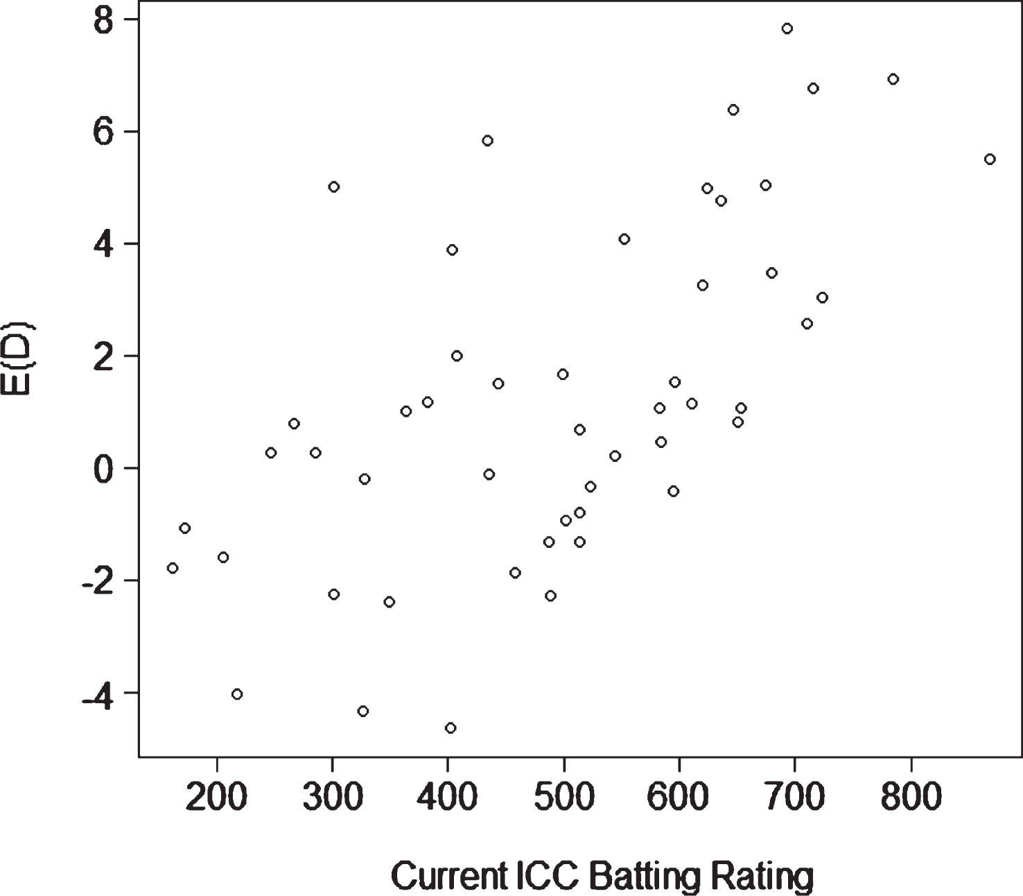
Fig.2
Scatterplot of E (D) (current form) against the Reliance ICC rating for bowlers.
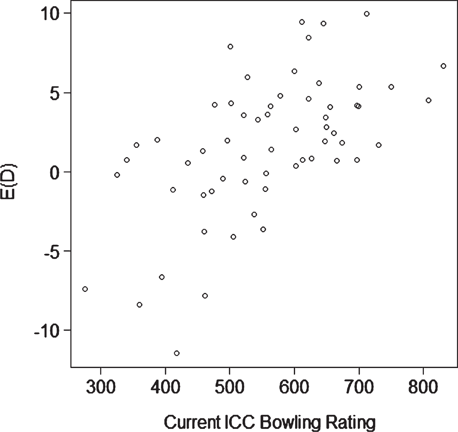
Fig.3
Scatterplot of E (D) (current form) against the Reliance ICC rating for all-rounders.
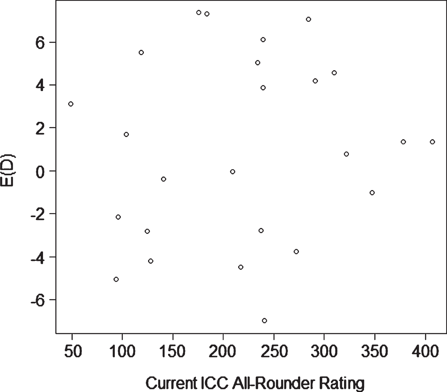
Fig.4
Most recent IPL salary versus current form E (D) for pure batsmen. Triangles represent 2012 salaries, plus signs (+) represent 2013 salaries, and cross signs represent 2014 salaries.
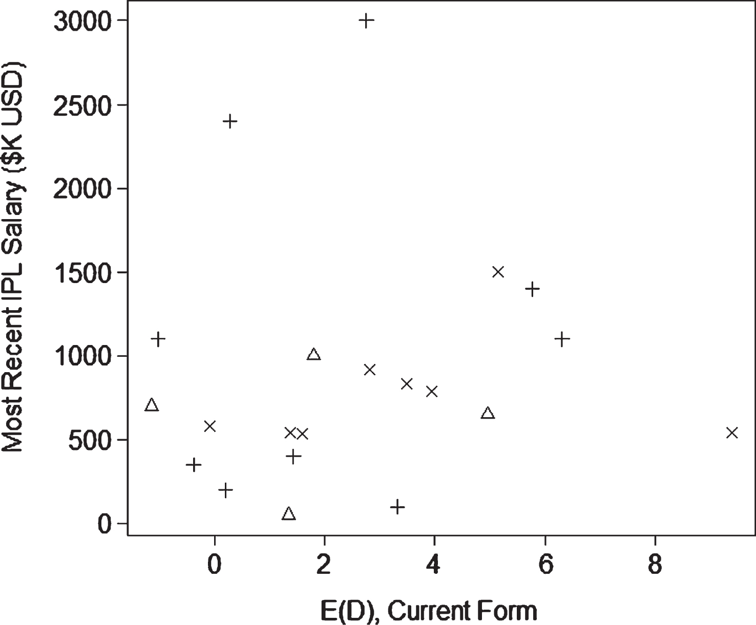
Fig.5
Most recent IPL salary versus current form E (D) for bowlers. Triangles represent 2012 salaries, plus signs (+) represent 2013 salaries, and cross signs represent 2014 salaries.
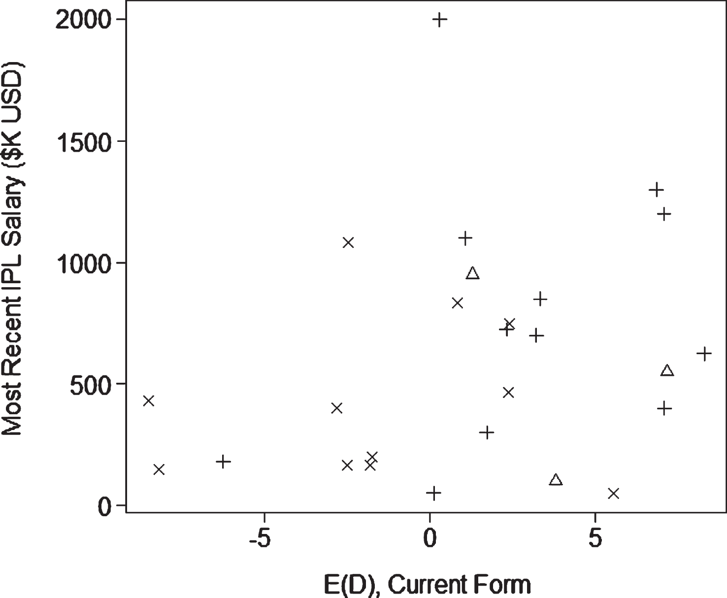
Fig.6
Most recent IPL salary versus current form E (D) for all-rounders. Triangles represent 2012 salaries, plus signs (+) represent 2013 salaries, and cross signs represent 2014 salaries.
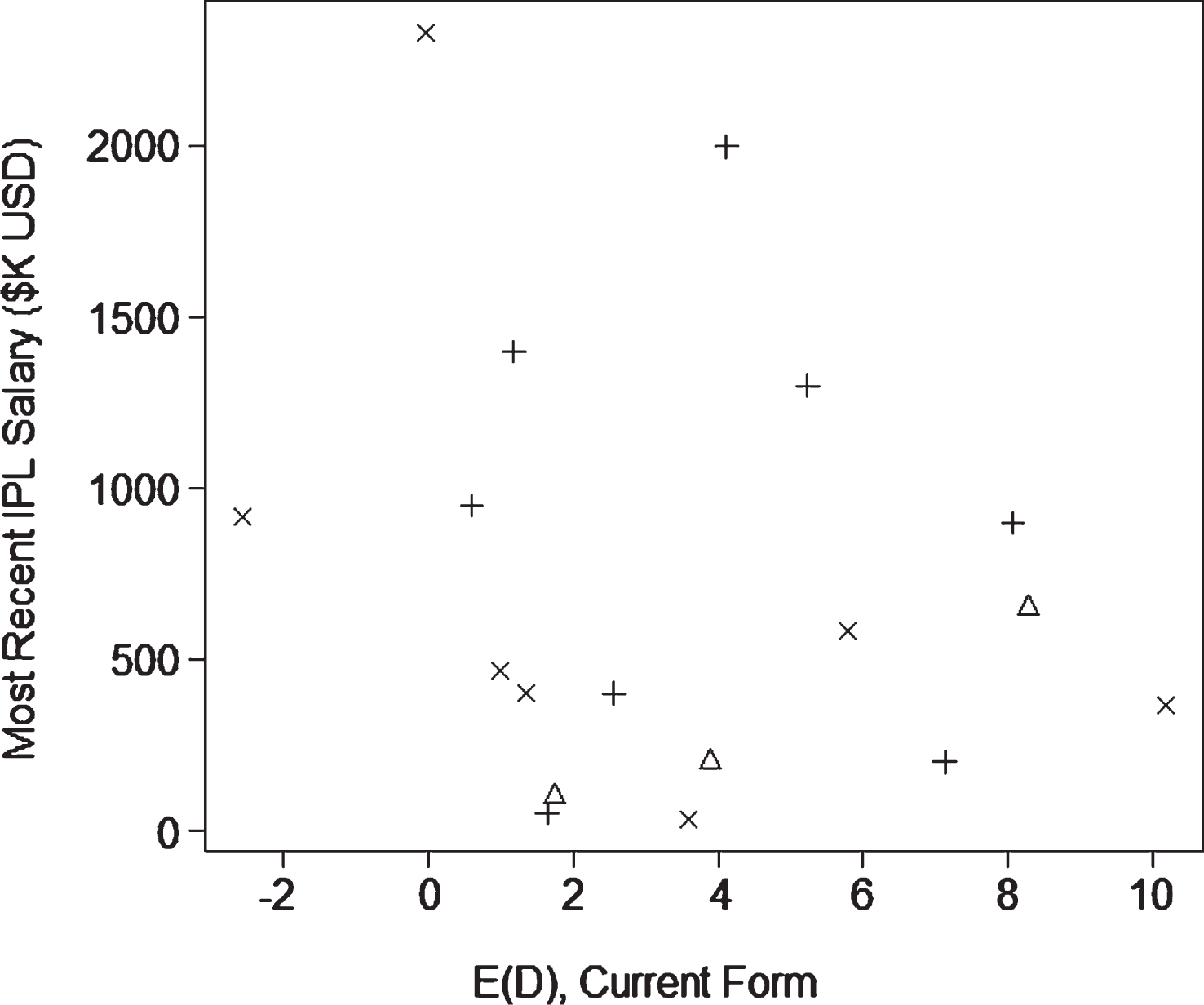
Fig.7
Most recent IPL salary versus ICC Reliance rating for batsmen (top), bowlers (middle) and all-rounders (bottom).
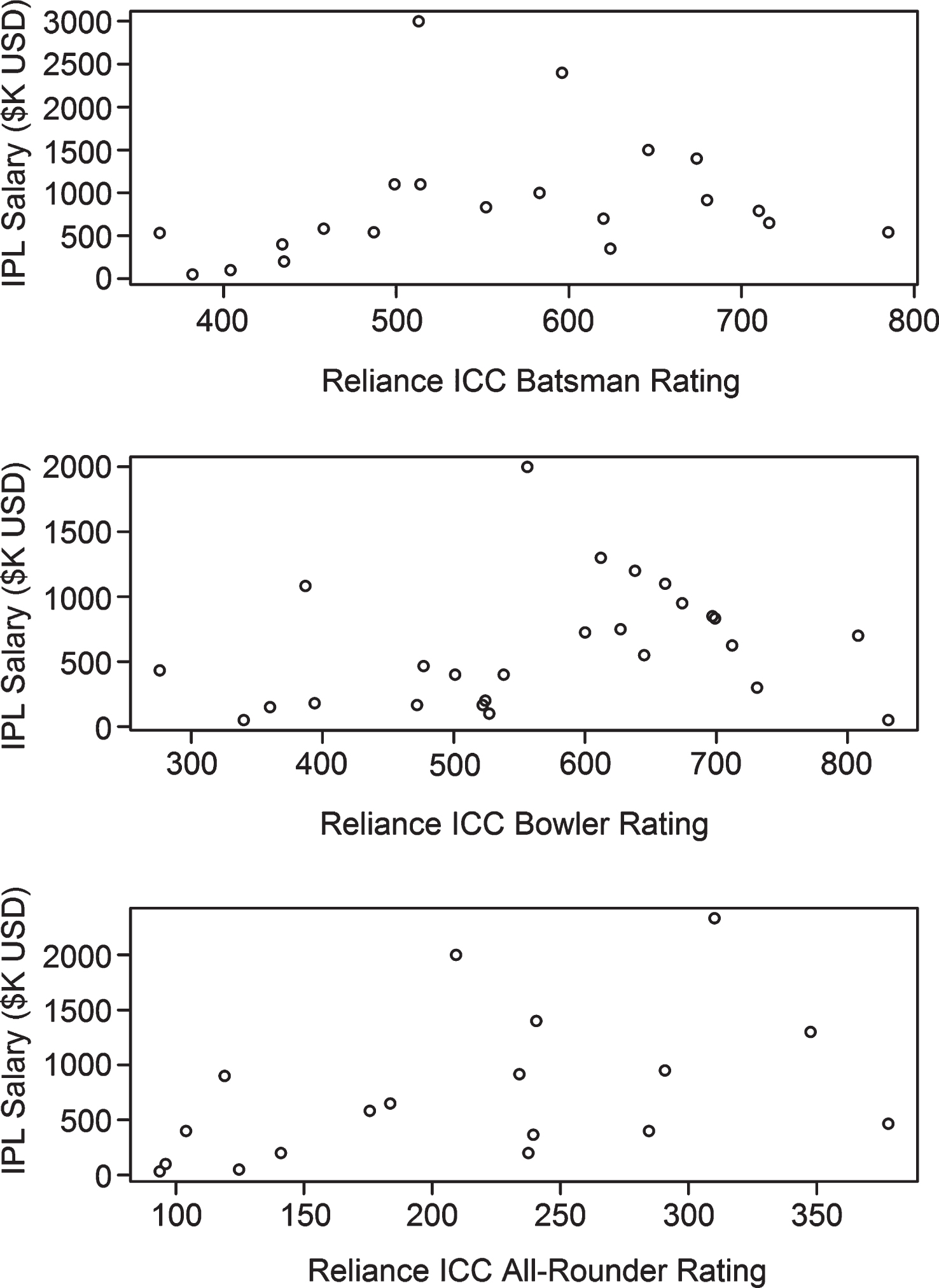
Fig.8
Scatterplot of E (D) using first and second innings data against E (D) using only first innings data.
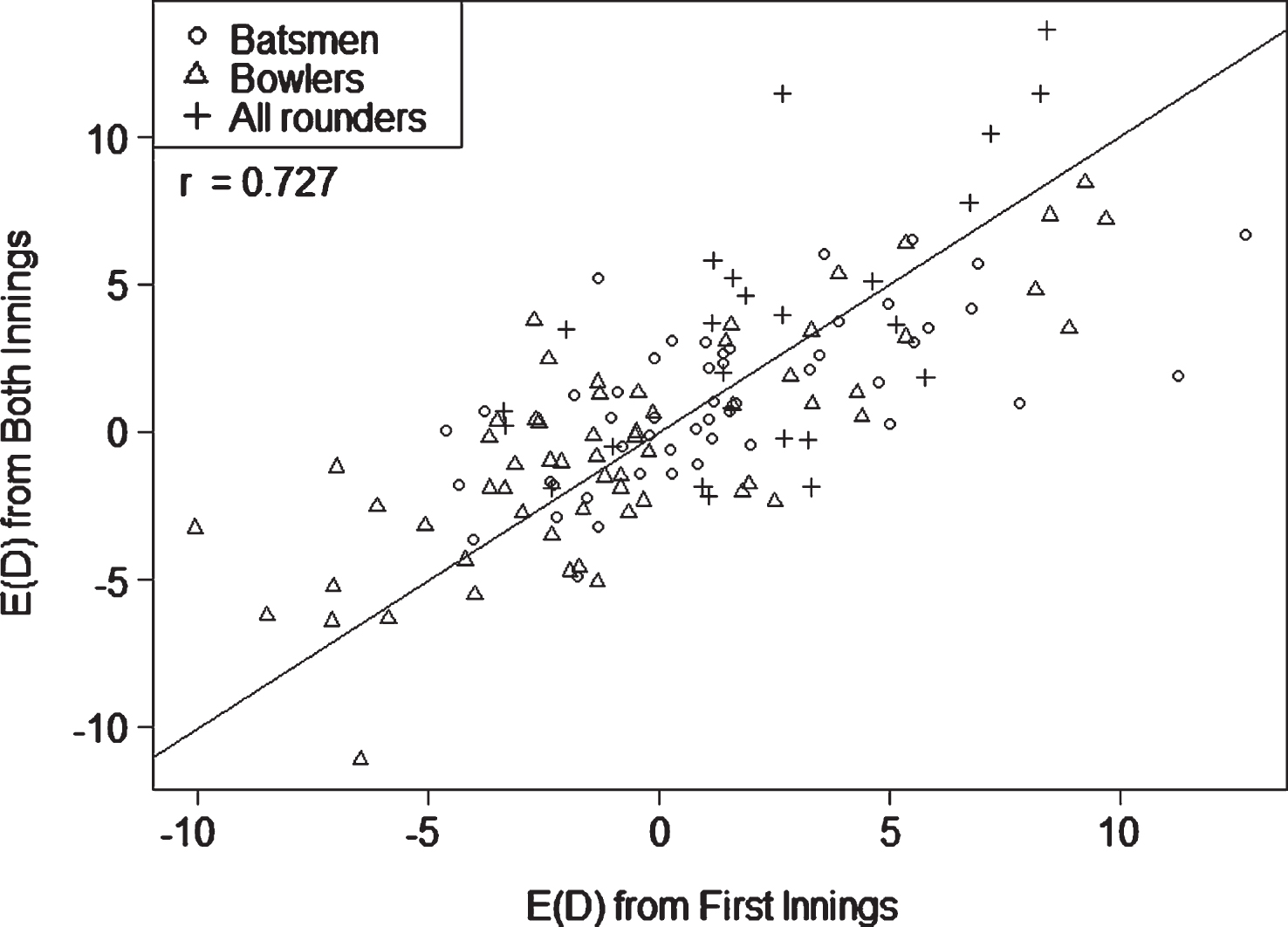
Fig.9
Scatterplot of Croucher’s (2000) statistic for pure batsmen versus E (D).
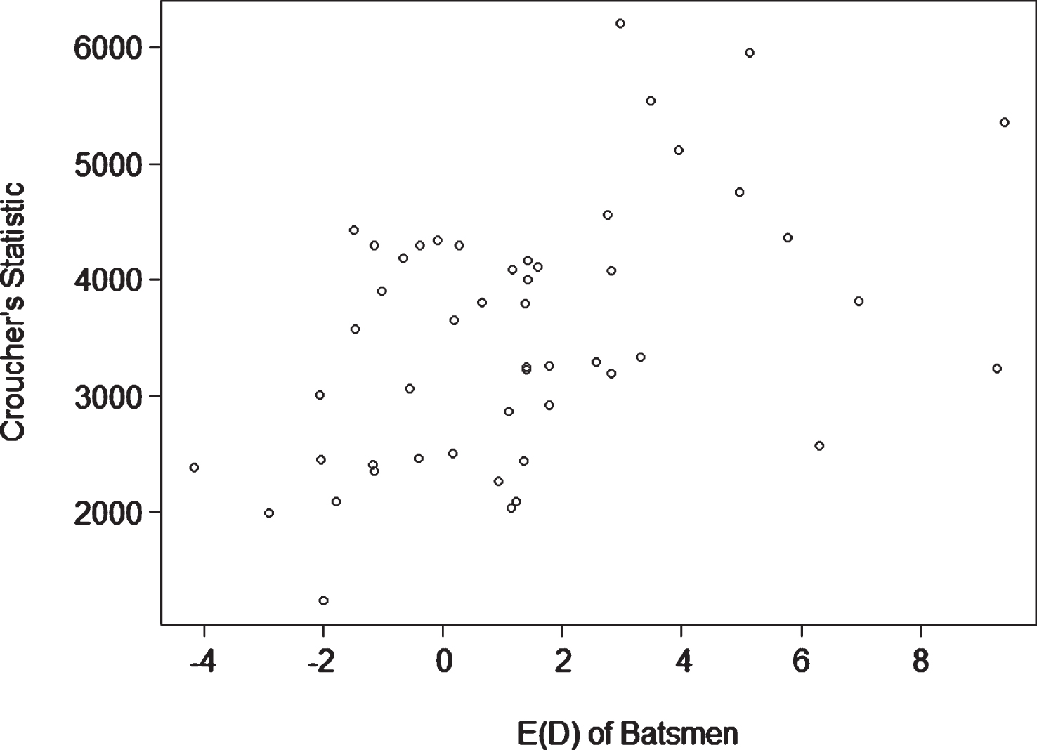
Table 1
Performance metrics of pure batsmen with at least 250 balls faced. Wicketkeepers are marked with an asterisk
| Name | Team | E(D) | Bat Avg | Name | Team | E(D) | Bat Avg |
| A Shehzad | Pak | 7.83 | 25.42 | H Masakadza | Zim | 0.82 | 33.98 |
| BB McCullum* | NZ | 6.93 | 38.25 | C Kapugedera | SL | 0.80 | 20.25 |
| MDKJ Perera | SL | 6.77 | 35.02 | C White | Aus | 0.69 | 29.26 |
| K Pietersen | Eng | 6.40 | 40.78 | B Taylor | Zim | 0.46 | 25.64 |
| R Ponting | Aus | 5.85 | 29.13 | L Thirimanne | SL | 0.29 | 17.86 |
| A Hales | Eng | 5.50 | 42.90 | I Nazir | Pak | 0.27 | 29.23 |
| M Jayawardene | SL | 5.04 | 33.18 | C Kieswetter | Eng | 0.23 | 23.80 |
| Y Khan | Pak | 5.01 | 23.91 | O Shah | Eng | −0.10 | 27.84 |
| E Morgan | Eng | 4.98 | 32.08 | K Akmal | Pak | −0.20 | 19.54 |
| U Akmal | Pak | 4.76 | 30.68 | L Simmons | WI | −0.31 | 29.94 |
| MEK Hussey | Aus | 4.07 | 39.77 | S Butt | Pak | −0.41 | 27.21 |
| D Miller | SA | 3.88 | 24.91 | MS Dhoni* | Ind | −0.78 | 39.03 |
| D Warner | Aus | 3.49 | 29.08 | A Lumb | Eng | −0.92 | 23.48 |
| K Sangakkara* | SL | 3.25 | 35.21 | D Ramdin* | WI | −1.06 | 18.08 |
| G Smith | SA | 3.04 | 32.19 | G Bailey | Aus | −1.31 | 26.31 |
| F du Plessis | SA | 2.58 | 41.64 | Misbah-ul-Haq | Pak | −1.32 | 40.19 |
| N Jamshed | Pak | 1.99 | 21.44 | B Haddin | Aus | −1.58 | 17.92 |
| AB de Villiers | SA | 1.66 | 20.66 | D Chandimal | SL | −1.77 | 12.71 |
| G Gambhir | Ind | 1.53 | 34.33 | Q de Kock* | SA | −1.85 | 35.15 |
| J Buttler | Eng | 1.52 | 23.83 | S Chanderpaul | WI | −2.23 | 20.08 |
| H Gibbs | SA | 1.19 | 18.59 | T Iqbal | Ban | −2.28 | 20.29 |
| H Amla | SA | 1.15 | 26.18 | J Charles | WI | −2.37 | 21.25 |
| R Taylor | NZ | 1.08 | 26.73 | M Boucher* | SA | −4.04 | 19.40 |
| M Guptill | NZ | 1.06 | 32.72 | R Sarwan | WI | −4.33 | 21.83 |
| V Sehwag | Ind | 1.01 | 27.43 | M Rahim* | Ban | −4.64 | 24.29 |
Table 2
Performance metrics of bowlers with at least 250 balls bowled
| Name | Team | E(D) | Econ | Style | Name | Team | E(D) | Econ | Style |
| S Senanayake | SL | 9.94 | 5.72 | Spin | J Botha | SA | 1.84 | 6.51 | Spin |
| H Singh | Ind | 9.43 | 6.50 | Spin | S Tait | Aus | 1.69 | 6.66 | Fast |
| D Vettori | NZ | 9.34 | 5.63 | Spin | J Butler | NZ | 1.68 | 8.12 | Fast |
| I Tahir | SA | 8.44 | 5.57 | Spin | R Price | Zim | 1.38 | 6.47 | Spin |
| B Lee | Aus | 7.88 | 7.46 | Fast | F Edwards | WI | 1.33 | 7.82 | Fast |
| S Badree | WI | 6.66 | 5.72 | Spin | W Parnell | SA | 0.87 | 7.67 | Fast |
| BAW Mendis | SL | 6.34 | 6.65 | Spin | J Anderson | Eng | 0.82 | 7.55 | Fast |
| R Peterson | SA | 5.97 | 7.54 | Spin | R Ashwin | Ind | 0.75 | 7.16 | Spin |
| D Steyn | SA | 5.57 | 6.37 | Fast | R McLaren | SA | 0.74 | 7.46 | Fast |
| G Swann | Eng | 5.34 | 6.45 | Spin | A Razzak | Ban | 0.74 | 7.24 | Spin |
| M Amir | Pak | 5.33 | 7.19 | Fast | D Nannes | Aus | 0.70 | 7.50 | Fast |
| J Taylor | WI | 4.79 | 7.59 | Fast | D Fernando | SL | 0.58 | 7.43 | Fast |
| S Bond | NZ | 4.60 | 7.11 | Fast | S Benn | WI | 0.36 | 7.00 | Spin |
| S Narine | WI | 4.51 | 5.93 | Spin | R Jadeja | Ind | −0.11 | 7.34 | Spin |
| U Gul | Pak | 4.31 | 7.21 | Fast | R Hira | NZ | −0.18 | 7.73 | Spin |
| M Morkel | SA | 4.24 | 7.10 | Fast | Z Khan | Ind | −0.41 | 7.24 | Fast |
| S Ajmal | Pak | 4.17 | 6.41 | Spin | T Southee | NZ | −0.62 | 8.52 | Fast |
| M Starc | Aus | 4.15 | 6.89 | Fast | S Broad | Eng | −1.09 | 7.69 | Fast |
| M Yardy | Eng | 4.11 | 6.38 | Spin | S Akhtar | Pak | −1.14 | 8.36 | Fast |
| N Kulasekara | SL | 4.10 | 7.12 | Fast | M Muralitharan | SL | −1.24 | 6.60 | Spin |
| S Finn | Eng | 3.60 | 7.58 | Fast | T Bresnan | Eng | −1.44 | 7.88 | Fast |
| M McClenaghan | NZ | 3.57 | 8.29 | Fast | IK Pathan | Ind | −2.70 | 7.84 | Fast |
| N Bracken | Aus | 3.43 | 6.93 | Fast | J Dernbach | Eng | −3.64 | 8.35 | Fast |
| S Tanvir | Pak | 3.28 | 7.06 | Fast | K Mills | NZ | −3.77 | 8.22 | Fast |
| NL McCullum | NZ | 2.83 | 6.86 | Spin | J Tredwell | Eng | −4.12 | 8.21 | Spin |
| R Sidebottom | Eng | 2.66 | 7.22 | Fast | B Hogg | Aus | −6.66 | 7.86 | Spin |
| L Malinga | SL | 2.45 | 7.14 | Fast | I Sharma | Ind | −7.38 | 8.69 | Fast |
| M Johnson | Aus | 2.04 | 6.98 | Fast | M Mortaza | Ban | −7.83 | 9.09 | Fast |
| S Pollock | SA | 1.98 | 7.35 | Fast | R Rampaul | WI | −8.37 | 8.45 | Fast |
| P Utseya | Zim | 1.93 | 6.66 | Spin | C Mpofu | Zim | −11.45 | 8.84 | Fast |
Table 3
Performance metrics of all-rounders with at least 250 balls faced and 250 balls bowled
| Name | Team | Style | E (D) Bat | E(D) Bowl | E(D) | BowlEcon | BatAvg |
| A Razzaq | Pak | Fast | 0.30 | 8.25 | 8.55 | 7.39 | 19.75 |
| T Perera | SL | Fast | 7.95 | 0.56 | 8.50 | 8.31 | 34.90 |
| D Sammy | WI | Fast | 2.38 | 5.62 | 7.99 | 7.24 | 18.97 |
| A Mathews | SL | Fast | 2.96 | 3.76 | 6.72 | 6.98 | 26.76 |
| Y Singh | Ind | Spin | 4.98 | 0.39 | 5.37 | 7.46 | 31.39 |
| M Samuels | WI | Spin | 3.43 | 1.19 | 4.62 | 7.78 | 28.59 |
| K Pollard | WI | Spin | 7.00 | −2.50 | 4.50 | 8.11 | 25.47 |
| S Afridi | Pak | Spin | 1.90 | 2.35 | 4.25 | 6.66 | 18.99 |
| C Gayle | WI | Spin | 5.14 | −1.35 | 3.79 | 7.23 | 36.70 |
| S Styris | NZ | Spin | 0.56 | 3.13 | 3.69 | 6.69 | 20.26 |
| J Kallis | SA | Spin | 1.80 | 1.83 | 3.63 | 7.34 | 36.12 |
| DJ Hussey | Aus | Spin | 1.70 | 1.92 | 3.62 | 6.57 | 21.69 |
| JA Morkel | SA | Fast | 2.07 | 1.07 | 3.15 | 7.99 | 23.09 |
| J Franklin | NZ | Fast | −0.37 | 3.26 | 2.88 | 7.46 | 23.06 |
| S Al Hasan | Ban | Spin | −0.85 | 2.91 | 2.06 | 6.57 | 17.58 |
| M Hafeez | Pak | Spin | −0.66 | 2.16 | 1.50 | 6.61 | 21.84 |
| S Watson | Aus | Fast | 1.51 | −0.13 | 1.37 | 7.69 | 26.20 |
| S Malik | Pak | Spin | −1.04 | 2.30 | 1.27 | 6.69 | 23.10 |
| JP Duminy | SA | Spin | 3.58 | −3.28 | 0.29 | 7.62 | 41.87 |
| R Bopara | Eng | Spin | −2.13 | 1.04 | −1.09 | 7.05 | 23.34 |
| J Oram | NZ | Fast | −0.85 | −0.43 | −1.28 | 8.53 | 22.23 |
| DJ Bravo | WI | Fast | 1.79 | −4.10 | −2.31 | 8.49 | 30.68 |
| L Wright | Eng | Spin | −1.04 | −1.88 | −2.93 | 8.21 | 14.51 |
| M Mahmudullah | Ban | Fast | −1.05 | −2.21 | −3.26 | 7.78 | 24.81 |
| S Jayasuriya | SL | Spin | −1.28 | −3.06 | −4.34 | 7.56 | 20.32 |
Table 4
Pearson correlation between E (D) and four established performance metrics: batting average, strike rate (SR), bowling average and economy rate
| Batting E(D) | Bowling E(D) | Bat Avg | Bowl Avg | |||
| vs Bat Avg | vs SR | vs Bowl Avg | vs Econ | vs SR | vs Econ | |
| Batsmen | 0.497 | 0.569 | 0.424 | |||
| All-Rounders | 0.621 | 0.645 | 0.439 | 0.549 | 0.111 | 0.461 |
| Bowlers | 0.714 | 0.773 | 0.543 | |||
Table 5
Comparison of career average and current form characteristics for selected players where the final column denotes the expected number of runs per over
| Role | Name | Form | p i700 | p i701 | p i702-3 | p i704 | p i706 | p i70w | E(R)/Over |
| Batting | AB de Villiers | Career | 0.305 | 0.389 | 0.109 | 0.136 | 0.028 | 0.033 | 7.97 |
| Current | 0.294 | 0.367 | 0.099 | 0.176 | 0.036 | 0.029 | 8.96 | ||
| M Hafeez | Career | 0.368 | 0.365 | 0.091 | 0.113 | 0.027 | 0.037 | 7.02 | |
| Current | 0.343 | 0.373 | 0.109 | 0.107 | 0.032 | 0.037 | 7.31 | ||
| Bowling | U Gul | Career | 0.400 | 0.322 | 0.098 | 0.117 | 0.022 | 0.041 | 6.78 |
| Current | 0.340 | 0.306 | 0.127 | 0.153 | 0.037 | 0.037 | 8.44 | ||
| M Hafeez | Career | 0.349 | 0.422 | 0.084 | 0.090 | 0.029 | 0.026 | 6.86 | |
| Current | 0.351 | 0.422 | 0.081 | 0.094 | 0.029 | 0.023 | 6.78 |

