
Beyond runs expectancy
Abstract
George Lindsey was one of the first to present run scoring distributions of teams of Major League Baseball. One drawback of Lindsey’s approach is that his calculations represented a situation where the team is average. By use of a multinomial/multilevel modeling approach, we look more carefully how run-scoring distributions vary between teams and how run-scoring is affected by different covariates such as ballpark, pitcher quality, and clutch situations. By use of exchangeable models over ordinal regression coefficients, one gets a better understanding which covariates represent meaningful differences between run-scoring of teams.
1Introduction
1.1George Lindsey and the runs expectancy matrix
One the pioneers in sabermetics was George Lindsey, a defense consultant in Canada who had a great love for baseball. Lindsey wrote two remarkable papers in the 1960’s that had a great influence on the quantitative analysis of baseball. In particular, Lindsey (1963) focused on several questions of baseball strategy such as stealing a base, sacrificing to sacrifice a runner to second base, and issuing an intentional walk. Lindsay observed that these questions could be answered by the collection of appropriate data.
“By collecting statistics from a large number of baseball games it should be possible to examine the probability distributions of the number of runs resulting from these various situations. Object of all choices is... to maximize the probability... of winning the game.”
Lindsay noted that the probability of winning at a point during the game depends on the current score and inning and presented tables of W (I, Hi), the probability a team with a lead of I runs at the home half of the ith inning Hi will win the game.
In this paper, Lindsey also considered the runs scoring distribution of a team during an inning. He focused on the run potential, the number of runs a team will score in the remainder of the inning. He noted that the run potential depends on the current number of outs and the runners on base. Since there are three possible number of outs and eight possible runner configurations, there are 3 × 8 = 24 possible out/runner situations, and Lindsey focused on computing
To learn about run potential, Lindsey’s father collected run-scoring data for over 6000 half-innings in games during the 1959 and 1960 seasons, and Lindsey was able to find empirical run-scoring distributions for each of the 24 situations. By computing the mean runs for each situation, he produced the runs expectancy matrix as displayed in Table 1.
At the beginning of an inning with no outs and bases empty, a team will score, on average, 0.46 runs in the remainder of the inning. In contrast, when the bases are loaded with one out, a team will score 1.64 runs in the rest of the inning.
The runs expectancy table has been illustrated in a number of sabermetrics books such as Thorn et al. (1984), Albert and Bennett (2003), Keri et al. (2007) and Tango et al. (2007) for deciding on proper baseball strategy, for learning about the value of plays, and for evaluating players. For example, Chapter 7 of Albert and Bennett (2003) shows the use of run expectancies in determining the values of singles, doubles, triples, and home runs that leads to use of linear weights to measure batting performances. Chapter 9 of Albert and Bennett (2003) uses the run expectancy table to assess the value of common baseball strategies such as a sacrifice bunt, intentional walk, and stealing a base.
Lindsay (1963) cautioned that the run expectancy table represented the situation where all players were “average”.
“It must be reiterated that these calculations pertain to the mythical situation in which all players are ‘average’. The allowance for the deviation from average performance of the batter at the plate, and those expected to follow him, or of runners on the bases, can be made by a shrewd manager who knows his players.”
Also Lindsey (1963) mentioned the possibility of extending this analysis to run-scoring of teams with non-average players.
“If it were desired to provide a manager with a guide to the advisability of attempting various strategies in different situations, it would be possible to complete calculations of the type outlined here for all stages of the game and scores, pertaining to average players. It would also be possible, although onerous, to compute tables for nonaverage statistics, perhaps based on the past records of the individual players on the team.”
1.2Modeling runs scored in an inning
A related line of research is the use of probability models to represent the number of runs scored in an inning or a game. Fits of basic discrete probability models do not accurately represent actual runs scored in an inning. To demonstrate this claim, the Poisson (λ) and negative binomial (n, p) models were separately fit to all inning runs scored in the 2013 season and the fitted probabilities for these two models and the actual run-scoring distribution are displayed in Table 2. Looking at the table, the Poisson fit underestimates the probability of a scoreless inning. Generally, the Poisson fit understates the actual variability in runs scored. The negative binomial fit is better than the Poisson, but this model overestimates the probability of scoring one run and underestimates the probability of scoring two runs.
Since basic probability models appear inaccurate, more sophisticated models for run scoring have been proposed in the literature. For example, Rosner et al. (1996) represents the probability of scoring x runs in an inning by the sum
1.3Multilevel modeling
Another research theme in modeling of sports data is the use of multilevel or hierarchical models to estimate parameters from several groups. Efron and Morris (1975) illustrate the use of an exchangeable model to estimate true batting averages of 18 players from the 1970 season. Albert (2004, 2006) provide further illustrations of the use of an exchangeable model to estimate a set of true batting rates or pitching rates. These models can be extended to the regression framework. Morris (1983) uses an multilevel regression model to assess if Ty Cobb was ever a true.400 hitter. Albert (2009) uses an exchangeable regression model to simultaneously estimate the true pitching trajectories for a number of pitchers.
1.4Plan of the paper
This paper provides an multilevel modeling framework for understanding run scoring of teams in Major League Baseball, and understanding how team run scoring is affected by several factors, such as ballpark, pitcher quality, and runners in scoring position. The basic multilevel model, described in Section 2.1, simultaneously estimates means from several populations, say the average number of runs scored for 30 MLB teams, when the means are believed to follow a normal curve model with unknown mean and standard deviation.
As in Lindsay’s work, we focus on the number of runs scored in a half-inning. A run scoring distribution for a particular team is represented by a multinomial distribution with underlying probabilities over the classes 0 runs, 1 run, 2 runs, 3 runs, and 4 or more runs. Section 2.2 describes a multilevel model for simultaneously estimating a set of multinomial probability vectors. By using this model to estimate the run scoring distributions for the 30 MLB teams, one obtains “improved” estimates at the teams’ abilities to score runs.
After estimating teams’ scoring distributions, we next explore team situational effects. An ordinal regression model, described in Section 2.3, is a useful method for describing how run-scoring probabilities change as one changes a predictor such the quality of a pitcher. This model can be described in terms of the odds of scoring at least a particular number of runs. It is called a proportional odds model as a change in the predictor will result in the odds of scoring runs being increased by a constant factor. Section 3.2 introduces the use of odds in comparing run scoring distributions of the National and American Leagues. Section 3.3 extends this approach to compare run scoring of the 30 teams and illustrates the value of multilevel modeling.
Section 4 focuses on the effect of the following covariates on team run scoring.
• (Home Effects) Teams generally score more runs at home compared to away games. What is the general size of the home/away effect for scoring runs and how does this effect vary among the teams?
• (Pitcher Effects) Clearly, the pitcher has a significant impact on run-scoring. A strong starting pitcher can neutralize the runs scored by even the best-scoring team in baseball. Generally, one expects that a team’s run scoring is negatively associated with the quality of the pitcher. How can one quantify this pitcher effect, and how does this effect differ among teams?
• (Runner Advancement) Run scoring can be viewed as a two-step process – batters get on base and then other batters advance them to home. Do teams differ in their ability to get runners home?
2Methods
2.1Estimating a group of means
Consider the problem of estimating a collection of means from several populations. One observes sample means y1, . . . , yN, where the sample mean from the jth population, yj is distributed normal with mean θj and known standard error σj. We describe this situation in a baseball setting, where N = 30, y1, . . . , y30 correspond to the sample mean numbers of runs scored in a half-inning for the thirty teams for a season, and θ1, . . . , θN are the corresponding population means of runs scored.
One can obtain obtained improved estimates at the population means by means of the following multilevel model. We assume that the means θ1, . . . , θ30 represent a sample from a normal curve with mean μ and standard deviation τ. The locations of the normal curve parameters μ and τ are unknown, and so (under a Bayesian framework) vague or imprecise prior distributions are assigned to these parameters.
One can fit this multilevel model from the observed sample means of runs scored for the 30 teams. In particular, we estimate the population mean and standard deviation μ and τ by
Three sets of estimates
There are three types of estimates of the population means. If we estimate each population mean only by using data from the corresponding sample, we obtain individual estimates
By use of the multilevel model, we obtain improved estimates of the population means that compromise between the individual and combined estimates. The multilevel (ML) estimate of the population mean for team j,
2.1.1Example
This multilevel model was fit to the sample means of runs scored for the 30 teams in the 2013 season. We obtain the estimates
2.2Estimating collections of multinomial data
A related problem is estimating a multinomial population. Suppose we classify data into k bins and observe the vector of frequencies W = (w1, . . . , wk). The vector W is assumed to have a multinomial distribution with sample size N = w1 + . . . + wk and probability vector p = (p1, . . . , pk), where pj represents the probability that an observation falls in the jth bin. In our setting, we classify the number of runs scored in an inning in the five bins 0, 1, 2, 3, and 4 or more runs, and the frequencies w1, . . . , w5 represent the number of innings where a particular team scores the different number of runs.
This type of multinomial data on runs scored is collected for each of the 30 baseball teams. Let W 1, . . . , W 30 denote the vectors of frequencies of runs scored for the 30 teams. We assume the vector for the jth team W j is multinomial with probability vector p j . We are interested in estimating the probability vectors p 1, . . . , p 30. As in the population means case, we can consider individual, combined, and multilevel estimates for the probability vectors.
Individual estimates
Suppose we use the data from only the jth team to learn about its run scoring tendencies. Then the probabilities of falling in the different run groups are estimated by the individual estimates:
Combined estimates
Instead, suppose we assume that the probabilities of falling in the different runs group are the same for all teams; that is, p 1 = . . . = p 30. Then we can estimate each team’s probability vector by the combined estimate
Multilevel estimates
We wish to get improved estimates at the team probability vectors p 1, . . . , p 30 that compromise between the individual estimates and the combined estimates. This is accomplished by means of the following multilevel model. We assume that the unknown probability vectors p 1, . . . , p 30 are a random sample from a Dirichlet distribution with mean vector η and precision K with density proportional to
One fits this multilevel model to the observed count data and one obtains estimates at K and η from the posterior distribution – call these estimates
2.3Groups of ordinal multinomial data with regression
Ordinal logistic regression
Suppose one observes the vector of run frequencies w = (w1, . . . , wk) which is multinomial with probability vector p = (p1, . . . , pk). The categories 1,..., k are ordinal – in our setting, these categories will be “0 runs”, “1 run”, “2 runs”, etc. Define the probability
Suppose one observes a variable x that influences the run-scoring probabilities p. The ordinal logistic model (see McCullagh (1980) and Johnson and Albert (1999)) says that the log of the odds of scoring at least c runs is a linear function of x. This model is written as
Ordinal logistic regression over groups
As a more general set-up, suppose we observe run-scoring frequencies for N = 30 teams, where the frequencies for the jth team w
j
is multinomial with probability vector
One can now use the estimation of separate means methodology of Section 2.1 to get improved (multilevel) estimates at the regression effects. The true regression effects β1, . . . , βN are given a normal distribution with mean μ and standard deviation τ, we place vague priors on μ and τ. Improved estimates are provided by fitting this multilevel model – the estimates have the general form
3League and team differences in scoring
3.1Run scoring of all teams in 2013 season
We begin by collecting in Table 3 the runs scored for all complete innings (three outs) in the 2013 season. Since scoring five or more runs in an inning is relatively rare, Table 4 collapses the data from Table 3 by combining the counts of runs four or greater into the class “4+”.
3.2Logits and comparing scoring of the NL and AL
To motivate our general approach, a useful reexpression of a proportion p is the logit
Logits are useful in comparing groups of ordinal data such as runs scored. To illustrate, suppose we want to compare the runs scored per inning of National and American League teams in the 2013 season. First we obtain the counts of runs scored by the two leagues as displayed in Table 6. Each row of counts of the table is converted to proportions, and then logits are computed using each of the four breakpoints. The logits for each league are displayed in Table 7 and the “Difference” row gives the difference in the logits for the two leagues.
An ordinal regression model is a useful way to summarize the relationship seen in Table 7. If θc is the probability of scoring at least c runs, then the model is
To gain some historical perspective on the run-scoring advantage of the American League, this ordinal regression model was fit for each of the 16 seasons 1998 through 2013. Figure 1 displays a graph of the AL advantage (on the logit scale) against season. It is interesting to note that there is substantial variability in the AL advantage – for example the advantage was 0.121 in 1998 and decreased sharply to 0.019 in 2007. But there is no clear pattern in the changes in AL advantage over this time period. Generally, the probability an AL team scores a large number of runs is about 6% larger than the probability a NL team scores a large number of runs.
3.3Comparing scoring of teams
How does run scoring vary across teams? If we break down this runs table by the batting team in Table 8, we see some interesting variation in runs scored. If one looks at the percentage of big innings (four runs or more), Boston’s percentage of big innings is 3.2, contrasted with Miami’s percentage of 1.4. Boston’s percentage of scoreless innings is 68.9, while the New York Mets were scoreless in 75.8 percent of their innings.
The logit approach described in Section 3 is used to facilitate comparisons in team scoring. Logits were computed for each team using the four breakpoints. For example, for Philadelphia, we computed the four logits
3.4Multilevel modeling of team run distributions
Since there appears to be chance variability in the estimates of run scoring for the individual teams, there may be some advantage to estimating the run scoring distributions simultaneously using a multilevel model. The exchangeable model of Section 2.2 is fit to the run distributions for the 30 teams. The estimate of the smoothing parameter K is 1973. Most teams play close to the median number of innings 1457. So the size of the shrinkage of the individual estimates towards the combined estimate is
4Covariate effects
4.1General method
Section 3 introduced the use of logits in the comparison of run-scoring distributions. To explore the effect of specific covariates like home/away, pitcher quality, and clutch hitting on scoring, we fit the general ordinal logistic model of the form
1. The ordinal logistic model is first fit separately to run-scoring data for each of the 30 teams. One obtains the regression effects
2. The multilevel exchangeable model in Section 2.1 is used to simultaneously estimate the regression effects. We assume the estimated covariate effect
is a compromise between the individual estimate
4.2Home versus away effects
To consider a team’s scoring advantage of playing at home, write the logit of the probability of scoring at least c runs by
This ordinal regression model is initially fit to run-scoring data for all teams in the 2013 season and one obtains the covariate estimate
Since ballparks are known to have a significant impact on scoring, it is natural to fit this home/away model for each of the 30 teams. Figure 4 displays the individual estimates of the parameters β1, . . . , β30 as black dots where the endpoints of the bars correspond to the estimates plus and minus the standard errors. As expected, the individual home/away estimates show substantial variability from the New York Mets (
Next we apply the multilevel model of Section 2.1 to simultaneously estimate the 30 home effects β1, . . . , β30. One obtains the multilevel estimates
4.3Pitcher effects
The same ordinal regression approach can to be used to learn about the pitcher effect on team run-scoring. The logit of the probability of scoring at least c runs in a half-inning is given by
The challenge in this approach is to find a good measure of pitcher quality. Many pitchers are of the relief type with a small number of plate appearances, and the measurements of pitcher quality typically show high variability. We use a multilevel model approach to obtain improved estimates of pitcher quality and these improved estimates are used as covariates in the ordinal model for run scoring.
To begin, we use a run value approach illustrated in Albert and Bennett (2003), Keri et al. (2007) and Tango et al. (2007) to measure the quality of all pitchers who played in the 2013 season. For each plate appearance (PA), we measure the run value as
Figure 5 displays a histogram of the run value measures of the 679 pitchers in the 2013 season. These multilevel estimates shrink the individual mean run value estimates towards the overall value, the degree of shrinkage depending on the number of batters faced. For pitchers who faced fewer than 100 batters, the shrinkage exceeds 80%; for a starter facing 900 batters, the shrinkage was only 35%. In this particular season, Clayton Kershaw stands out with a run value measure of −0.036 – since he faced 934 batters, he saved 934 × -0.036 = -33.6 runs during the 2013 season.
If the ordinal regression model with pitcher quality covariate is fit to data for all teams, one obtains the estimate
By fitting the multilevel ordinal regression model, we learn about the pitcher effects for all 30 teams. Figure 6 displays individual (team) effects by black bars and the multilevel model estimates are displayed by red bars. The individual estimates show substantial variation. For example, Seattle’s regression coefficient is
4.4Advancing baserunners home (clutch effects)
Run scoring generally is viewed as a two-step process. A team places runners on bases and then these runners are advanced to home. There is a special focus in the media on advancing runners who are in scoring position (on second and third base). One commonly hears about the number of runners left on base and the proportion of runners in scoring position who score. Do teams really differ in their abilities to advance runners from scoring position?
To address this clutch hitting question, an ordinal regression model is constructed. For each half-inning, one records the total number of (unique) runners SP who are in scoring position (either on second or third base) and the number of these runners R who eventually score. (Note that R can be smaller than the number of runs that score in the half-inning since runners who score don’t need to be in scoring position.) As before, we classify R into the categories 0, 1, 2, 3, and “4 or more”, and consider the ordinal regression model
To see how this clutch hitting statistic varies between teams, this ordinal regression model was fit separately for all teams. Anaheim and the New York Mets had the smallest and largest regression estimates of
5Multiple regression approach
5.1Introduction
In our exploration of the effects of covariates on run-scoring, we focused on the application of an ordinal regression model with a single covariate. This was done since it is simpler to describe the covariate effects and the shrinkage behavior of the multilevel model. A natural extension of this approach is to model run-scoring of all teams by a large ordinal regression model where one includes all covariates that one believes have an impact on run scoring. Using our general notation, one can write the ordinal logistic model as
where
5.2Example
To illustrate this multiple regression approach, suppose we are interested in learning about the home and inning effects on team run scoring. For the jth team, we write the ordinal regression model as
This model was fit on the 2013 season data. One can represent an estimate of the pair (βj1, βj2) by an ellipse that contains the unknown pair of parameters with 95% probability. Figure 8 displays the estimates of the home and inning effects where one uses individual regression models for the 30 teams, and Fig. 9 displays estimates of the same effects using the multilevel regression model. Note that there are general tendencies for teams to score more at home and in early innings (the ellipses tend to be located in the upper-right section of the graph), but the locations of the ellipses for the multilevel model estimates tend to be shrunk towards a common estimate.
6What covariates are relevant to run-scoring?
The ordinal regression approach seems advantageous to the expected runs approach for understanding team run-scoring, and we have illustrated the use of several covariates such as home/away, pitcher quality, and ability to advance runners in scoring position. But there needs to be a more careful look at all of the team attributes that affect run-scoring. One believes that this modeling approach can be extended to handle many other covariates.
Home/away affect. The home-away run-scoring effects documented actually have several dimensions. A team scores more in their ball park partly due to physical and weather attributes of their ballpark, but there is evidence to suggest that umpires may favor the home team in the calling of balls and strikes. How much of the home/away effect is due to each factor?
Individual batter effects. This paper has focused on run-scoring of teams. But a team’s batting lineup consists of players who aid run-scoring by their ability to get on-base and other players contribute by advancing runners home by extra-base hits. One typically evaluates the contribution of individual hitters by run value, but these run value calculations are based on league averages. One would speculate that one could get better evaluations of hitter runs contributed by using run distributions individualized for the player’s team.
Base-running effects. As documented in the recent World Series between the Royals and the Giants, runs are often scored by good runner advancement. Several of the runs were set up by a runner on second base who advanced to third on a sacrifice fly. Teams clearly differ with respect to their ability to steal and take the extra base, and one would be interested in measuring the effect of base-running on run scoring for all teams.
Situational effects. Runs are scored within a context of the opposing pitcher and defense, and the inning. The measurement of pitcher quality used here is actually a measurement of picher quality and team defense. How can one isolate the effect of these two effects in run scoring? There is a recent movement to shifting the infielders for specific hitters – what is the value of this shift from the viewpoint of runs? During different innings, teams may have different goals towards run-scoring. In close games, the objective might be to score a single run. In other situations, the goal might be to score multiple runs. Do teams differ with their ability to score a single run?
7Summary and concluding comments
The primary objective of this work is to provide a better understanding of the run-scoring patterns in Major League Baseball. Instead of focusing on the mean number of runs scored in a half-inning, we focus on the probability distribution of runs scored. We are interested in how this run-scoring distribution varies among teams and the effect of various covariates such as the ballpark, pitcher/defense, and “runners in scoring position” situations.
The primary method is ordinal regression of the multinomial run-scoring outcome and the use of multilevel modeling to estimate run-scoring over different groups. One finding is that there are some covariates such as ballpark where there are clear team-specific run-scoring advantages. This is not surprising since it is well-known that Coors Field (home of Colorado Rockies) is very advantagous for run-scoring and other parks such as Citi Field (home of the New York Mets) are more restrictive for scoring runs. But there are other covariates such as advancing runners in scoring position where there are little differences between teams in scoring runs. It should be clarified that we do observe differences in teams’ advancing runners in scoring position, but there is little evidence to suggest that teams have different clutch-hitting abilities. If the media understands this conclusion, then there would be less discussion about teams’ batting performances when runners are in scoring position. The goal of future work to find suitable covariates such as the ones suggested in Section 5.2 that have a significanat impact on run-scoring, and the knowledge of these covariates would be helpful for teams building an offense.
Appendix: Estimating collections of multinomial data using an exchangeable model
In Section 2.2, one observes W
1, . . . , W
30, vectors of runs scored for the 30 teams and one assumes that
One estimates the precision parameter K from its marginal posterior distribution. One can show that the posterior density of (K, η) has the form
One estimates (K, η) by the posterior mode, that is, the value
References
1 | Albert, J., 2004. A batting average: Does it represent ability or luck? Technical Report |
2 | Albert J(2006) Pitching statistics, talent and luck, and the best strikeout seasons of all-timeJournal of Quantitative Analysis in Sports2: 12 |
3 | Albert J(2009) Is Roger Clemens’ WHIP trajectory unusual?Chance22: 2820 |
4 | Albert J, Bennett J(2003) Curve BallSpringer |
5 | Efron B, Morris C(1975) Data analysis using Stein’s estimator and its generalizationsJournal of the American Statistical Association70: 350311319 |
6 | Good IJ(1967) A Bayesian significance test for multinomial distributionsJournal of the Royal Statistical Society. Series B399431 |
7 | Johnson V, Albert J(1999) Ordinal Data ModelingSpringer |
8 | Keri JBaseball Baseball Prospectus(2007) Baseball Between the Numbers: Why Everything You Know About the Game is Wrong,’Basic Books |
9 | Lindsey G(1963) An investigation of strategies in baseballOperations Research11: 4477501 |
10 | McCullagh P(1980) Regression models for ordinal dataJournal of the Royal Statistical Society, Series B42: 2109142 |
11 | Morris C(1983) Parametric empirical Bayes inference: Theory and applicationsJournal of the American Statistical Association78: 3814755 |
12 | Rosner B, Mosteller F, Youtz C(1996) Modeling pitcher performance and the distribution of runs per inning in major league baseballThe American Statistician50: 4352360 |
13 | Simonoff J(1995) Smoothing categorical dataJournal of Statistical Planning and Inference47: 14169 |
14 | Tango T, Lichtman M, Dolphin A(2007) The Book: Playing the Percent-ages in BaseballPotomac Books, Inc |
15 | Thorn, J., Palmer, P., Reuther, D., 1984. The Hidden Game of Baseball: A Revolutionary Approach to Baseball and Its Statistics,’ Doubleday Garden City, New York |
16 | Wollner, K., 2000, An analytic model for per-inning scoring distributions, Baseball Prospectus |
Figures and Tables
Fig.1
American League run-scoring advantage over the National League for the seasons 1998 to 2013, the advantage is the estimate of the parameter β in the fit of the ordinal regression model. A smoothing curve indicates that the American League advantage in scoring runs has remained pretty constant over this time interval.
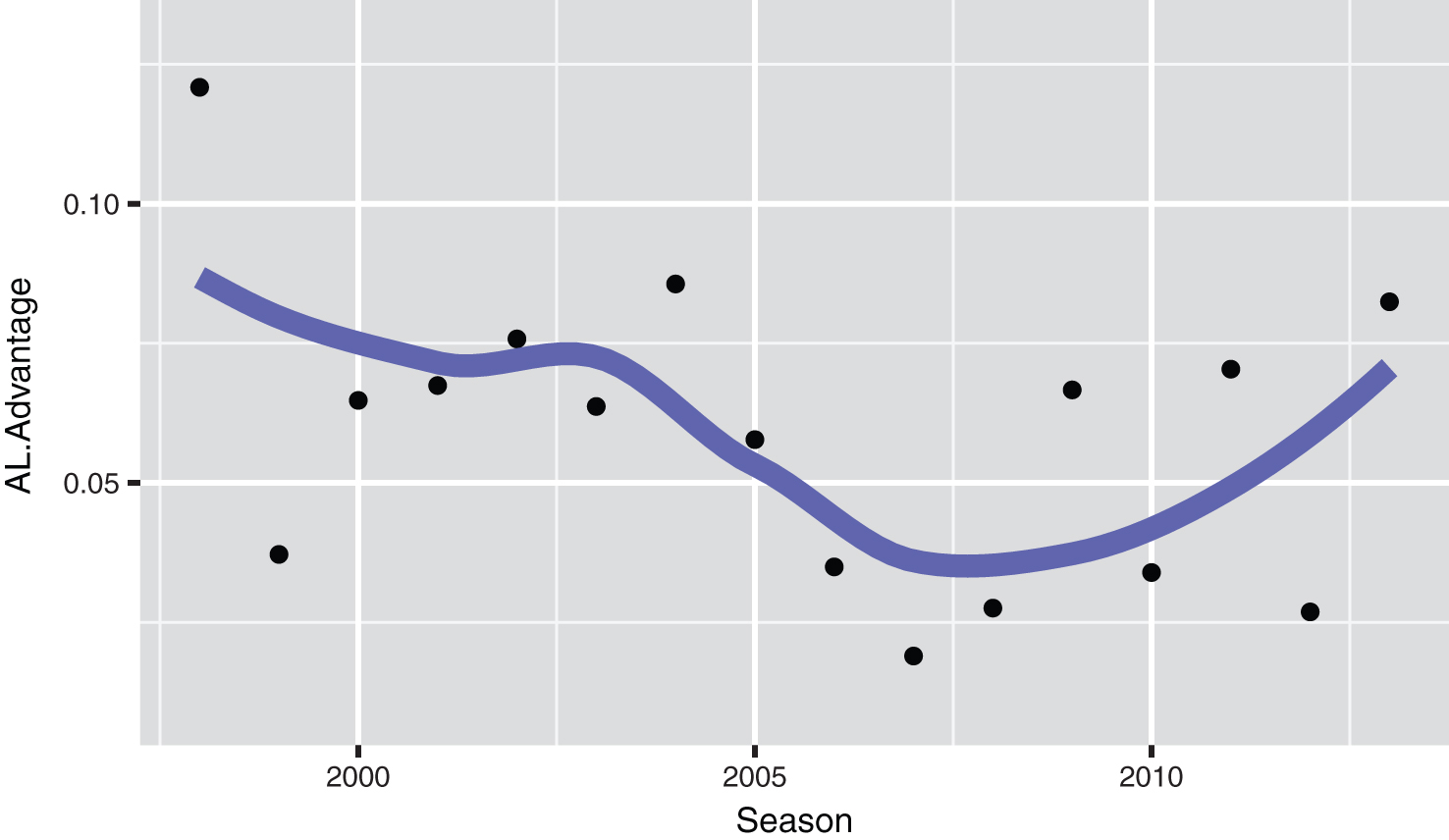
Fig.2
Logit run scoring estimates for all teams. A team’s residual logits were obtained by subtracting the overall logits.
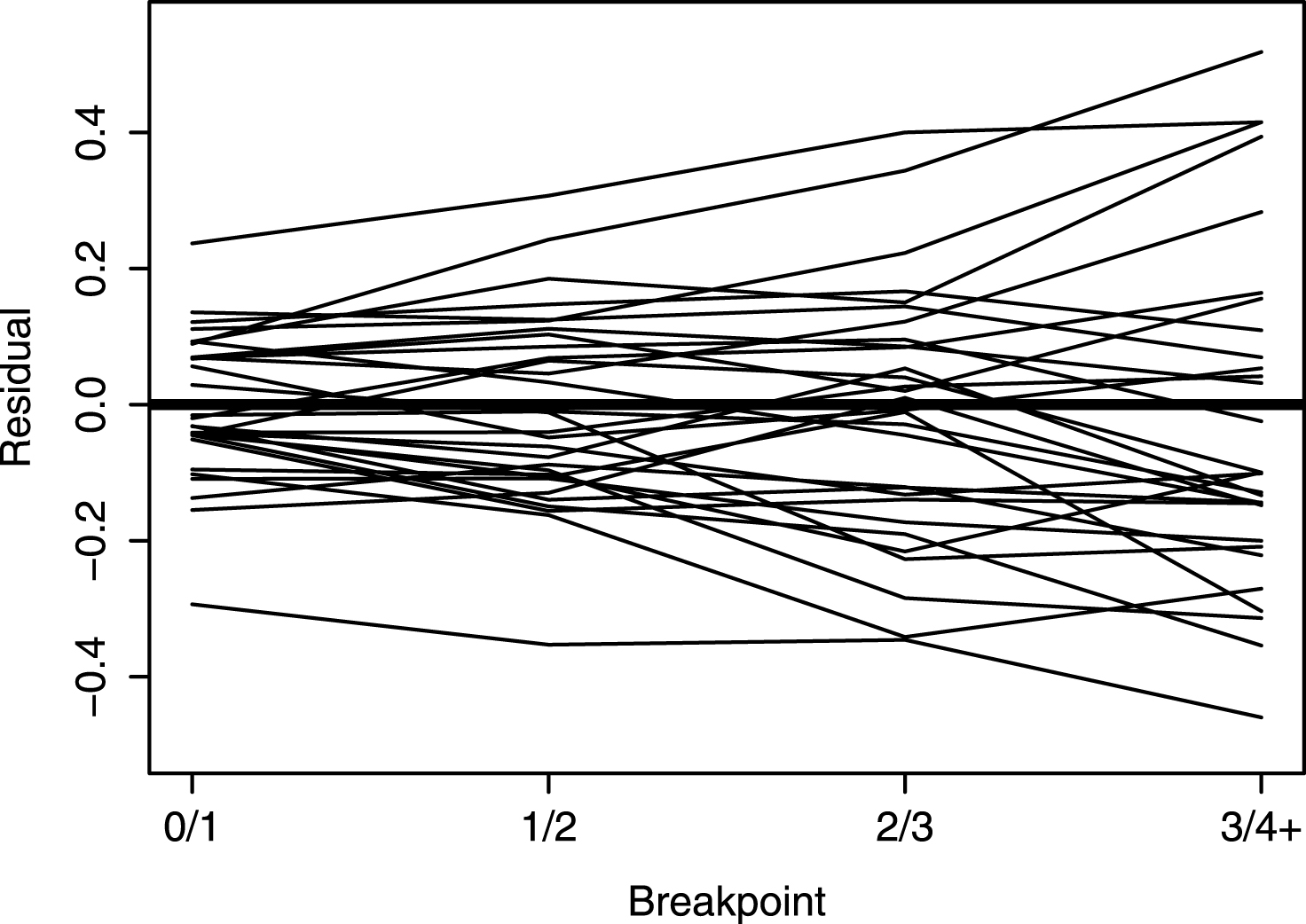
Fig.3
Logit run scoring estimates for all teams using a multilevel model. The residual logits were obtained by subtracting the overall logits.
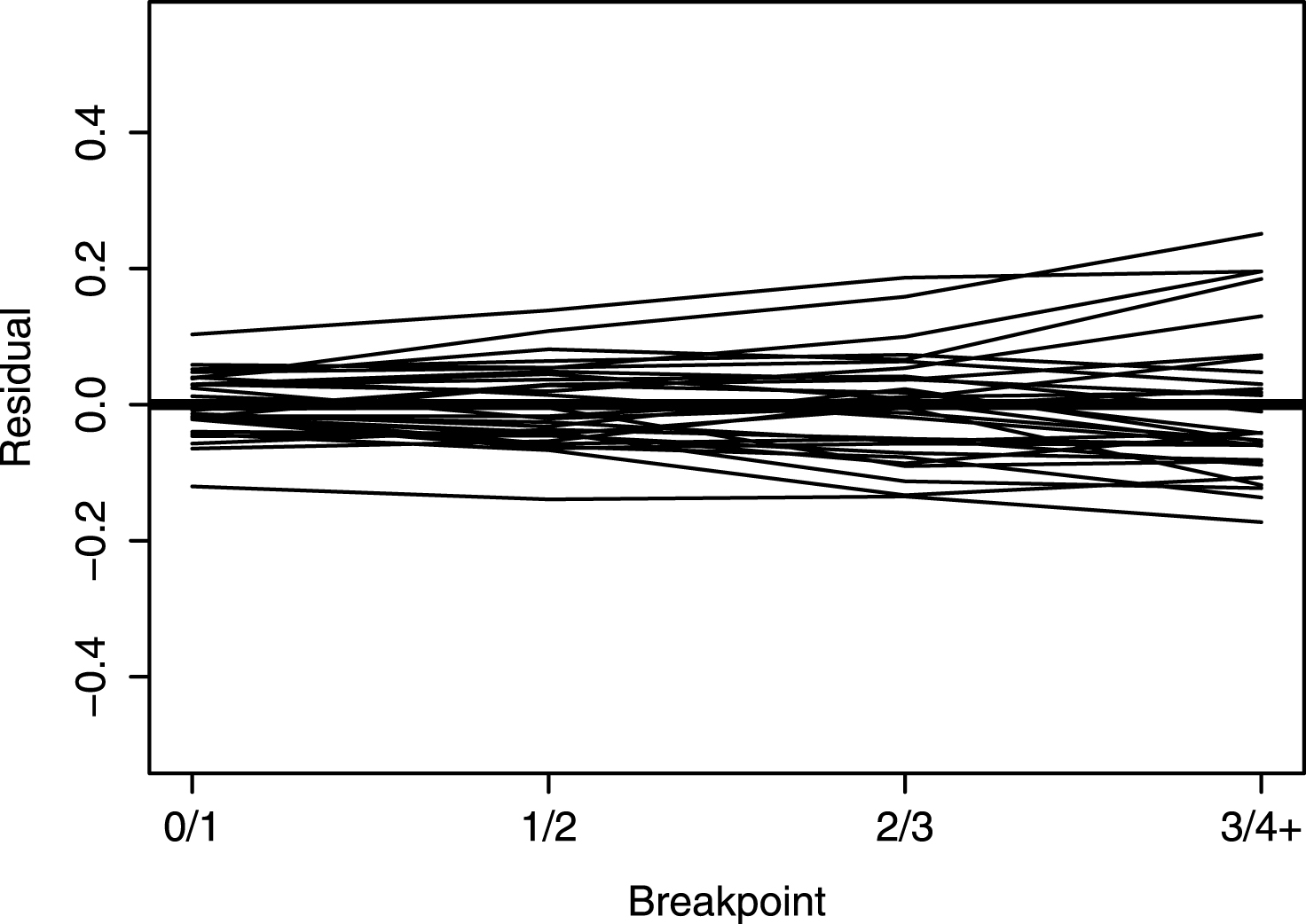
Fig.4
Individual and multilevel home field run effects for all teams. The black line represents the individual estimate plus and minus the standard error and the red line represents the multilevel estimate plus and minus the standard error.
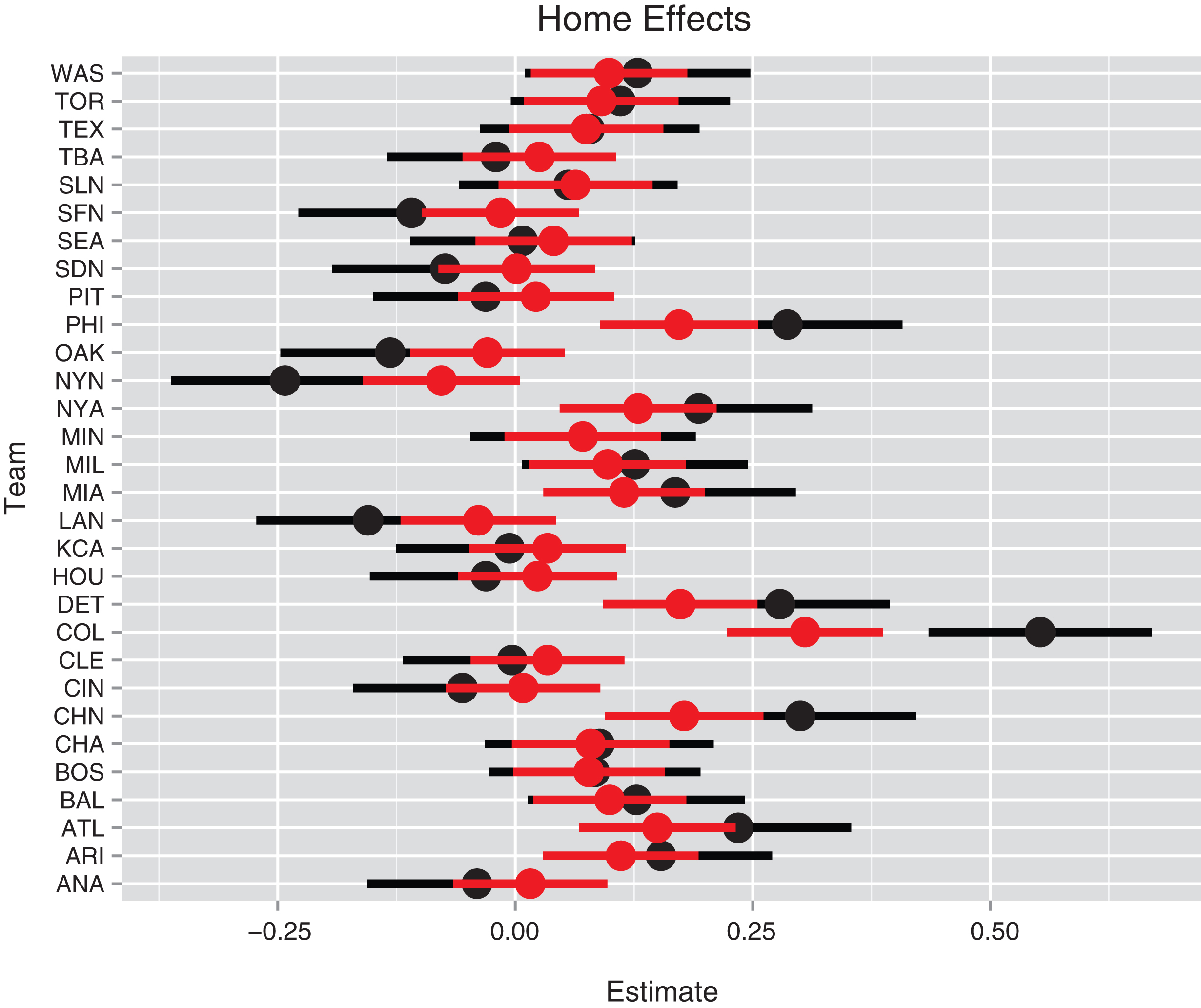
Fig.5
Histogram of abilities of all pitchers in 2013 season.
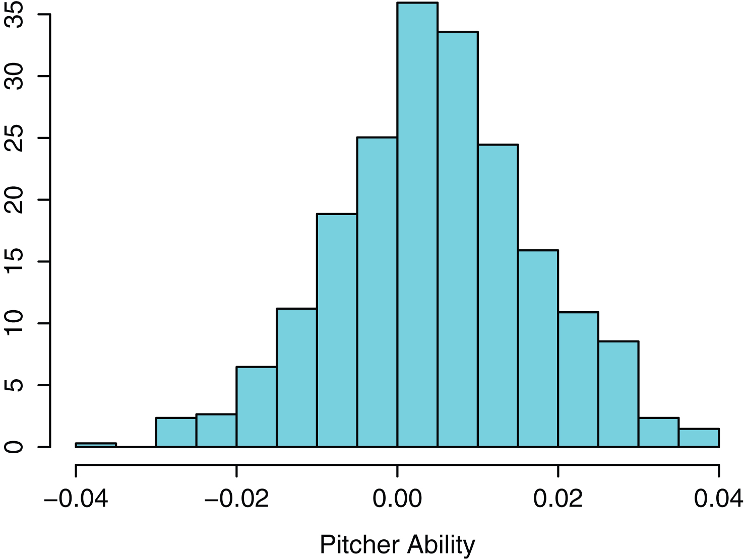
Fig.6
Individual and multilevel pitcher effects for all teams. The black line represents the individual estimate plus and minus the standard error and the red line represents the multilevel estimate plus and minus the standard error.
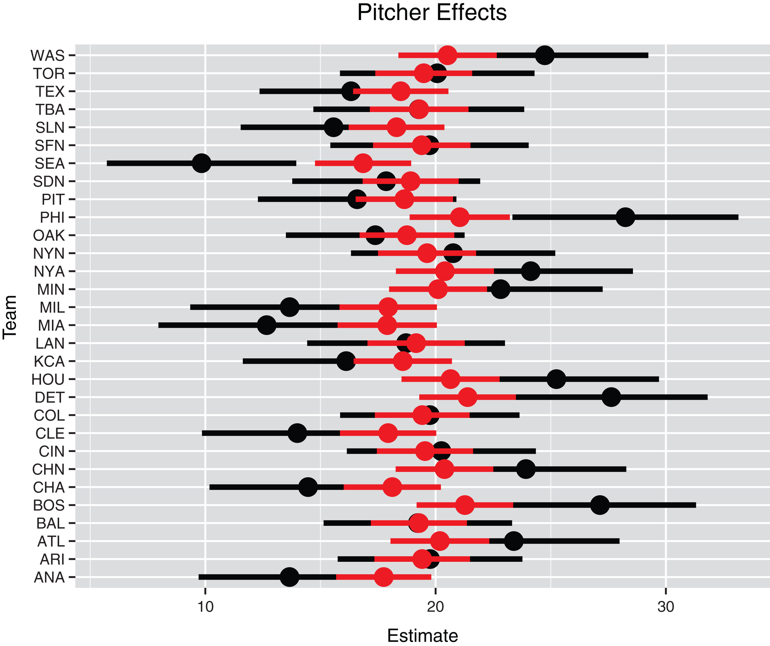
Fig.7
Individual and multilevel clutch effects for all teams. The black line represents the individual estimate plus and minus the standard error and the red line represents the multilevel estimate plus and minus the standard error.
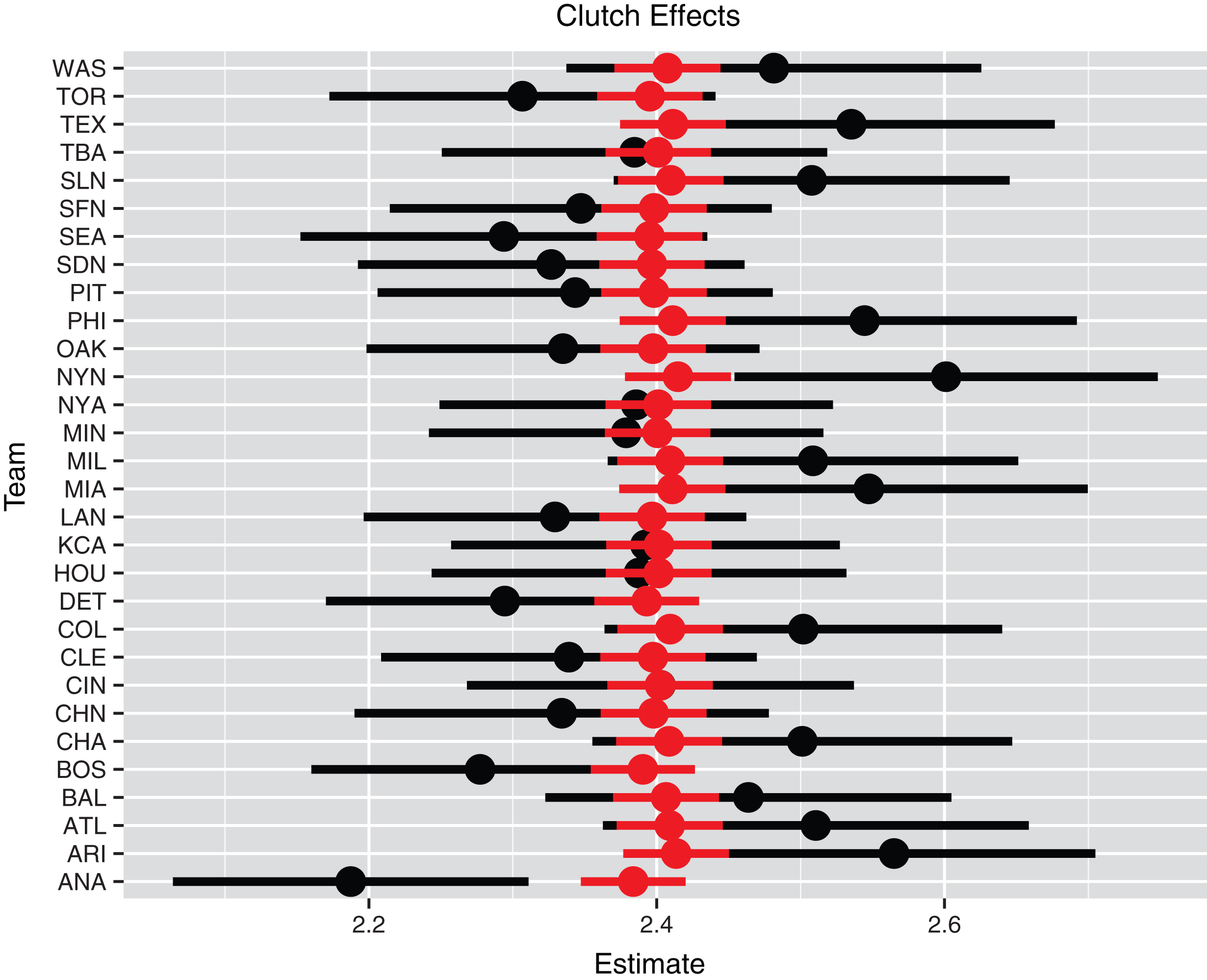
Fig.8
Individual team estimates of home/away and early/late inning effects from ordinal multivariate regression model for 2013 season. Each ellipse represents the location of a 95% confidence region and the region corresponding to Colorado is labelled.
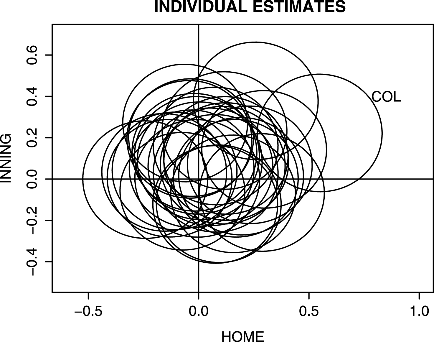
Fig.9
Multilevel ordinal regresssion model estimates of home/away and early/late inning effects for 2013 season. Each ellipse represents the location of a 95% confidence region and the region corresponding to Colorado is labelled.
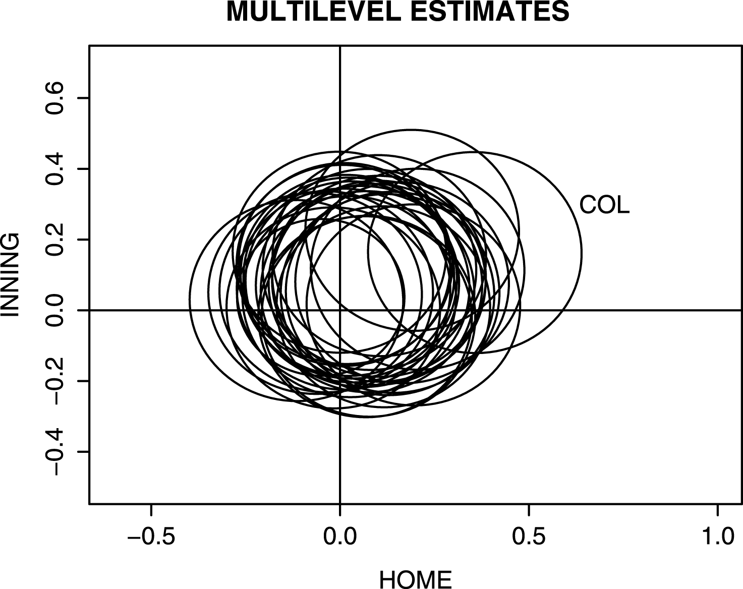
Table 1
Lindsey’s runs expectancy matrix from Lindsey (1963)
| Outs | Bases occupied | |||||||
| 0 | 1 | 2 | 3 | 1,2 | 1,3 | 2,3 | 1,2,3 | |
| 0 Outs | 0.46 | 0.81 | 1.19 | 1.39 | 1.47 | 1.94 | 1.96 | 2.22 |
| 1 Out | 0.24 | 0.50 | 0.67 | 0.98 | 0.94 | 1.12 | 1.56 | 1.64 |
| 2 Outs | 0.10 | 0.22 | 0.30 | 0.36 | 0.40 | 0.53 | 0.69 | 0.82 |
Table 2
Basic probability model fits to runs scored in MLB. The Actual column gives the observed fractions of scoring 0, 1, 2,... runs in the 2013 season and the Poisson and NB columns give the estimated fractions from fitting the Poisson and negative binomial distributions
| Runs | Actual | Poisson λ = 0.462 | NB n = 0.399, p = 0.464 |
| 0 | 0.738 | 0.630 | 0.736 |
| 1 | 0.146 | 0.291 | 0.158 |
| 2 | 0.066 | 0.067 | 0.059 |
| 3 | 0.029 | 0.010 | 0.025 |
| 4 | 0.013 | 0.001 | 0.012 |
| 5 | 0.005 | 0.000 | 0.005 |
| 6 | 0.002 | 0.000 | 0.003 |
| 7 | 0.001 | 0.000 | 0.001 |
Table 3
Frequency table of runs scored for all complete innings in 2013 season
| Runs | Count | Runs | Count |
| 0 | 32315 | 6 | 81 |
| 1 | 6400 | 7 | 38 |
| 2 | 2899 | 8 | 14 |
| 3 | 1254 | 9 | 4 |
| 4 | 584 | 10 | 1 |
| 5 | 207 | 11 | 1 |
Table 4
Counts and percentages of inning runs scored with the new category “4+”
| Runs | 0 | 1 | 2 | 3 | 4+ |
| Count | 32315 | 6400 | 2899 | 1254 | 930 |
| Percentage | 73.80 | 14.60 | 6.60 | 2.90 | 2.10 |
Table 5
Logits of runs scored for all breakpoints
| Breakpoint | 0/1 runs | 1/2 runs | 2/3 runs | 3/4+ runs |
| Proportion scoring “large” runs | 0.262 | 0.116 | 0.050 | 0.021 |
| Proportion scoring “small” runs | 0.738 | 0.884 | 0.950 | 0.979 |
| Logit = | -1.036 | -2.031 | -2.944 | -3.842 |
Table 6
Runs scored per inning by the American and National Leagues in the 2013 season
| Runs | 0 | 1 | 2 | 3 | 4+ |
| American League | 15963 | 3246 | 1497 | 654 | 500 |
| National League | 16352 | 3154 | 1402 | 600 | 430 |
Table 7
Logits of runs scored for all breakpoints for the two leagues
| Breakpoint | 0/1 runs | 1/2 runs | 2/3 runs | 3/4+ runs | Median |
| American League | -0.996 | -1.980 | -2.887 | -3.755 | |
| National League | -1.074 | -2.082 | -3.011 | -3.912 | |
| Difference | 0.078 | 0.102 | 0.124 | 0.157 | 0.113 |
Table 8
Percentages of different inning runs scored for all teams in the 2013 season
| BAT_TEAM | R0 | R1 | R2 | R3 | R4 | |
| 1 | ANA | 72.4 | 15.5 | 6.5 | 2.8 | 2.8 |
| 2 | ARI | 74.6 | 13.1 | 7.1 | 3.3 | 1.9 |
| 3 | ATL | 74.2 | 13.5 | 6.9 | 2.9 | 2.5 |
| 4 | BAL | 71.1 | 16.0 | 7.2 | 3.4 | 2.3 |
| 5 | BOS | 68.9 | 15.9 | 7.9 | 4.1 | 3.2 |
| 6 | CHA | 75.7 | 14.2 | 6.4 | 2.0 | 1.6 |
| 7 | CHN | 76.3 | 12.9 | 6.3 | 2.7 | 1.7 |
| 8 | CIN | 72.7 | 16.2 | 6.2 | 2.7 | 2.2 |
| 9 | CLE | 71.4 | 15.4 | 7.4 | 3.5 | 2.4 |
| 10 | COL | 72.4 | 15.1 | 7.0 | 3.4 | 2.1 |
| 11 | DET | 72.0 | 13.6 | 7.4 | 3.4 | 3.5 |
| 12 | HOU | 76.7 | 13.0 | 5.3 | 3.2 | 1.8 |
| 13 | KCA | 74.4 | 14.0 | 5.6 | 3.4 | 1.9 |
| 14 | LAN | 73.2 | 15.3 | 7.5 | 2.3 | 1.7 |
| 15 | MIA | 79.1 | 12.5 | 4.9 | 2.2 | 1.4 |
| 16 | MIL | 74.6 | 14.4 | 6.6 | 2.5 | 1.9 |
| 17 | MIN | 74.6 | 15.2 | 6.0 | 2.7 | 1.5 |
| 18 | NYA | 74.6 | 14.2 | 6.1 | 2.9 | 2.2 |
| s 19 | NYN | 75.8 | 13.6 | 6.3 | 2.5 | 1.7 |
| 20 | OAK | 72.0 | 14.4 | 7.9 | 2.6 | 3.1 |
| 21 | PHI | 75.6 | 13.8 | 6.5 | 2.1 | 1.9 |
| 22 | PIT | 74.4 | 15.4 | 5.8 | 2.6 | 1.8 |
| 23 | SDN | 74.8 | 15.1 | 5.7 | 2.5 | 1.8 |
| 24 | SEA | 74.6 | 14.7 | 6.9 | 2.2 | 1.6 |
| 25 | SFN | 74.6 | 14.9 | 5.6 | 3.4 | 1.6 |
| 26 | SLN | 71.6 | 15.5 | 6.8 | 3.0 | 3.2 |
| 27 | TBA | 71.9 | 16.1 | 7.2 | 2.9 | 1.8 |
| 28 | TEX | 72.5 | 14.8 | 7.6 | 2.6 | 2.5 |
| 29 | TOR | 72.4 | 14.8 | 7.4 | 3.2 | 2.2 |
| 30 | WAS | 74.1 | 14.4 | 6.7 | 3.0 | 1.9 |

