
Generalized trajectory fuzzy clustering based on the multi-objective mixed function
Abstract
Spatio-temporal trajectory clustering can extract behavior and moving pattern of object with the change of time and space by exploring similar trajectories. Most of trajectory clustering method can be achieved by expanding the traditional clustering algorithms. Considering the limitations of fitness and optimization of most clustering algorithms, especially for spatio-temporal trajectory data sets, this paper proposes a trajectory fuzzy clustering method based on multi-objective mixed function, which can simultaneously optimize multiple objective function such as FCM and XB when perform particle swarm optimization method. And we also propose a new coarse-grained DTW based on interpolation point for generalization trajectory data and improvement the performance of measure the similarity between trajectories. The experimental results, which implement on the synthetized trajectory data and real vehicle history data by employing the new clustering algorithm, and clustering validity evaluation and hot spots analysis show that the proposed method, which combines different objective functions with different optimization criteria and particle swarm algorithm, can effectively solve the clustering problem and produce better clustering results than the traditional clustering method.
1Introduction
Clustering analysis is one of the most useful methods for knowledge acquisition, and it is explored to discover potential clusters and interesting distribution pattern. The spatio-temporal trajectory clustering can explore the movement patterns and behavior mode of the moving object by mining the similar trajectories and extracting the characteristic trajectories with the change of spatial and temporal dimension. Compared with the static spatial analysis method, it is advantageous to manage the dynamic object accurately. As the main tool of spatio-temporal data mining, it lays the foundation for the further analysis and decision-making in many fields, such as traffic [12], tourism, geography, and so on.
Most of trajectory clustering method were expanded on the typical algorithm, such as k-mean clustering, hierarchical clustering, density clustering, and so on [2, 18, 22]. Other methods include introducing spatial statistical methods like kernel density estimation method [11]. In order to improve the clustering results of the classical algorithm, the optimization methods such as genetic algorithm and particle swarm optimization [15] are considered. These optimization methods often use the validity measure of single clustering algorithm as the optimal criterion of clustering quality [7]. However, the validity measure of single cluster is rarely employed for the data sets with different characteristics. Especially for spatio-temporal trajectory data whose characteristics are different from the general static data, their clustering results will be effected by data structure themselves, similar criterion and the optimal methods. In many clustering analysis applications, it is different to explore the optimization method according to each specific criterion. And the key issue is to establish the optimal method that can meet the multi-optimal criteria as many as possible. A typical method is to combine multi-single criteria clustering algorithm [19]. For instance, the multi-criteria clustering based on multi-objective genetic algorithm was proposed in social science field [13, 16]. Or the hybrid clustering strategy based on multiple clustering methods wasconsidered [8].
Generally, different clustering algorithms have different advantages and disadvantages, and it will produce clustering results with different quality. The extended research [14] that analyzes and compares different clustering methods shows that there is no common clustering strategy, which can solve the problems in different application fields. It is important for clustering analysis to take account of multi-optimal criteria, and we propose a clustering strategy named “mixed fuzzy clustering method based on multi-objective function”. The method produces the optimal clustering result by implement the PSO algorithm, which simultaneously optimize two different functions. The strategy mixes two different optimal criterions and performs well when clustering trajectory data.
2Related work
2.1Measure the similarity between spatio-temporal trajectories
The spatio-temporal trajectory is spatial position data set based on time series. Generally, we need to confirm fitting measure function to compare the similarity between two trajectories. Trajectory similarity measure is one of the most key issues during clustering analysis. And most of measure techniques mainly focus on the following:
– The Euclidean distance is one of the most original trajectory similarity measure methods. It is only used to compute pairwise points between two trajectories. When the two trajectories scales are inconsistent, lacking of data points will make that computing Euclidean distance fail to establish. Therefore, there are many limitations when measure trajectory similarity.
– DTW [3] is usually used to calculate the similarity between two sequences. And it is a kind of dynamic programming method for time series similarity measure. Compared with other approaches, it isn’t limited by the length of time series. Given two time series Q and C, which their data lengths are n and m respectively, we can compute the distance between them by DTW. Smaller distance means the higher similarity. The aim of DTW method is to search the minimum total length of the accumulate path which can be achieved by Equation (1). If the point (i, j) is in the optimal path, then the path from point (1, 1) to (i, j) is also locally optimal. DTW can be used to measure distance between trajectories with different series length.
(1)
Other methods like LCSS distance can measure the similarity of the trajectories by obtaining the longest common subsequence between them [20]. In the paper [17], the similarities between trajectories are also computed by sum the minimal distance between two trajectories’ MBBs. And in the method, a trajectory is represented as a list of minimal bounding boxes. Combing the semantic and position similarity, which their proportion can be adjusted by setting weight, can also be employed in trajectory clustering analysis [10].
2.2Particle swarm optimization
Particle swarm optimization (PSO) algorithm is a swarm intelligence computation method, which is proposed by Eberthart and Kennedy in 1995. It can achieve the random search by simulating the social behavior of a flock of birds [7]. In PSO, a flock represents many potential solutions for an optimal problem. And each potential solution is seen as a particle which represents a location in multidimensional space and flies towards its best position and its neighborhood best position at a certain speed. Each particle is seen as an individual consisted of speed and position. On the one hand, the individual has selfness which can judge the position and velocity of the flight according to experience. On the other hand, it also has sociality which adjusts flight speed and position according to the flight of the neighborhood particles. Moreover, the individual constantly seeks a balance between individuality and sociality. The particles’ position can be determined by the following equations during iteration [7].
(2)
(3)
(4)
3Generalized trajectory fuzzy clustering based on multi-objective mixed function
For mixed multi-objective clustering problem [1], searching optimal partitioning can be achieved by implementing on many criteria or objective functions. And each objective function employs own optimization method There may be conflict between them, so we can obtain a set of optimization method instead of single method by optimizing multi-criteria of these objective function.
3.1Multi-objective mixed function optimization
Multi-objective clustering problem [17] can be stated as follows:
In order to automatically optimize the partition result of trajectories, the particle swarm optimization method will be explored which FCM and XB indices need to be optimized simultaneously during clustering process in this paper. FCM algorithm is a clustering method based on the objective function. For a given s dimensional data set X = {X 1, X 2, …, X n }, it is defined as follows [6]:
(5)
As described above (see 2.1), the Euclidean distance is only used to compute pairwise points between two trajectories. While DTW can be used to measure distance between trajectories with different series length, it is an accuracy similarity measure and has good performance in the trajectory clustering analysis [5]. Therefore, we introduce DTW as the similarity measure when implement FCM algorithm. The algorithm complexity of DTW is O (n 2). However, the computing efficiency of the DTW algorithm will slow down when the two time series are very long. The algorithm efficiency can be improved by exploring coarse-grained DTW. In this paper, we propose a new coarse-grained DTW based on interpolation point (DTWBIP). A trajectory can be represented by many polylines. And for each polyline on trajectory, we interpolate a point as the representative point. As shown in Fig. 1, the point q 12 will substitute the point q1 and q2 and involve calculation distance. The length of original trajectory can be dramatically reduced by generalization method.
The Xie-Beni index involves the membership values and the dataset itself. It is a compact and separate fuzzy validity function and defined as follows [21]:
(6)
The equation is explained as the ratio of total compactness to the separation of the fuzzy c-partition. For obtaining compact and well-separated clusters, the small values of v XB are expected. From the Equations (5) and (6), both FCM and XB can achieve the optimal result by minimizing the function. And the numerator of XB indices equal to FCM when m = 2, which can express the compactness within cluster. These conflicts between the two indices balance each other critically and lead to high quality solutions [7].
FCM and XB index need to be optimized (minimized) as the fitness objective function of PSO simultaneously, and trajectory fuzzy clustering problem based on multi-criteria optimal can be described as follows:
(7)
3.2Fuzzy clustering optimization algorithm based on multi-objective mixed function
The new trajectory fuzzy clustering (named FTCBMOF) simultaneously optimize FCM and XB when search the optimal partition by PSO, and the algorithm steps are described as follows:
– Randomly initialize a particle swarm, each particle in the group includes nc cluster centroids.
– For each particle in the particle swarm, compute the membership degree u ij of each trajectory by FCM algorithm according to the cluster centroid represented by the particles.
(8)
– Recalculate the clustering centroid by FCM algorithm.
(9)
– The fitness value of the current particle is computed by exploring the Equation (7) which calculate the optimal (minimum) value of the FCM objective function and the XB index.
– If the fitness value is better than the previous best fitness value, set it as the current value of the particle best position according to the Equation (4), and update the best value of the swarm.
– Update the velocity and position according the Equations (2) and (3) which also represent the cluster centroid.
– Calculate difference between cluster centroid before and after updating. If the minimum error criteria or maximum iterations is not attainted, repeat above steps.
– Output the best position of each particle which also the optimal cluster centroid.
The time complexity of the algorithm mainly includes three sub processes. 1) The time complexity of calculation the membership degree and cluster centroids by FCM is o (n c · n · m 2 · d), where n is the number of trajectory data set including m points, d is dimension and n c is the cluster number. 2) The time complexity of computing XB index is o (n c · n · m 2 · d); 3) The time complexity of updating the velocity and position of particle is o (S · d); Moreover, the first process and second process are nested in the third process. Total time complexity is o (2 · t max · S · n c · n · m 2 · d), where t max is the maximum iteration number.
4Experimental result
In order to verify the efficiency of the new algorithm, we compare it with the FCM algorithm by the clustering experiment implemented on the synthetic trajectory points and real trajectory data set. The synthetic data set produced by the generation algorithm of spatio-temporal trajectory include 100 trajectory points towards north and south respectively. While the real historical trajectory contains the data of 50 trucks in the area around Athens in Greece within 33 days. And the structure of each trajectory can be presented as {object-id, trajectory-id, date (dd/ mm/ yyyy), time (hh:mm:ss), latitude, longitude, x, y}. For obtaining the credible experimental results, the parameters of the two algorithm are set to m = 2 and ɛ= 0.00001.
4.1Experimental results of the synthetic data set
The trajectory structure of the synthetic data set represent two direction trajectory set. Given the parameter c = 2, 3, 4, we run the new algorithm and FCM algorithm on the trajectory data set. In order to evaluate their clustering results, the Jaccard coefficient [9] is employed except for XB index. The clustering results can be compared with the structure of data set itself by Jaccard coefficient. And the range of Jaccard coefficient is between 0 and 1. The greater value show that the similarity between partition results and predetermined structure is also higher [9]. The evaluation result between the new algorithm and FCM algorithm are shown in Table 1 when c = 2. From the table, we can see that the XB index of two algorithm are same. But the Jaccard coefficient values are 1 and 0.49 respectively. This shows that the cluster result of new algorithm is coincident with the predetermined structure of data set. While for the partition result generated by FCM, there is not high similarity with the predetermined structure of data set.
Moreover, the XB index value of two algorithm are 0.5 when c = 4. Compared with the result of c = 2, the partition is a suboptimal result. The clustering results produced by two algorithms are shown in Fig. 2, which the results produced by the new algorithm is shown in the left figure and the right figure is the result of FCM. From the right figure, we can see that the cluster generated by FCM is inconsistent with the structure of data set itself. Obviously, three of four clusters both include the data towards north and south. While in left figure, each of cluster produced by the new algorithm only include the data towards one direction. Its partition result is better than the result produced by FCM.
4.2Experimental results of real vehicle historical trajectory
4.2.1Clustering result and validity evaluation
The real trajectory data set mainly consists of six clusters [4]. The number of c in experiments is set to 2, 3, 4, 5, 6 to observe the experimental results because the fuzzy clustering algorithm is a non-supervised classification method. In order to verify the validity of new algorithm, we adopt the XB index, which the smaller value shows the clustering results are better, to test the clustering validity. The results of validity evaluation between new algorithm and FCM algorithm are shown in Table 2. From the table, the minimum value of XB index of the new algorithm is obtained when C = 6. While the minimum value of XB index of FCM algorithm is produced when C = 2. The optimal clustering results generated by the new algorithm are also six cluster as shown in Fig. 3. And each color trajectory represent each cluster in the figure.
4.2.2Hot spot analysis
From the Fig. 3, we can find some obvious local “hot spot”, such as in C4, C5 and C6. The cluster C5, C4 and C6 contain trajectories of 15 trucks, 7 trucks and 4 trucks respectively. And all the trucks passed the “hot spot” area. We can also compare the new algorithm and FCM algorithm by hot spot analysis. The hot spots in each cluster can be produced by kernel density estimation. And the generated results are shown in Fig. 4 by the new algorithm. From the figure, we can find three obvious local “hot spot” area (black shaded area in the figure). The hot spot area in the cluster C1 locate around the Kenteric street of Acharnes city in Greece. While the hot spot area in the clusters C2 and C3 are situated in the area around the first highway section of Agios Stefanos in Greece. And the hot spots area in the clusters C4, C5 and C6 are located near the intersection of Attiki Odos and Periferiaki Lmittou avenue of Pallini in Greece.
The hot spots of each cluster generated by FCM algorithm are shown in Figs. 5 to 6. From the Fig. 6, we can find two hot spots which are located in the area around the first highway section of Agios Stefanos and near the intersection of Attiki Odos and Periferiaki Lmittou avenue of Pallini in Greece respectively. While the cluster C2 only includes two trajectories, and its hot spot is located in the area around the first highway section of Agios Stefanos. The results of hot spots produced by kernel density estimation show that the partition result c = 2 generated by FCM algorithm are not appropriate. And it can not partition the original trajectory data set effectively.
From the experiments performed on the synthetic data, which we already know the data structure, and the real vehicle trajectories with unknown structure, we can see that the clustering results produced by the proposed new algorithm are better than the clustering result generated by the traditional clustering algorithm FCM.
5Conclusion
The trajectory clustering can extract the similar and abnormal features from the spatio-temporal trajectory and find the meaningful patterns by expanding and optimizing the traditional clustering methods. However, most clustering methods will produce different clustering results for the data set with different features. And the method based on single optimal criterion can’t be well fit to the trajectory clustering. Considering the issues, the trajectory fuzzy clustering method based on multi-criteria is proposed in this paper. Our work includes the following: 1) Give the problem description of the new method, and the new method combine the optimal criteria of FCM and XB index and can find the optimal partition when the two function obtain the minimum value simultaneously. 2) Propose a new coarse-grained DTW based on interpolation point (DTWBIP) which can improve the calculation efficiency and give the new clustering algorithm. 3) Perform the new algorithm on the synthetic data and real trajectory for verifying its validity. The experimental results of clustering validity evaluation and hot spot analysis show that the new algorithm can produced better clustering results compared with the FCM algorithm.
Future research will start from the following aspects. 1) The algorithm performance. How to achieve the high performance trajectory clustering analysis is the key issue for big trajectory data. 2) How to apply the clustering analysis to the specific field and make decision support is also hot issue in the research of trajectory clustering.
Acknowledgments
This research was supported by research project of National Natural Science Foundation under Grant 41401452 and 91224008.
References
1 | Ferligoj A, Batagelj V (1992) Direct multicriteria clustering algorithm J Classif 9: 43 61 |
2 | Liu B, De Souza Erico N (2014) Matwin Stan and Sydow Marcin, Knowledge-based clustering of ship trajectories using density-based approach 2014 IEEE International Conference on Big Data 603 608 Washington, DC, United States |
3 | Berndt DJ, Clifford J (1996) Advances in Knowledge Discovery and Data Mining, American Association for Artificial Intelligence Menlo Park 229 248 CA, USA |
4 | Masciari E (2009) A framework for trajectory clustering Lecture Notes in Computer Science 5659: 102 111 |
5 | de Vries GKD, van Someren M (2014) An analysis of alignment and integral based kernels for machine learning from vessel trajectories Expert Systems with Applications 41: 7596 7607 |
6 | Bezdek JC (1981) Pattern Recognition with Fuzzy Objective Function Algorithms New York Plenum Press |
7 | Bocci L, Mingo I (2012) Studies in Theoretical and Applied Statistics 3 12 Berlin Heidelberg Springer |
8 | Lebart L, Morineau A, Piron M (2004) Statistique Exploratoire Multidimensionnelle Dunod, Paris |
9 | Deng M, Liu Q, Li GQ (2011) Spatial Clustering Analysis and Application Science Press Beijing |
10 | Ra M, Lim C, Song YH, Jung J, Kim W-Y (2015) Effective trajectory similarity measure for moving objects in real-world scene Lecture Notes in Electrical Engineering 339: 641 648 |
11 | Zhang PD, Deng M, Van de Weghe Nico (2014) Clustering spatio-temporal trajectories based on kernel density estimation 14th International Conference on Computational Science and Its Applications 298 311 Guimarães, Portugal |
12 | Wu PL, Liu KE, Hao SG, Zhang QX, Tan Y (2014) Rapid traffic congestion monitoring based on floating car data Journal of Computer Research and Development 51: 1 189 198 |
13 | Alhajj R, Kaya M (2008) Multi-objective genetic algorithms based automated clustering for fuzzy association rules mining J Intell Inf Syst 31: 243 264 |
14 | Dubes RC, Jain AK (1976) Clustering techniques: The user’s dilemma Pattern Recognit 8: 247 260 |
15 | Eberhart R, Kennedy J (1995) A new optimizer using particle swarm theory Proc 6th Int Symposium on Micro Machine and Human Science 39 43 Nagoya |
16 | Bandyopadhyay S, Maulik U, Mukhopadhyay A (2007) Multiobjective genetic clustering for pixel classification in remote sensing imagery IEEE Trans Geosci Remote Sens 45: 5 1506 1511 |
17 | Elnekave S (2008) Measuring similarity between trajectories of mobile objects Studies in Computational Intelligence 91: 101 128 |
18 | Chen W, Ji MH, Wang JM (2014) T-DBSCAN:, A spatiotemporal density clustering for GPS trajectory segmentation International Journal of Online Engineering 10: 6 19 24 |
19 | Day WHE (1986) Foreword: Comparison and consensus of classifications J Classif 3: 183 185 |
20 | Gong X, Pei T, Sun J, Luo M (2011) Review of the research progresses in trajectory clustering method Progress in Geography 30: 5 522 534 |
21 | Xie XL, Beni G (1991) A validity measure for fuzzy clustering IEEE Transactions on Pattern Analysis and Machine Intelligence 13: 8 841 847 |
22 | Deng Z, Hu YY, Zhu M, Huang XH, Du B (2015) A scalable and fast OPTICS for clustering trajectory big data Cluster Computing 18: 2 549 562 |
Figures and Tables
Fig.1
The example of interpolation point for DTW.
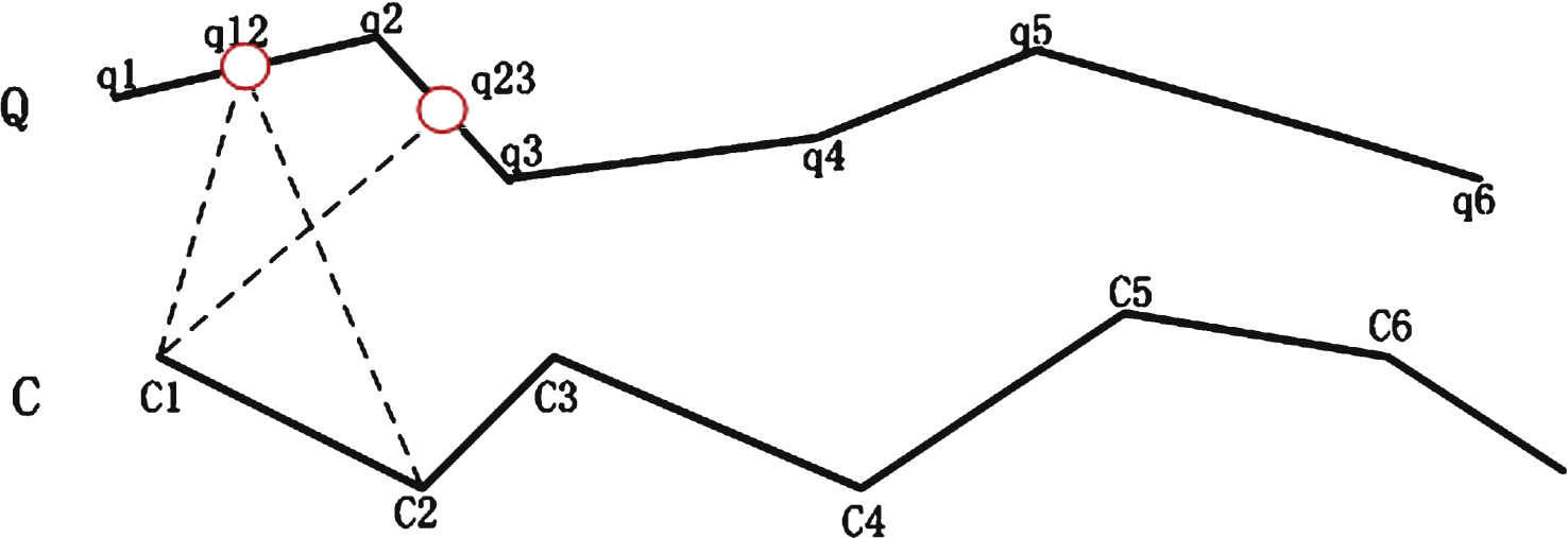
Fig.2
The clustering results produced by FTCBMOF and FCM (C = 4).
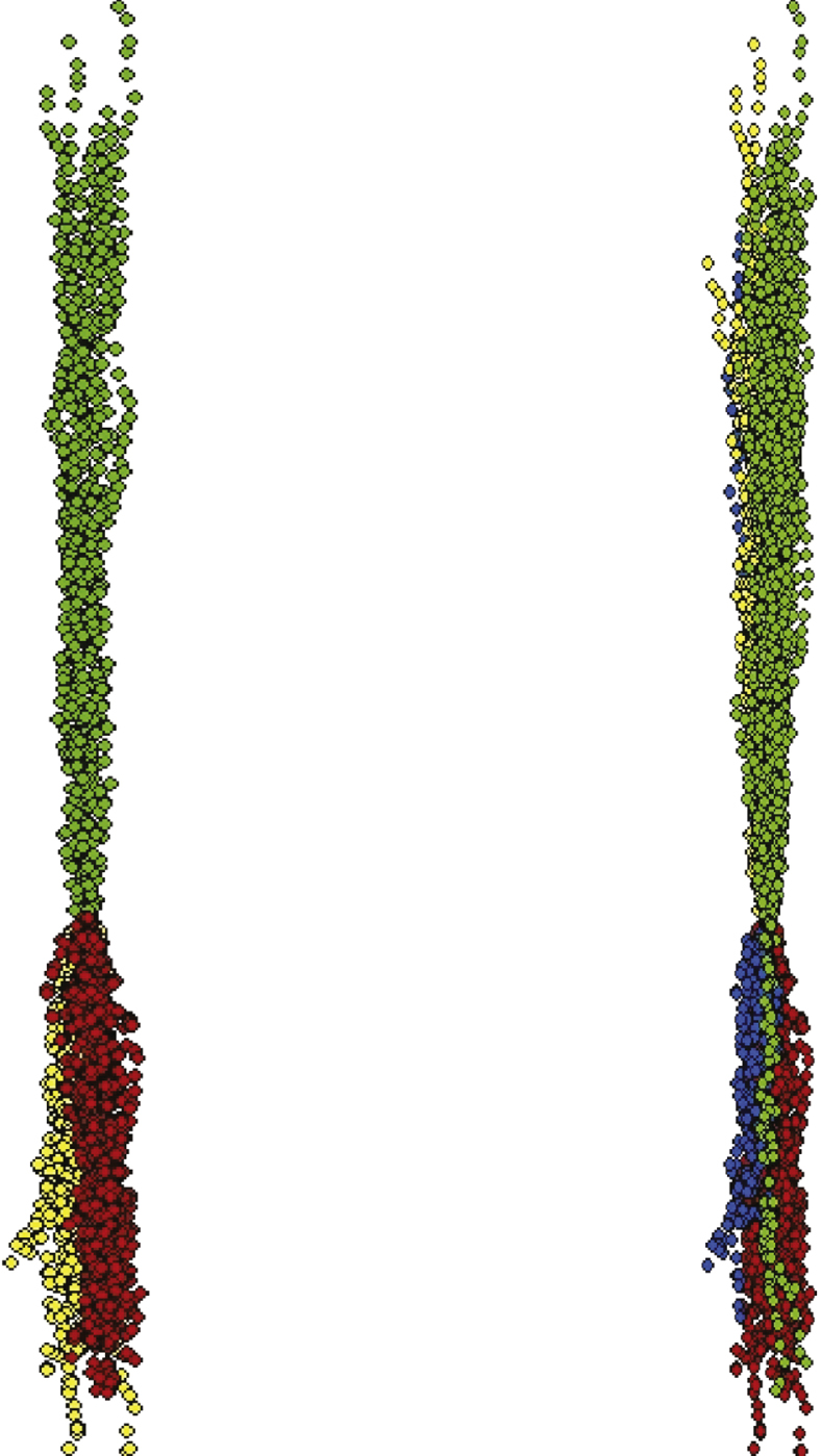
Fig.3
The clustering results produced by FTCBMOF (c = 6).
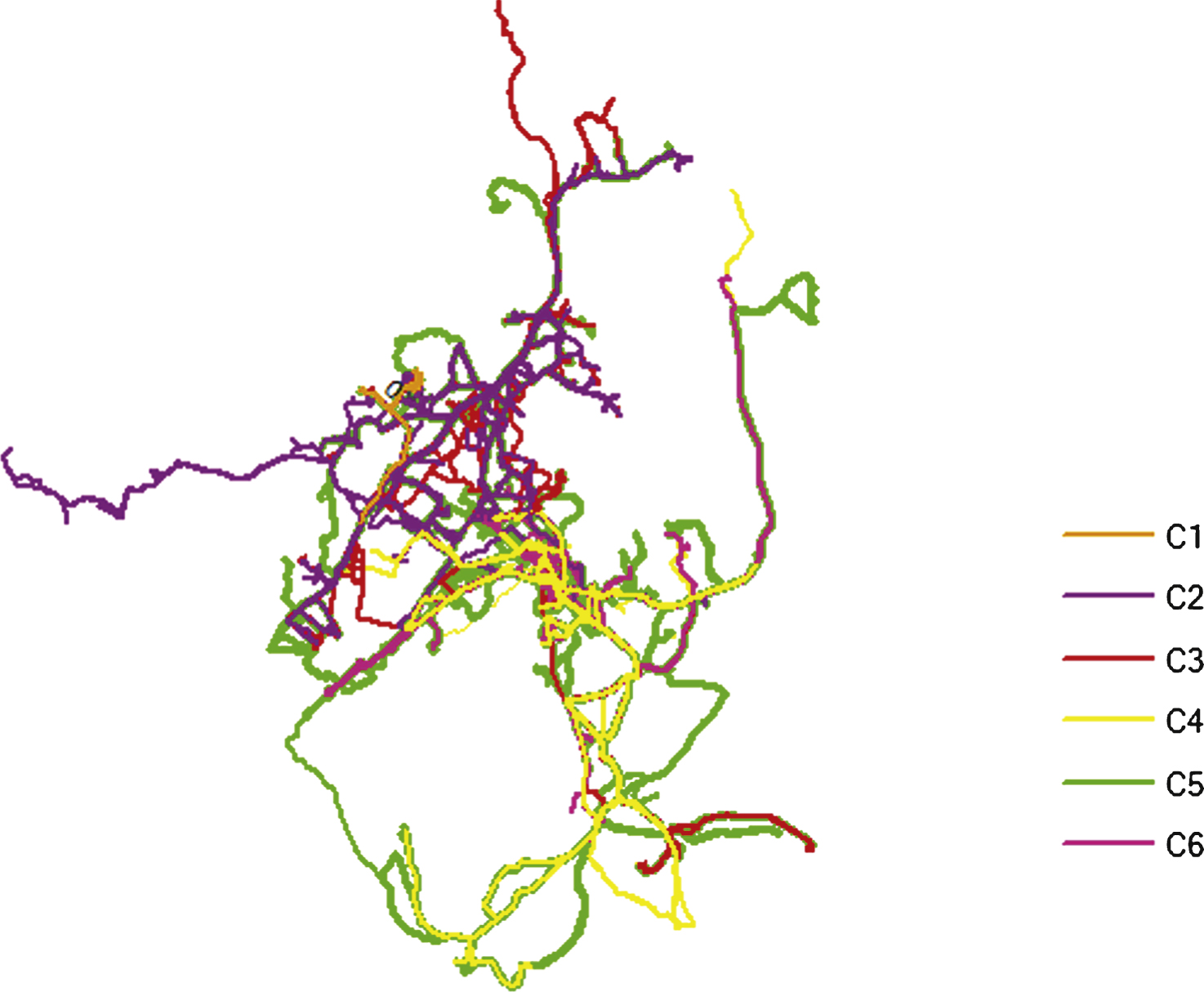
Fig.4
Hot spots from the cluster C1 to C6 produced by the new algorithm.
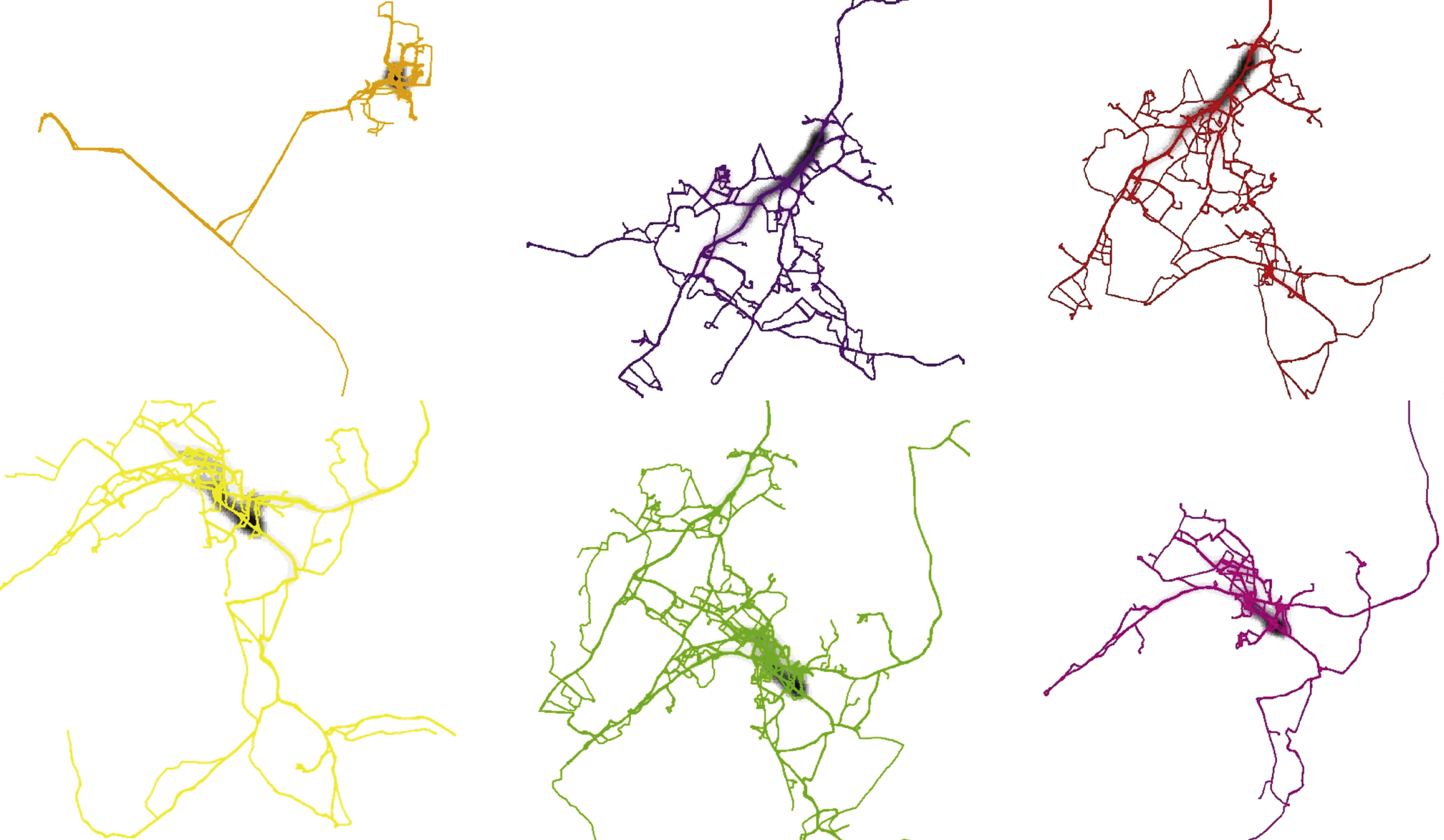
Fig.5
The hot spots in C1 cluster produced by FCM.
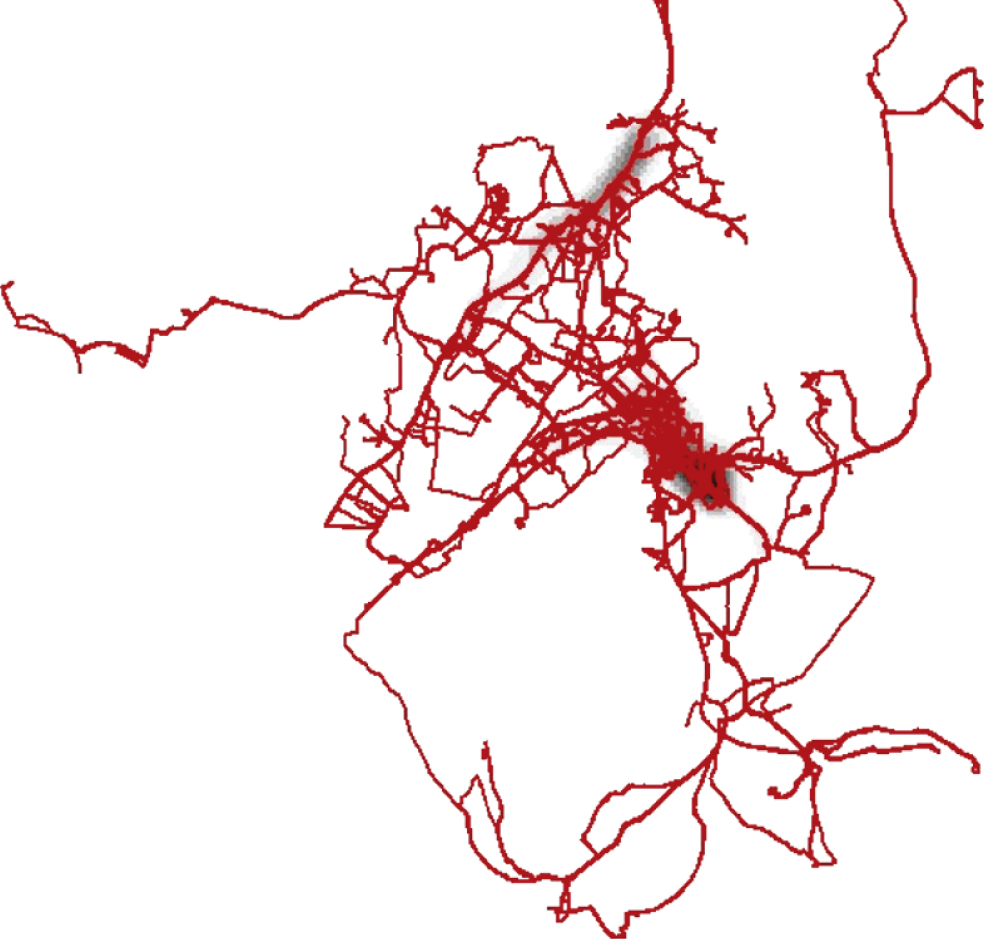
Fig.6
The hot spots in C2 cluster produced by FCM.
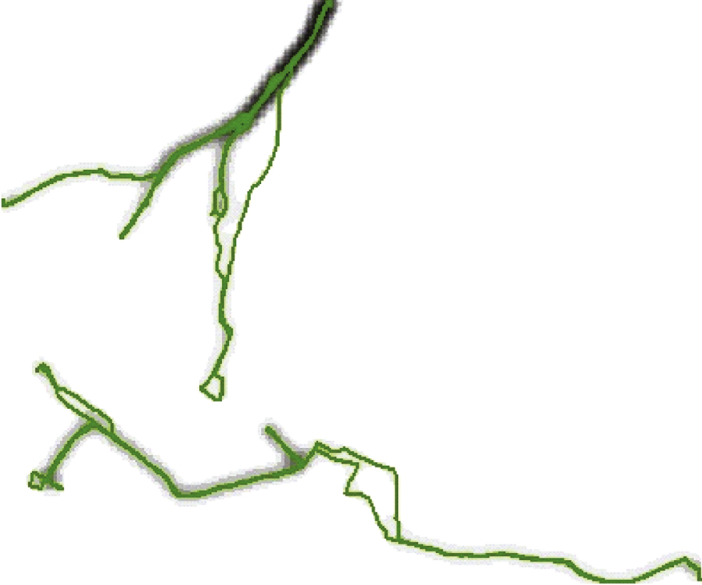
Table 1
Clustering validity evaluation result for synthetic data (c = 2)
| Validity indices | FTCBMOF | FCM |
| Jaccard | 1 | 0.49 |
| XB | 0.5 | 0.5 |
Table 2
XB index values for vehicle historical trajectory clustering
| c | FTCBMOF | FCM |
| 2 | 0. 937172 | 0.104377 |
| 3 | 0.7114215 | 0.416386 |
| 4 | 0.5401582 | 0.366364 |
| 5 | 0.4303577 | 0.253603 |
| 6 | 0.3586149 | 0.191558 |

