Fuzzy neural network-based robust adaptive control for dynamic positioning of underwater vehicles with input dead-zone
Abstract
This paper proposes a design for a robust adaptive controller for the Dynamical Positioning (DP) of underwater vehicles with unknown hydrodynamic coefficients, unknown disturbances and input dead-zones. First, for convenience of controller design, the Multi-Input Multi-Output (MIMO) system is divided into several Single-Input Single-Output (SISO) systems. Next, a Dynamic Recurrent Fuzzy Neural Network (DRFNN) with feedback loops is employed to approximate the unknown portion of the controller, which can greatly reduce the number of neural network inputs. A fuzzy logic dead-zone compensator is designed to cope with the unknown dead-zone characteristics of actuators. The upper bounds of the approximation errors and disturbances of the network, which are often used in existing works, are not necessary in this paper due to the presentation of a special robust compensator. Stability analysis is conducted according to the Lyapunov theorem, and the tracking error is proved to converge to zero. Simulation results indicate that the proposed controller demonstrates good performance.
1Introduction
Underwater vehicles have been widely used in marine missions for some time, for such uses as marine science, submarine rescue, data gathering, etc. For some specific tasks, the vehicles are required to precisely maintain positions near structure [3, 20]. Therefore, six Degree of Freedom (DOF) dynamic positioning controllers are necessary for these situations. Due to 6-DOF control issues, the design of controllers is complicated due to the existence of strong coupling character, nonlinear nature, unknown parameters and time-variable disturbances. Therefore, it is a significant and challenging task to design a 6-DOF controller with the ability to handle these factors.
Many researchers have made outstanding contributions to the control issues of underwater vehicles [22]. Mode-based controllers are often utilized in underwater vehicle systems, such as the Lyapunov method, backstepping technique, feedback linearization, and some combined methods [4, 18]. However, most controllers require an accurate mathematical model of the vehicle, which is often difficult to obtain. Adaptive controllers have been developed in many studies to overcome these problems by estimating the unknown and/or slowly-varying parameters [8, 21]. An adaptive PD controller for 4-DOF positioning of a Remotely Operated Vehicle (ROV) is discussed to maintain the position of the ROV close to an underwater structure [6], and the disturbing force caused by ocean current, passive arms, and umbilical cables are compensated for by adaptive estimation. Zhu and Gu proposed an MIMO nonlinear adaptive robust controller with estimated unknown hydrodynamic parameters and slowly varying disturbances [12].
Approximation-based control methods such as neural networks and fuzzy logic systems are also effective tools to overcome the limitations of the controller [24–26]. These methods are typically utilized to deal with the unknown terms, nonlinear terms or time-varying disturbances. Ishaque described an efficient fuzzy controller which reduced the conventional two-input fuzzy controller to a single-input fuzzy controller [13, 14]. The primary advantage of this approach was that rule inferences were greatly reduced and the calculation procedure was simplified. An adaptive fuzzy sliding mode controller with a novel fuzzy adaptation technique was presented for an Autonomous Underwater Vehicle (AUV) in the presence of external disturbances and parameter uncertainties. Li and Lee proposed an effective control method, in which the uncertain parameters of AUVs were approximated by a single hidden layered neural network [9]. Also they presented a semi-globally stable adaptive controller for diving control of an AUV, with a neural network to compensate for the unknown terms in pitch motion [10]. Wavelet Neural Networks (WNN) have great advantages in dynamic responses and information storing abilities [1, 2]. A WNN-based adaptive robust controller was investigated to resolve the MIMO tracking control system. Further study introduced a Recurrent Wavelet Neural Backstepping Control (RWNBC) scheme including a neural network and a smooth compensator, which was developed for MIMO systems. An adaptive output feedback controller for AUV was proposed by Zhang, and a Dynamic Recurrent Fuzzy Neural Network (DRFNN) was employed to estimate the dynamic uncertain nonlinear mapping [15]. Since there is an internal feedback loop in this type of neural network, the neural network is able to capture the dynamics of a system, requiring fewer network inputs than conventional neural networks. This paper employs a DRFNN approach to deal with the unknown portion in the ideal controller, which includes the uncertain parameters of the vehicles.
Robust controllers are well known for their immunity to disturbances, and have been widely used in underwater vehicles [5, 11, 16]. Robust terms were often employed to handle the approximation errors of neural networks, external disturbances, and estimation errors of adaptive controllers. However, the upper bounds of the signals were necessary to most existing works, which is difficult to implement in actualsystems.
Additionally, from a practical perspective, saturation and dead-zones of the actuators often exist, which will affect the performance of the DP system [19, 23]. This type of vehicle often uses thrusters as actuators, and thrusters have certain inherent nonlinear characteristics such as saturation and dead-zones. However, many control strategies ignored the saturation and dead-zones, due to their different control objectives. As to the DP system under investigation, the speed of the underwater vehicle of the system usually works at low or zero speeds. Also, the existence of the pre-filter will not cause large changes in the error vector, so that the controller outputs will barely reach saturation. Therefore, in this paper, only the effect of the dead-zone will be taken into account.
In current studies, the most common problems in the existing methods of underwater vehicles are as follows: a) AUV controllers are typically designed according to 3-DOF motion. Six-DOF control is more complicated and presents additional challenges; b) The derivation of the transform matrix is used in many controllers, which is very complex, and the derivation is difficult to obtain for the 6-DOF system; c) In some research, robust terms are used to suppress or offset the effect of jamming, and the upper limits of the disturbances are customarily necessary; d) Most controllers can ensure that the tracking error converges to a neighborhood of zero, which cannot satisfy the precision demands; e) The dead-zone of the actuator was not taken into account in many DP systems.
The primary contribution of this paper is to propose a DRFNN-based adaptive robust controller for 6-DOF underwater vehicles. The controller can be designed without explicit knowledge about the model of the vehicle, and the derivation of the transform matrix. A feed-forward fuzzy compensator is designed to eliminate the effects caused by dead-zones. Additionally, a special robust controller is developed to handle the approximation error of the neural network, estimation error and equivalent disturbances. The bounds of the disturbances are not necessary by utilizing the robust compensator, and the error can converge tozero.
The structure of this paper is organized as follows. Section II describes the control problem of underwater vehicles subject to uncertain terms and disturbances. Section III presents the design of the dynamic recurrent fuzzy neural network-based controller, a fuzzy dead-zone compensator and a robust controller. In section IV, simulation studies are described to verify the effectiveness of the proposed control scheme. Finally, conclusions are made in the finalsection.
2Problem formulation
2.1Underwater vehicles’ kinematics and dynamics
For the underwater vehicle positioning system, the kinematics and dynamics can be described by the following equations:
(1)
where
(2)
where J 1 ( η ) and J 2 ( η ) are complex functions of Euler angles φ, θ, ψ. By defining y = η = [y 1, …, y n ] T , system (1) can be rewritten as follows:
(3)
where
(4)
Choose τ i as the primary input value for the i-th sub-system. Then, the sub-system can be rewritten as follows:
(5)
where d si is the equivalent disturbance of the i-th sub-system. Therefore, the MIMO system is divided into six SISO systems. Assume that the equivalent disturbance of the i-th sub-system satisfies ∥d si ∥ ≤ D si , and g ii (x) ≥ g 0 > 0. D si and g 0 are unknown constants.
2.2Reference trajectory and control objective
Define the constant vector y d = [y d1, …, y dn ] T as the desired output value of the system. In order to make the differential of y d always meaningful and improve tracking performance, a smooth reference trajectory y ref = [y ref1, …, y refn ] T for the tracking system will be generated by the pre-filter:
(6)
where M r , D r , and G r are positive design matrices.
Remark: In order to ensure that the reference signals y
ref
,
The control objective is to devise a neural network-based adaptive output feedback controller τ, such that the output signal y follows a desired reference trajectory y ref , and the signals in the closed-loop system remain bounded.
3Adaptive robust controller design
In this section, an adaptive robust controller is employed for the DP system of an underwater vehicle.
Considering sub-system (5), the extensional error can be defined as follows:
(7)
where e i = y refi - y i is the tracking error of the i-th subsystem, and λ > 0 is a constant.
Therefore, the z i dynamics can be described as follows:
(8)
where
3.1Controller design without disturbances
An ideal controller is derived in this section for the z i dynamics under the assumption d si = 0:
(9)
Considering the Lyapunov function candidate asfollows:
(10)
Therefore, the derivative of function along the trajectory can be written as follows:
(11)
Thus, the asymptotic result is
Considering the ideal controller, the second term of the right side includes vehicle parameters. Let:
(12)
However, for 6-DOF underwater vehicles, it is often impractical to obtain all values in the system matrix, and the modelling error cannot be ignored. For these reasons, a DRFNN is employed to approximate the unknown function in controller, so the controller can be rewritten as:
(13)
3.2Dynamic recurrent fuzzy neural network
Different to traditional fuzzy neural networks, DRFNN with memory elements and an internal feedback loop can capture the dynamic response of a system. The derivatives
The DRFNN comprises five layers: input layer, fuzzy layer, fuzzy rule layer, normalized layer and output layer. The variables x N , y N are the input and output vectors of the neural network, respectively, and:
(14)
where
(15)
(16)
(17)
As shown by the above Equation (17), every rule application degree at time k not only contains the value at the current time, i.e.
The weight values
(18)
According to the approximation theorem [7, 17], there exist matrices W *, W R*, such that the continuous function on a compact set can be approximated by recurrent wavelet of the neural work, as follows:
(19)
where ∥ɛ ∥ < ɛ
N
, and ɛ
N
is the unknown upper bound of the reconstruction error ɛ. Since the optimal values are unknown,
(20)
where u si is the robust term to compensate for the approximate errors, and will be designed later.
3.3Adaptation laws
Define the estimation error vectors as follows:
(21)
Therefore, the reconstruction error of the RWNN can be written as follows:
(22)
where
(23)
Therefore, the reconstruction error
(24)
For the i-th sub-system, the adaptive laws are defined as follows:
(25)
where γ > 0, σ > 0 are the adaptive gain.
3.4Compensation of unknown dead-zone
However, when the speed of the vehicle is maintained around zero, especially with small disturbance forces, the engine of the thrusters must switch between forward and reverse in order to maintain the vehicle’s position. Direct application of the control law mentioned above will cause the motion of the vehicle to shock. Therefore, the effect introduced by the dead-zone of the thrusters should not be ignored. To compensate for the non-symmetric nonlinear dead-zone, a fuzzy logic (FL) feed-forward compensator is designed in this section.
The dead-zone nonlinearity of the actuator is shown in Fig. 2, and it can be written as follows:
(26)
where τ
i
is the controller output before the dead-zone abd T
i
is the output of the dead-zone, which represents the real control force acting on the vehicles; and
(27)
If (τ
i
∈ X
+ (τ
i
)) then
If (τ
i
∈ X
- (τ
i
)) then
where X + (·) and X - (·) are the membership functions (MFs) defined as follows:
(28)
Let d
i
= [d
i+, d
i-] T, X (τ
i
) = [X
+ (τ
i
) , X
- (τ
i
)]
T
. The forward compensator is designed here to compensate for the effect of the dead-zone, and make τ
i
≈ T
i
. The new control input
(29)
Therefore, when using a compensator, the real control force T i is expressed as follows:
(30)
where
(31)
As shown by the definition, ∥ϒ ∥ ≤ 1. UsingLyapunov’s direct method, the adaptive tuning law of the estimated dead-zone widths can be determined as follows:
(32)
3.5Final control scheme
To obtain the final controller, a robust term should first be designed to handle the errors.
Define the total residual error of the system as follows:
(33)
A special robust controller u si is chosen as follows to balance the estimation errors and the disturbances in the system, and make the tracking errors approach zero.
(34)
where
(35)
Remark: The existence of |z i | = z i sign (z i ) will result in chattering phenomenon when using the robust controller. In order to reduce chattering, the sign function sign (•) can be replaced by the hyperbolic tangent function tanh (•). This will not affect the stability of the system.
From the above sub-sections, the final control scheme is obtained, and which is illustrated in Fig. 3.
As shown in Fig. 3,
(36)
Therefore the final control law is comprised of a DRFNN controller
4Stability analysis
In this section, the stability of the designed control scheme will be proved. T i is the real control vector acting on the vehicle. Substituting Equation (30) obtains the z i dynamic, as follows:
(37)
Substituting the estimation error
(38)
By defining
(39)
Taking the time derivative of the Lyapunov function obtains the following:
(40)
Substituting the update laws of Equations (25), (32), and (35) into (40), obtains the following.
(41)
Since:
(42)
In the same way,
(43)
From the inequality of
(44)
Therefore,
(45)
Since the function
5Case study
To validate the proposed DRFNN-based robust adaptive controller, it is assessed in the MATLAB simulation environment with a 6-DOF nonlinear model of a vehicle. The desired position and attitude can be described as y d = [5 2 5 5 5 5] T .
Assume that the dead-zone widths are:
To verify the effectiveness of the controller and the control effect, unpredictable disturbances and parameter uncertainties are introduced. The environmental disturbances acting on the underwater vehicle and the uncertainties of the model can be treated together, as follows:
The pre-filter is utilized to produce a smooth target path for the controller, and the parameter matrices can be chosen as follows:
The reference trajectory generated by the pre-filter is shown in Fig. 4.
As shown by the control law in Equation (37), results indicate that the feedback gain K i is similar to the proportional of the PID controller. According to experience and multiple simulation results, an appropriate value of K i can be obtained. The controller parameters were chosen as:
A DRFNN with ten nodes in the product layer is used in the control system; the input vector of the neural network is
The parameters of the robust controller are chosen as γ
Δ
= 0.1. The initial value of
The 3-D trajectory of the vehicle is shown in Fig. 5, indicating that the proposed controller can drive the vehicle from the initial position y 0 = [0 0 0 0 0 0] T to the given position y d .
Figure 6 shows the curves of the vehicle’s position and attitude; the red lines represent the outputs of the pre-filter, and blue lines are the time history of x, y, z, φ, θ, ψ. As shown by the curves, the output of the vehicle can follow the reference trajectory well. The blue line represents a case with dead-zone compensation, while the red line represents a case without dead-zone compensation.
Figure 7 shows the time history of the error function with and without dead-zone compensation. As shown by Fig. 7, the error function reaches zero at 15–25s using the proposed controller. The performance of the controller is also improved by using dead-zonecompensation.
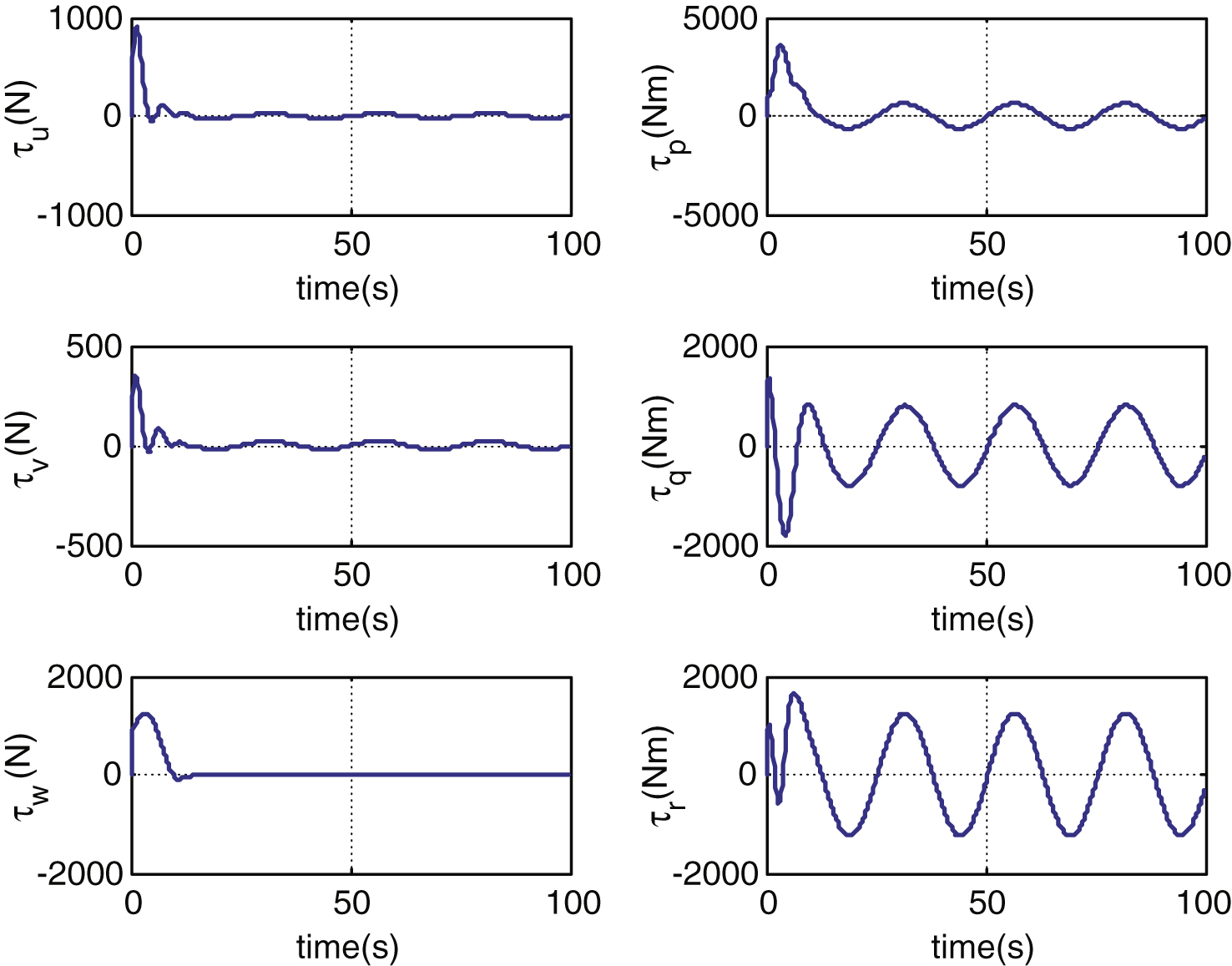
Figure 8 shows the curves of control inputs by using the proposed method. In general, the better tracking precision requires greater efforts, and may cause oscillations in control. As shown in Fig. 5, there are few slight oscillations at the beginning due to the existence of the DRFNN, but the outputs of the thruster are smooth and steady. In addition, the given signals required by the controller are given by the pre-filter, so the errors change smoothly and slowly, ensuring that the magnitude of the thruster can never achieve maximum values.
6Conclusions
This paper investigated the problem of location maintenance for underwater vehicles with parameter uncertainties and unknown external disturbances. At first, the MIMO system was divided into several SISO systems via transformation so that the output of the system was decoupled from the control input. Next, A DRFNN approach is used to estimate the unknown term in the ideal controller, and a special robust controller is designed to compensate for the approximate and equivalent errors. The effect of the dead-zone is eliminated by a fuzzy logic system. The tracking errors can converge to zero. The excellent performance of the aforementioned control scheme is validated by simulation for location maintenance of an underwater vehicle.
7Conflict of interests
The authors declare that there are no conflicts of interest regarding the publication of this article.
References
1 | Chen CH, Hsu CF (2010) Recurrent wavelet neural backstepping controller design with a smooth compensator Neural Computing and Applications 19: 7 1089 1100 |
2 | Chen CH (2012) Wavelet-based adaptive robust control for a class of MIMO uncertain nonlinear systems Neural Computing and Applications 21: 4 747 762 |
3 | Conrado de Souza E, Maruyama N (2007) Intelligent UUVs: Some issues on ROV dynamic positioning IEEE Transactions on Aerospace and Electronic Systems 43: 1 214 226 |
4 | Zhang G, Yu L, Meng X, Zhang L (2011) Tracking control of under actuated ship based on partial state feedback scheme Proceedings of 2011 IEEE/ICME International Conference on Complex Medical Engineering 678 683 Harbin |
5 | Yang H, Zhang F (2012) Robust control of formation dynamics for autonomous underwater vehicles in horizontal plane Journal of Dynamic Systems, Measurement, and Control 134: 3 031009 |
6 | Nguyen Quang H, Kreuzer E (2007) Adaptive PD-controller for positioning of a remotely operated vehicle close to an underwater structure: Theory and experiments Control Engineering Practice 15: 4 411 419 |
7 | Naira H, Flavio N, Nakwan K (2002) Adaptive output feedback control of uncertain nonlinear systems using single-hidden-layer neural networks IEEE Transactions on Neural Networks 13: 1420 1431 |
8 | Li JH, Lee PM (2005) Design of an adaptive nonlinear controller for depth control of an autonomous underwater vehicle Ocean Engineering 32: 18 2165 2181 |
9 | Li JH, Lee PM (2002) Neural net based nonlinear adaptive control for autonomous underwater vehicles IEEE International Conference on Robotics and Automation 2: 1075 1080 |
10 | Li JH, Lee PM (2005) A neural network adaptive controller design for free-pitch-angle diving behavior of an autonomous underwater vehicle Robotics and Autonomous Systems 52: 2 132 147 |
11 | Petrich J, Stilwell DJ (2011) Robust control for an autonomous underwater vehicle that suppresses pitch and yaw coupling Ocean Engineering 38: 1 197 204 |
12 | Zhu KW, Gu LY (2011) A MIMO nonlinear robust controller for work-class ROVs positioning and trajectory tracking control 2011 Chinese Control and Decision Conference 2565 2570 Mianyang |
13 | Ishaque K, Abdullah SS, Ayob SM (2010) Single input fuzzy logic controller for unmanned underwater vehicle Journal of Intelligent and Robotic Systems 59: 1 87 100 |
14 | Ishaque K, Abdullah SS, Ayob SM (2011) A simplified approach to design fuzzy logic controller for an underwater vehicle Ocean Engineering 38: 1 271 284 |
15 | Zhang LJ, Qi X, Pang YJ (2009) Adaptive output feedback control based on DRFNN for AUV Ocean Engineering 36: 9 716 722 |
16 | Lapierre L, Jouvencel B (2008) Robust nonlinear path-following control of an AUV IEEE Journal of Oceanic Engineering 33: 2 89 102 |
17 | Hovakimyan N, Nardi F, Calise A (2002) A novel observer based adaptive output feedback approach for control of uncertain systems IEEE Transactions on Automatic Control 147: 1310 1314 |
18 | Nambisan PR, Singh SN (2009) Multi-variable adaptive back-stepping control of submersibles using SDU decomposition Ocean Engineering 36: 2 158 167 |
19 | Selmic RR, Lewis FL (2000) Deadzone compensation in motion control systems using neural networks IEEE Trans Automat Contrl 45: 4 602 613 |
20 | Savaresi SM, Previdi F, Alessandro D, Sergio B (2004) Modeling, identification, and analysis of limit-cycling pitch and heave dynamics in ROV IEEE Journal of Oceanic Engineering 29: 407 417 |
21 | Wu TZ, Juang YT (2008) Adaptive fuzzy sliding-mode controller of uncertain nonlinear systems ISA Transactions 47: 3 279 285 |
22 | Fossen TI (2011) Handbook of Marine Craft Hydrodynamics and Motion Control John Wiley & Sons Chichester, West Sussex, UK |
23 | Zhang TP, Ge SS (2008) Adaptive dynamic surface control of nonlinear systems with unknown dead zone in pure feedback form Automatica 44: 1895 1903 |
24 | Pan Y, Yu H, Er MJ (2014) Adaptive neural PD control with semiglobal asymptotic stabilization guarantee IEEE Trans on Neural Networks and Learning Systems 25: 2264 2274 |
25 | Pan Y, Meng JE, Huang D, Wang Q (2011) Adaptive fuzzy control with guaranteed convergence of optimal approximation error IEEE Transactions on Fuzzy Systems 19: 5 807 818 |
26 | Pan Y, Meng JE (2013) Enhanced adaptive fuzzy control with optimal approximation error convergence IEEE Transactions on Fuzzy Systems 21: 6 1123 1132 |
Figures and Tables
Fig.1
The structure of DRFNN.
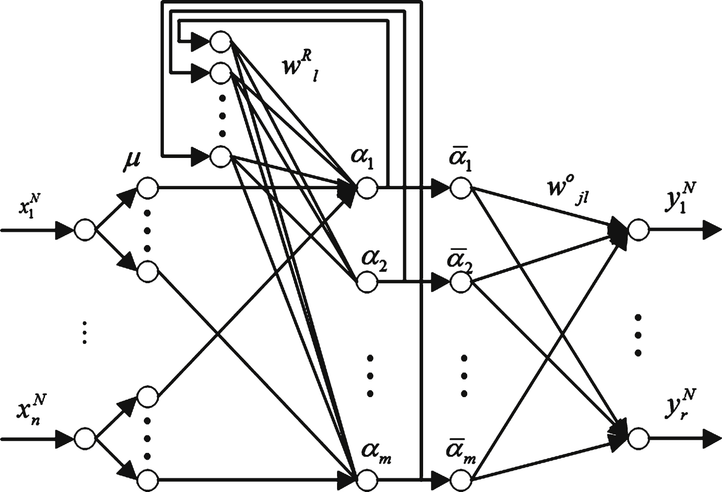
Fig.2
Dead-zone nonlinearity.
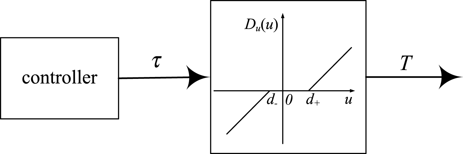
Fig.3
Architecture of the underwater vehicle control system.
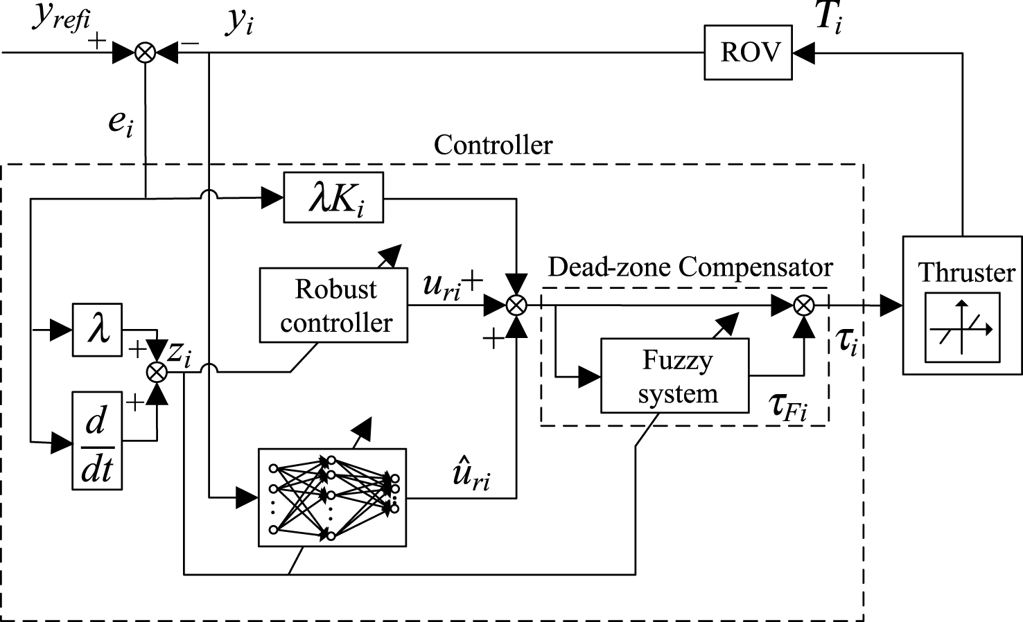
Fig.4
The reference trajectory generated by the pre-filter.
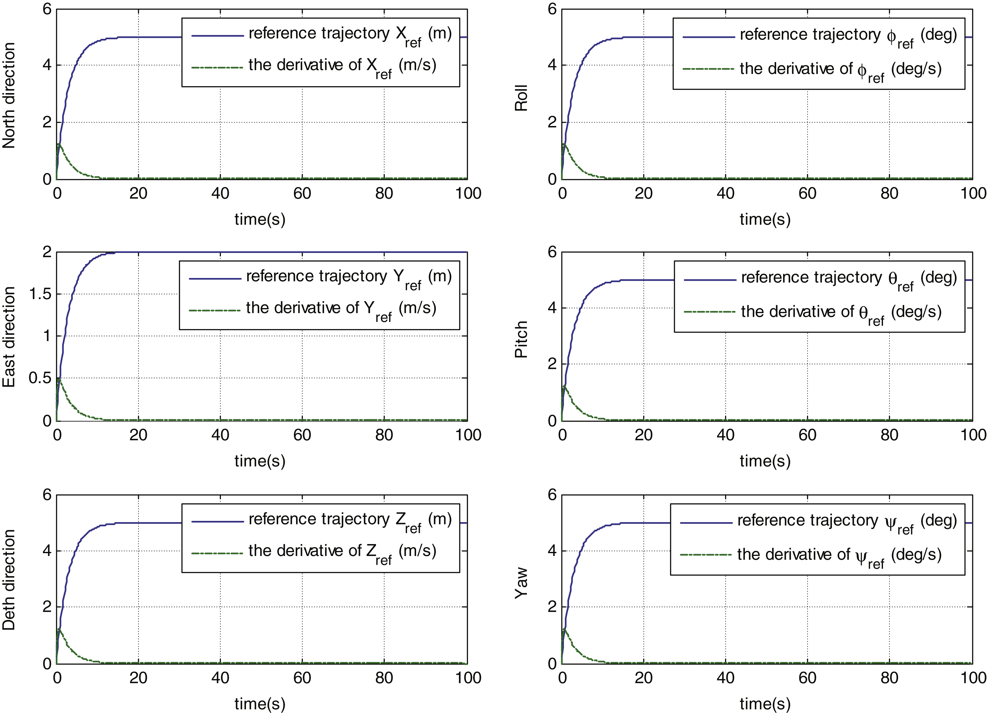
Fig.5
3-D trajectory of the underwater vehicle.
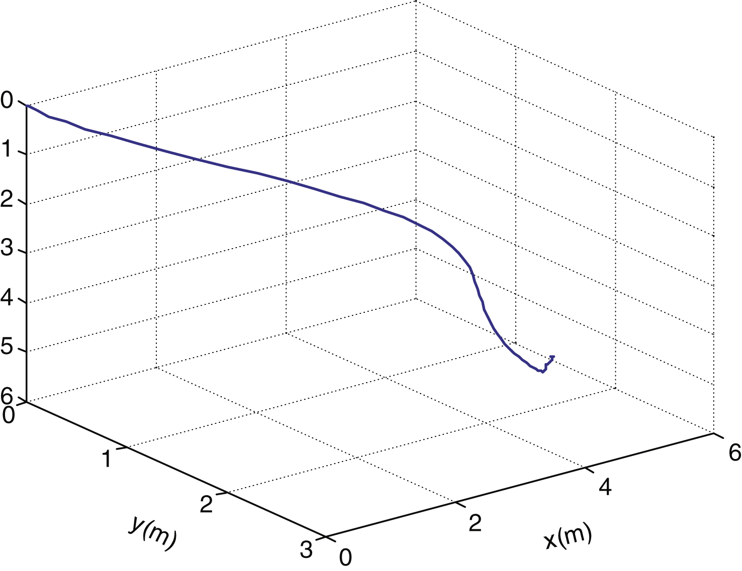
Fig.6
The trajectory of the underwater vehicle.
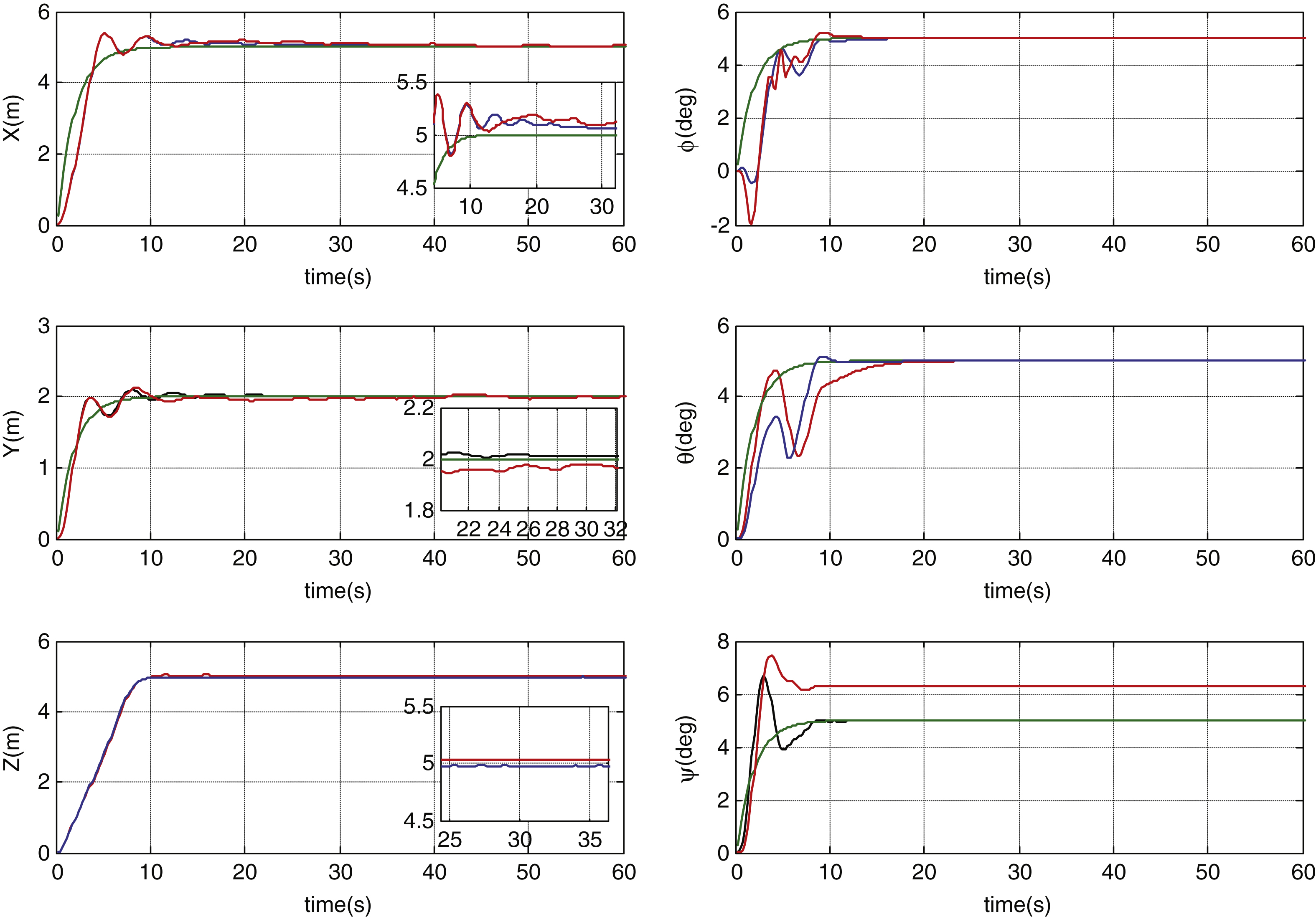
Fig.7
The time history of the extensional error function.
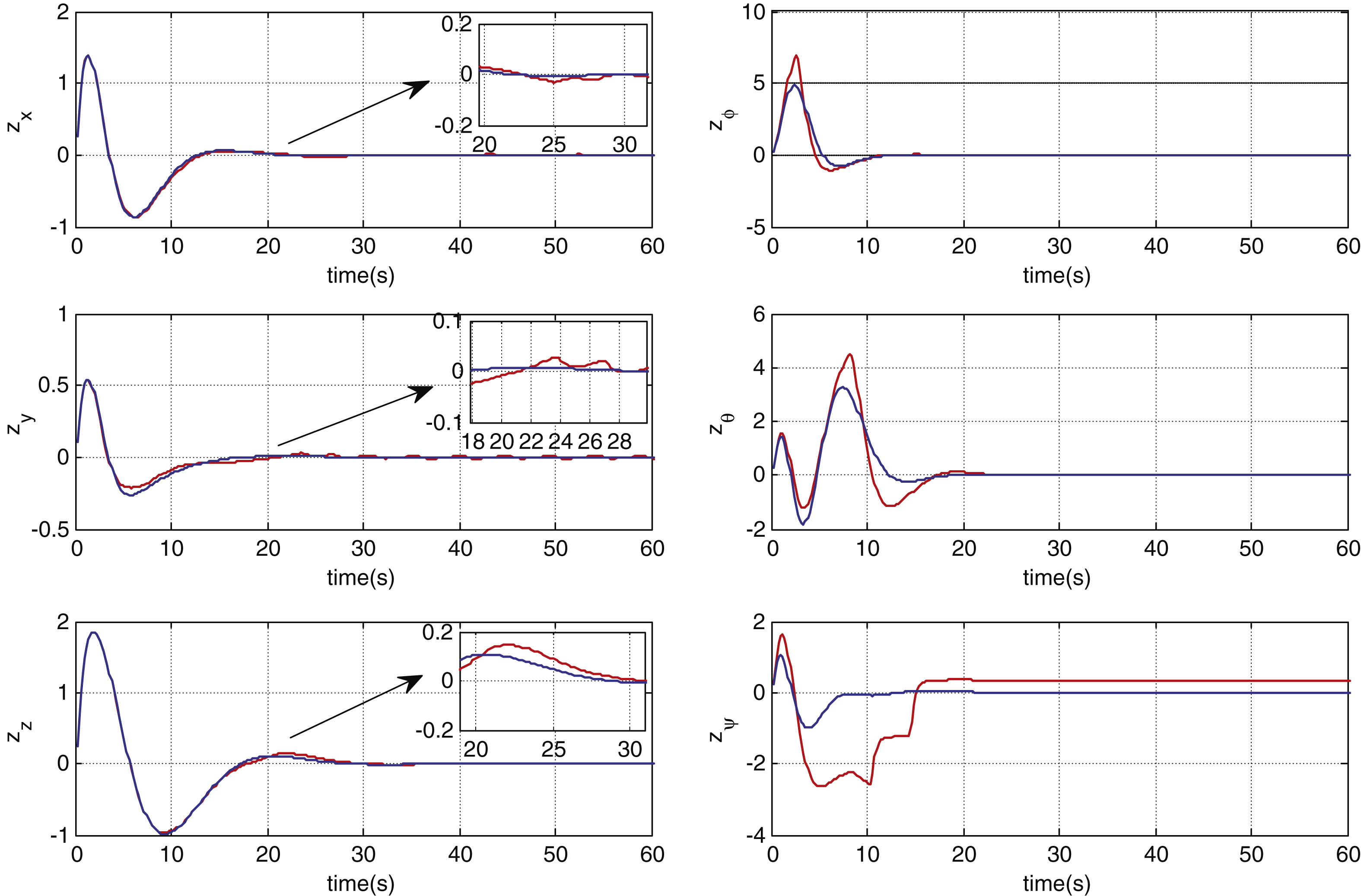
Fig.8
Control input using the proposed controller.