
Fuzzy PID control method of deburring industrial robots
Abstract
This paper proposes a fuzzy PID control method for deburring industrial robots. The adaptive fuzzy PID controller relates to the trajectory and joint angular parameters of the end-effector on a robot. The PID controller parameters update online at each sampling time to guarantee trajectory accuracy of the end-effector. The simulation of the fuzzy PID control is provided based on the 6-DOF deburring industrial robot. Experimental results demonstrate the efficiency of the fuzzy PID control method.
1Introduction
Industrial robots are used in industrial applications such as welding, grinding, and painting. It is therefore important that end-effector of such robots moves accurately and smoothly to achieve the desired trajectory.
This paper studies the aluminum casting of motorcycle accessories. Aluminum burrs are of irregular shapes and large volumes. Workers typically remove burrs, but this process can lead to injuries if the artificial manufacturing method is out of date.
This paper proposes an industrial deburring robot, which is safer and more efficient than the manual removal of burrs. The burr removal process is complicated because each burr is unique, and therefore requires special steps. Some experts suggest the use of the force/position control strategy to guarantee product accuracy [6]. This paper introduces an effective online force control direction adjustment algorithm using the fuzzy vector method.
The workpiece and tool should be taken into account during manufacturing. An adaptive fuzzy hybrid position/force controller was proposed [4]. The removed material should also be taken into account. An adaptive modeling method based on statistic machine learning was proposed [18], as was an intelligent control method for the industrial robot was proposed [19]. A nonlinear damping control scheme that reduces the force overshoot without compromising the dynamic response was proposed [2]. A solution of unmanned helicopters using a novel nonlinear model predictive controller enhanced by a recurrent neural network has also been proposed [7].
A new methodology based on a multi-objective genetic algorithm was proposed [12]. An algorithm designed for high-accuracy local dynamic identification was presented [10]. A novel method to study precision grip control using a grounded robotic gripper with two moving, mechanically-coupled finger pads equipped with force sensors was presented [11]. A fuzzy reinforcement learning (FRL) scheme based on fuzzy logic and the sliding-mode control was presented [13].
The position and orientation of the end-effector are important for the deburring robot. The end-effector orientation and position freedom, as well as the robot configuration, greatly influences the cost of supporting movement [14]. The design and implementation of a platform for rapid external sensor integration into an industrial robot control system was presented [1].
The intelligent control methodology is used to solve sophisticated tasks. The intelligent controller work condition, which takes into account human expert knowledge and skills for planning and controlling sophisticated tasks, was introduced [8, 16].
A method of path planning was introduced for automatic grinding robotic blade. The robot program, which contains the grinding path generated by a PC, was demonstrated [20]. A controller based on a GA-fuzzy-immune PID, a robot dexterous hand control system, and a mathematical model of an index finger were also presented [17]. Co-simulations of a novel exoskeleton-human robot system based on humanoid gaits with Fuzzy PID algorithms was presented [3].
Vibration suppression in a two-inertia system using an integration of a fractional-order disturbance observer and a single neuron-based PI fuzzy controller was presented [15]. A collocated proportional-derivative (PD)-type Fuzzy Logic Controller (FLC) was developed, which was used to study controller effectiveness [9]. The hierarchical fuzzy logic is provided according to the singular perturbation approach, which can derive the slow and fast subsystem of a flexible-link robot arm control [5].
Traditional PID parameters could not be modified. However, the advantages of the PID control method are the easy measurement of parameters, which is helpful in choosing optimal values.
The fuzzy rules of the fuzzy control strategy are difficult to determine. The parameters of the Fuzzy PID strategy can be updated online according to the practical conditions. In this paper, PID parameters are modified according to actual working conditions. Robot control efficiency and accuracy is improved based on the fuzzy PID algorithm. The paper is organized as follows: Section 2 introduces the robotic system and manipulator kinematics; Section 3 presents the traditional PID controller and mathematical model; Section 4 details the fuzzy control approach; Section 5 describes the fuzzy PID controller design and improvements; Section 6 compares the simulations between the traditional and fuzzy PID controller; and Section 7 summarizes theconclusions.
2The introduction and model of the robot system
Figure 1 shows the 6-DOF deburring industrial robot. It is composed of a base, waist, arm, and manipulator. The robot kinematic model is described by homogeneous coordinates.
2.1Manipulator kinematics
Manipulator kinematics involve geometric and time-based motion properties, particularly the interactions between the various links over time. In this paper, the manipulator kinematics are described by the D-H method. The six links are built in separate coordinates; their positions and orientations are described in the coordinates. Table 1 describes the four parameters a i-1, α i-1, d i , θ i .
2.2Kinematics model based on D-H notation and ER50-C20 link parameters
There are some relative parameters on the ER50-C20:
a 1= 220 mm, a 2= 900 mm, a 3= 160 mm, d 1=563 mm, and d 4= 1014 mm.
According to the inverse kinematics solution method, the angular joint of the end-effector can be calculated as follows:
(1)
The manipulator kinematics were discussed and the kinematic model based on D-H notation was built. The relationship between the position p = (p x , p y , p z ) of the end-effector and the angular joint θ is obtained. According to the known end of the link relative to the position and orientation of the reference coordinate system, the inverse kinematics are used to calculate each joint variable. The error between the desired angular joint and actual angular joint is regarded as input. The following sections describe the PID mathematical model.
3The PID controller model in a deburring robot
In an ER50-C20 robot, the machining path of the following workpieces is machined according to the machining path predetermined by the related numerical value of the terminal trajectory, recorded by a coded disk and the artificial teaching method. The optimal machining path can be achieved by proper adjustments to meet the accuracy requirements. If the desired trajectory is known, the PID controller is placed into the above linear system.
(2)
(3)
Therefore, the transfer function is obtained asfollows:
(4)
As shown in Fig. 2, a desired trajectory is obtained by the teaching method, and the desired position of the end-effector X d is obtained. The desired joint angular θ d of the end-effector is calculated by inverse kinematics, as described by Equation (1). The desired joint angular θ d is output by the PID controller and the robot model. This represents the teaching method process. When the second workpiece is deburred, the value e = (θ d - θ) is regarded as the input. The error e is the output of the PID controller and robot model. The optimal actual joint angular θ is calculated, and the actual joint angular θ is recorded by a coded disk. The next workpiece is manufactured in this way.
Though the traditional PID controller could detect the parameter values of the end-effector, the shortage of the traditional PID algorithm is evident because its parameters cannot self-adjust to control complex, nonlinear subjects; thus, this method may create errors when the current workpiece is different from the previous one. Fuzzy PID can be applied to this robot, enabling it to cope with the difficulty of complicated nonlinear systems. A fuzzy PID algorithm can self-adjust parameters according to rules designed by experience.
4The fuzzy PID control approach
The fuzzy controller can measure the outputs of the traditional PID controller and alter them in order to reduce output errors. The fuzzy controller can make accurate decisions to improve machining accuracy based on the knowledge of human operation and experience. The fuzzy controller has integral fuzzy sets, which are designed by work conditions; these fuzzy sets are small, medium, large, etc. The fuzzy sets can be converted into the automatic control strategy based on a knowledge base. The fuzzy controller consists of fuzzification, fuzzy reasoning, defuzzification, and the knowledge base. When the fuzzy sets have been designed, the inputs must adapt to the corresponding rules. The output values can be obtained by fuzzy reasoning based on fuzzy rules; better output values acquire better results. Finally, inputs have m fuzzy values; the number of rules are represented by m n , where n is the number of inputs.
5The fuzzy PID control algorithm
5.1The design of the fuzzy PID controller
The fuzzy PID controller meets e and ec requirements for PID parameters at different times. Figure 3 depicts the basic process.
The fuzzy PID control system is composed of the input, output, and feedback loop. The error and error rate of the joint angular of the end-effector are regarded as the inputs, and the three parameters K
p
, K
i
, K
d
represent the outputs. As shown in Fig. 7, the controller consists of the traditional PID controller and fuzzy controller. The three parameters K
p
, K
i
, K
d
of the traditional PID controller are updated online by the fuzzy rules. The fuzzy rules are designed in the fuzzy controller. The values e = θ
d
- θ and
The proper actual joint angular θ is obtained. In each control loop, the error and error rates between the input signals and feedback signals are controlled by the fuzzy PID controller. Figure 8 shows a detailed fuzzy PID controller structure; the fuzzy rules are shown as Equations (5). The fuzzy subset is {NL, NM, NS, ZE, PS, PM, PL} and the fuzzy domain is {–0.3, –0.2, –0.1, 0, 0.1, 0.2, 0.3}, in which the NL, NM, NS, ZE, PS, PM, and PL stand for negative large, negative middle, negative small, zero, positive small, positive middle and positive large, respectively. The value of e represents the error and ec represents the error rate. The triangle-type membership function is adopted for each fuzzy variable, as shown in Figs. 4–6, which show the membership function curves of e, ec, dK p , dK i , dK d , respectively.
The number of fuzzy sets is chosen based on the desired manufacturing needs and workpiece quality. In general, there is no specific method for designing the fuzzy controller, but input and output membership functions to emulate human decision-making can be designed. The following methods are typically used to design a fuzzy controller:
– Model the knowledge of the control engineer.
– Model of the actions and experience of the human operator.
– Fuzzy model of the controlled plant.
As shown in Fig. 8, the error between the desired joint angular θ d and the actual joint angular θ of the end-effector is regarded as the input, noted by e. The value of e is fuzzy according to the fuzzy controller, used in fuzzy operators. The process is fuzzy reasoning, which obtains the optimal fuzzy value. The optimal fuzzy value should be defuzzified to obtain the clear value, which is used in the mathematical model of the robot.
5.2Design of control rules of K p , K i , K d
Three positive trapezoidal fuzzy sets are required to cover the input and output variables.
The material of the workpiece is aluminum and the material of the tool is cast iron. The analysis of force between the tool and the workpiece should be considered. Combining the experience of the workers and work conditions, three different fuzzy rules for each gain are utilized, and the three parameters K p , K i , K d can be designed based on the analysis. Test results indicate that K p = 4, K i = 0.001, K d = 100 could be properly applied to the traditional PID controller and the fuzzy PID controller. The fuzzy rules should be clearly classified in order to increase effectiveness. However, too many rules will have a negative impact on system stability. According to the work condition, if the fuzzy sets have less than two rules, the fuzzy subset will become {NL, NS, ZE, PS, PL}. Because the workpiece is shaped irregularly, two rules are not able to meet the change requirement, which should be variable based on the blur amount. However, if there are too many rules, the end-effector stability will decrease. Therefore, three fuzzy sets are more reasonable. The fuzzy subset is {NL, NM, NS, ZE, PS, PM, PL}.
5.2.1Design of control rules of K p
In the PID system, the response speed and steady-state error are affected by the value of K p . At the beginning of the regulation, the value of K p is increased to obtain faster response speeds. In the middle of the regulation, the smaller overshoot and faster response speed must be considered, and the value of K p decreases. Increasing K p at the end of the regulation promotes machining precision. ΔK p is the compensation amount. The fuzzy domain of ΔK p is {–0.03, –0.02, –0.01, 0, 0.01, 0.02, 0.03}, which corresponds to {NL, NM, NS, ZE, PS, PM, PL}.
5.2.2Design of control rules of K i
In the PID system, the integral control eliminates the steady-state error of the system. At the beginning of the regulation, K i is reduced to prevent integral saturation. In the middle of the regulation, K i is increased to guarantee system stability. At the end of the regulation, the static error is reduced by increasing K i . ΔK i is the compensation amount. The fuzzy domain of ΔK i is {–0.03, –0.02, –0.01, 0, 0.01, 0.02, 0.03}, which corresponds to {NL, NM, NS, ZE, PS, PM, PL}.
5.2.3Design of control rules of K d
In the PID system, the differential control can change the dynamic characteristics. At the beginning of the regulation, K d is increased to prevent overshooting. In the middle of the regulation, K d is reduced to a constant. At the end of the regulation, K d is further decreased to reduce the settling time. ΔK d is the compensation amount. The fuzzy domain of ΔK d is {–0.3, –0.2, –0.1, 0, 0.1, 0.2, 0.3}, which corresponds to {NL, NM, NS, ZE, PS, PM, PL}.
5.3The rules of fuzzy control
(1) When |e| is a greater value, ΔK p must also be bigger, ΔK d should be smaller, and ΔK i = 0.
(2) When |e| is a middle value, ΔK p should decrease, and ΔK d and ΔK i should be of middle value.
(3) When |e| is a smaller value, ΔK p and ΔK i should be greater, and ΔK d should be a middle value.
The rules of the Fuzzy PID controller are as follows:
(5)
There are 49 rules in the fuzzy logical controller, as shown in Tables 2–Tables 4. In this paper, 49 fuzzy rules were considered necessary and created to implement the proposed fuzzy PID controller for the deburring robot system. The PID parameters were updated online according to these rules. The inputs of the fuzzy logic block are the angular displacement error e and derivative of error ec. The inputs are modified by the fuzzy PID feedback system to optimize the trajectory. According to the fuzzy rule tables, the PID parameters are modified as follows:
(6)
The output of the fuzzy PID algorithm are as follows:
(7)
5.4Output defuzzification
The center average method was used for defuzzification. The output u is calculated as:
(8)
If the input is known, the output can be calculated by Equations (8). Combining Equations (7) and (8), K p , K i , K d are obtained to control the end-effector trajectory. K p , K i , K d are adjusted by the fuzzy PID under actual processing conditions. The simulations in the next session verify the feasibility of the traditional PID and the fuzzy PID algorithm.
6Experiments and simulation analysis
The methods described in this paper have been tested in simulations of the ER50-C20 robot. Given the original value of joint θ= [0.176, –0.701, 0.079, –0.0002, –0.949, –1.019] and the final value of joint θ′= [–0.236 –0.166 –0.691 0 –0.715 –0.237]. The end-effector of the robot moves from point A (1350, 530, 1250) to point B (1615, 240, 490) in Cartesian space. A total of 101 points were sampled between A and B. The sample time was 5 seconds, sampled once every 0.05 seconds.
Figure 9 shows the trajectory curves simulated by the Matlab toolbox; the curves are formed by interpolation. The end-effector trajectory is determined by the artificial teaching method, as shown in Fig. 9, which also indicates the three dimensional trajectory of the end-effector.
The traditional PID method requires a long setting time of approximately 1s, as shown in Fig. 10. The error curve is shown in Fig. 11. The red solid line represents the fuzzy PID control method; the black dotted line represents the traditional PID control method. The fuzzy PID algorithm requires a short setting time of 0.3s, as shown in Fig. 10. Figure 11 depicts the corresponding error curve. The fuzzy PID control strategy error value is approximately 10–4 rad in Fig. 11. The error value of the traditional PID control method is approximately 0.01rad, as shown in Fig. 11. This indicates that the fuzzy PID controller is more accurate than the traditional PID controller. Comparing the red solid line to the black dotted line in Fig. 10, the setting time of the black dotted line is more than 3 times that of the red solid line. Thus, the fuzzy PID controller has a shorter setting time than the traditional PID controller. The fuzzy PID overshot by approximately 7.5% , which is within the permitted 20% scope. The overshot value has small impact on the workpiece, and results meet the requirements.
According to the simulation, the setting time is greatly reduced and the joint angular error is decreased for the fuzzy PID controller. The fuzzy PID controller performs better than the traditional PID algorithm. As shown in Fig. 12, K p is updated online by the fuzzy PID algorithm, and the optimal value of K p is obtained according to the actual processing conditions. As shown in Figs. 13 and 14, the values of K i and K d are updated online. The fuzzy PID controller values of K p , K i , K d are more accurate than the parameters of the traditional PID.
7Conclusion
This paper presents a fuzzy PID control algorithm. The controller parameters are updated online at each sampling time; traditional PID parameters cannot update online. The fuzzy PID algorithm improves efficiency and accuracy. This proposed control strategy is easy to implement. The simulation results indicate that the fuzzy PID algorithm meets the demands of deburring processing. Compared to the traditional PID controller, the fuzzy PID controller guarantees the stability of the closed-loop system and chooses the proper parameters according to the control rules. The uncertainties are detected online, therefore allowing adaptive compensation for error.
Acknowledgments
This work was supported by the Youth Science Fund Project NO.61305116 of the National NaturalScience Foundation, and Major Science and Technology Projects of Chongqing Robot Industry No.cstc2013jcsf-zdzxqqX0005.
References
1 | Robertsson A, Olsson T, Johansson R, BlomdellK Nilsson A, Haage M (2006) Implementation of industrial robot force control case study: High power stub grinding and deburring IEEE International Conference on Intelligent Robots and Systems 2743 2748 |
2 | Lai CY (2014) Improving the transient performance in robotics force control using nonlinear damping IEEE International Conference on Advanced Intelligent Mechatronics 892 897 |
3 | Pan D, Gao F, Miao YJ, Cao R (2015) Co-simulation research of a novel exoskeleton-human robot system on humanoid gaits with Fuzzy PID/PID algorithms Advances in Engineering Software 79: 36 46 |
4 | Hsu FY, Fu LC (2000) Intelligent robot deburring using adaptive fuzzy hybrid position/force control IEEE Transactions on Robotics and Automation 16: 4 325 335 |
5 | Lin J, Lewis FL (2003) Two-time scale fuzzy logic controller of flexible link robot arm Fuzzy Sets and Systems 139: 2 125 149 |
6 | Kiguchi K, Fukuda T (2000) Position/force control of robot manipulators for geometrically unknown objects using fuzzy neural networks IEEE Transactions on Industrial Electronics 47: 3 641 649 |
7 | Dalamagkidis K, Valavanis KP, Piegl LA (2011) Nonlinear model predictive control with neural network optimization for autonomous autorotation of small unmanned helicopters IEEE Transactions on Control Systems Technology 19: 4 818 831 |
8 | Kiguchi K, Fukuda T (1997) Intelligent position/force controller for industrial robot manipulators-Application of fuzzy neural networks IEEE Transactions on industrial electronics 44: 6 753 761 |
9 | Ahmad MA, Tumari MZM, Nasir ANK (2013) Composite Fuzzy logic control approach to a flexible joint manipulator International Journal of Advanced Robotic Systems 10: 1 1 9 |
10 | Pedrocchi N, Villagrossi E, Vicentini F, Tosatti LM (2014) Robot-dynamic calibration improvement by local identification IEEE International Conference on Robotics & Automation 5990 5997 |
11 | Lambercy O, Metzger JC, Santello M, Gassert R (2014) A method to study precision grip control in viscoelastic force fields using a robotic gripper IEEE Transactions on Biomedical Engineering 62: 1 39 48 |
12 | Hamelin P, Bigras P, Beaudry J, Richard PL, Blain M (2014) Multiobjective optimization of an observer-based controller: Theory and experiments on an underwater grinding robot IEEE Transactions on Control Systems Technology 22: 5 1875 1882 |
13 | Tzafestas SG, Rigatos GG (2002) Fuzzy reinforcement learning control for compliance tasks of robotic manipulators IEEE Transactions on Systems 32: 1 107 113 |
14 | Alatartsev S, Ortmeier F (2014) Improving the sequence of robotic tasks with freedom of execution IEEE International Conference on Intelligent Robots and Systems 4503 4510 |
15 | Li W, Hori Y (2007) Vibration suppression using single neuron-based PI Fuzzy controller and fractional-order disturbance observer IEEE Transactions on Industrial Electronics 54: 1 117 126 |
16 | Wang XL, Wang Y, Xue YN (2006) Intelligent compliance control for robotic deburring using fuzzy logic IEEE International Conference on Industrial Informatics 91 96 |
17 | Liu XH, Chen XH, Zheng XH, Li SP, Wang ZB (2014) Development of a GA-fuzzy-immune PID controller with incomplete derivation for robot dexterous hand The Scientific World Journal 1 10 |
18 | Song YX, Lv HB, Yang ZH (2012) An Adaptive modeling method for a robot belt grinding process IEEE Transactions on Mechatronics 17: 2 309 317 |
19 | Song YX, Yang HJ, Lv HB (2013) Intelligent control for a robot belt grinding system IEEE Transactions on Control Systems Technology 21: 3 716 724 |
20 | Zhao Y, Zhao J, Zhang LQ, Li Z, Tang Q (2009) Path planning for automatic robotic blade grinding IEEE International Conference on Industrial Mechatronics and Automation 1556 1560 |
Figures and Tables
Fig.1
The deburring industrial robot system.
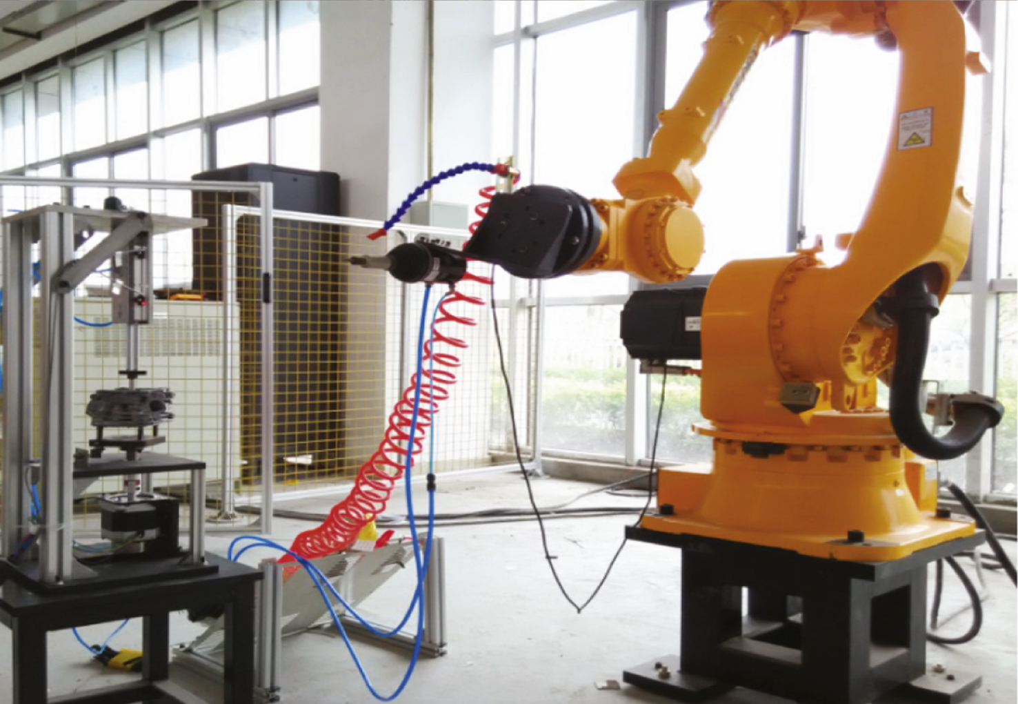
Fig.2
The traditional PID based on position feedback.
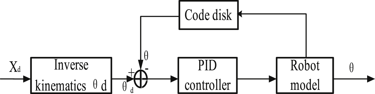
Fig.3
The fuzzy PID algorithm flow chart.
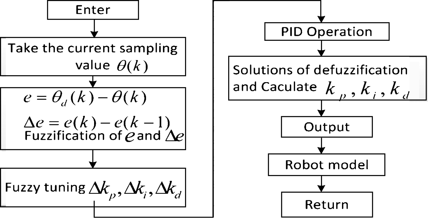
Fig.4
Membership function curves of e and ec.
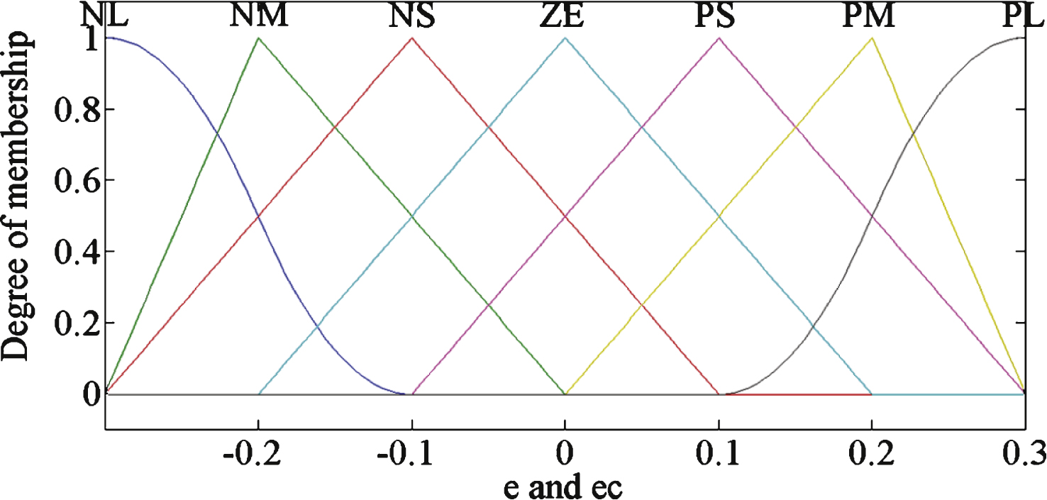
Fig.5
Membership function curves of dK p and dK i .
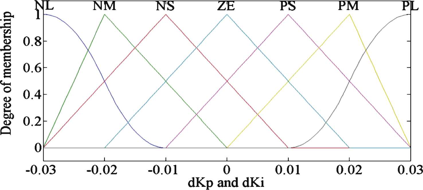
Fig.6
Membership function curves of dK d .
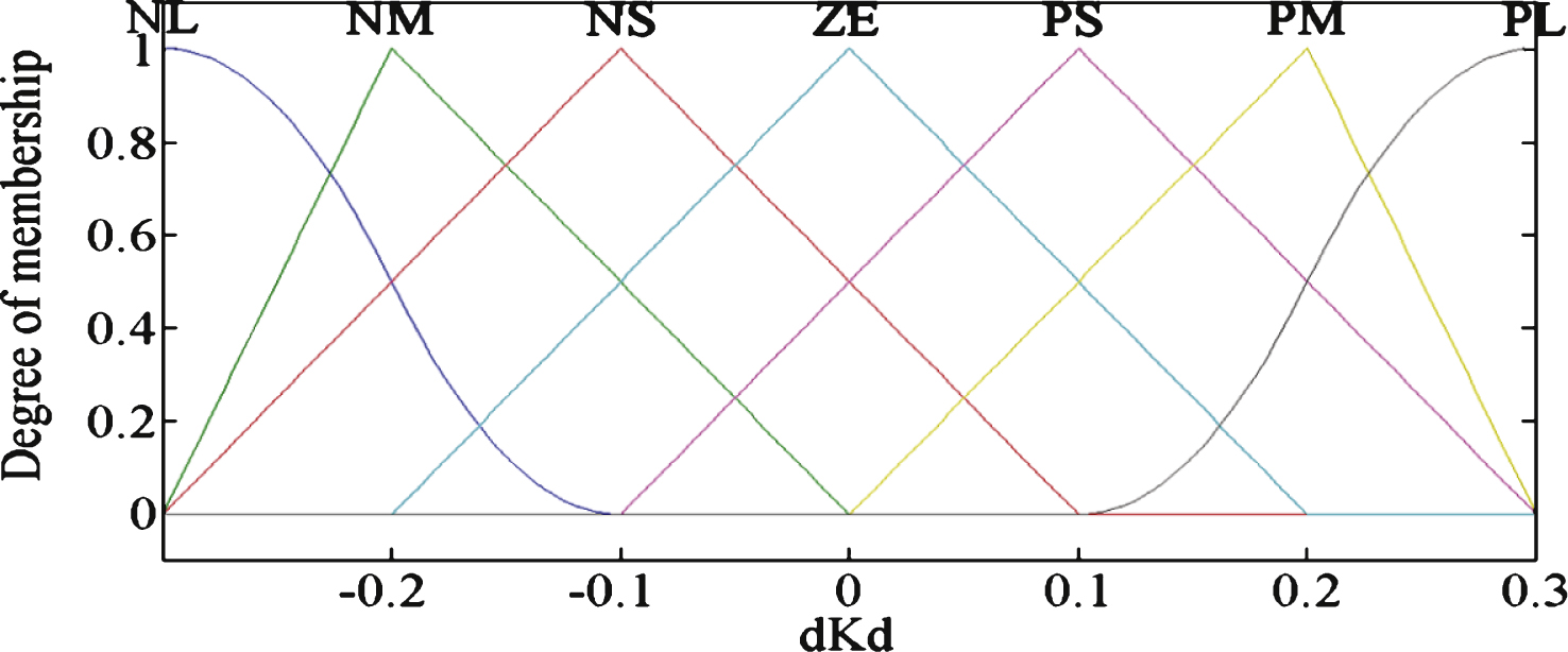
Fig.7
The fuzzy PID controller.
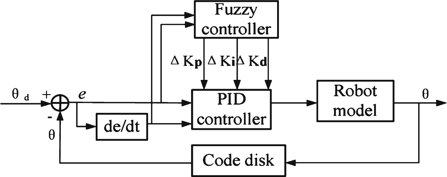
Fig.8
Working principle of the fuzzy controller.
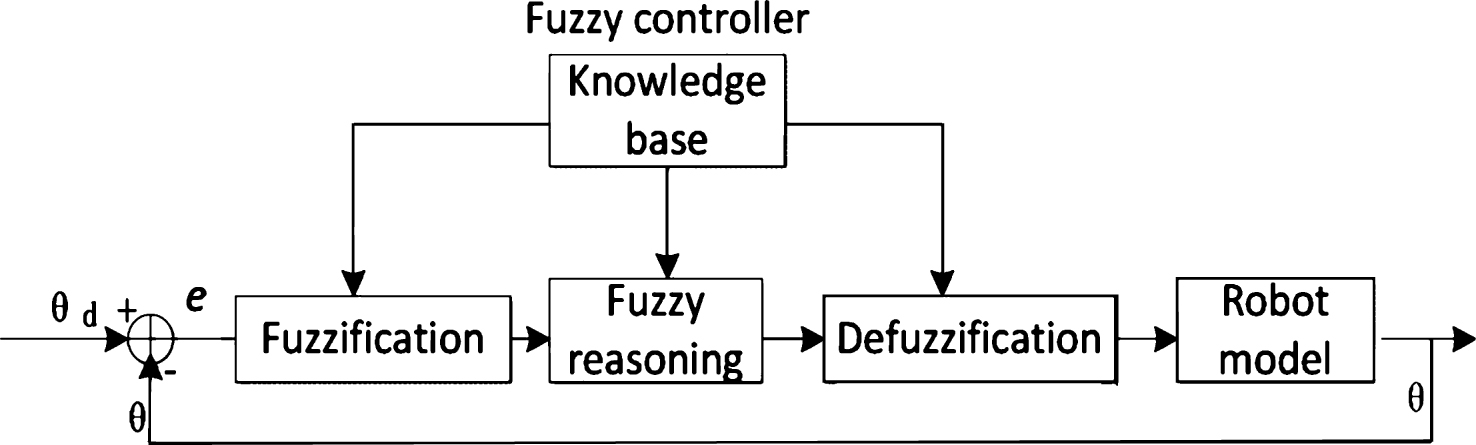
Fig.9
The orientation of the end-effector.
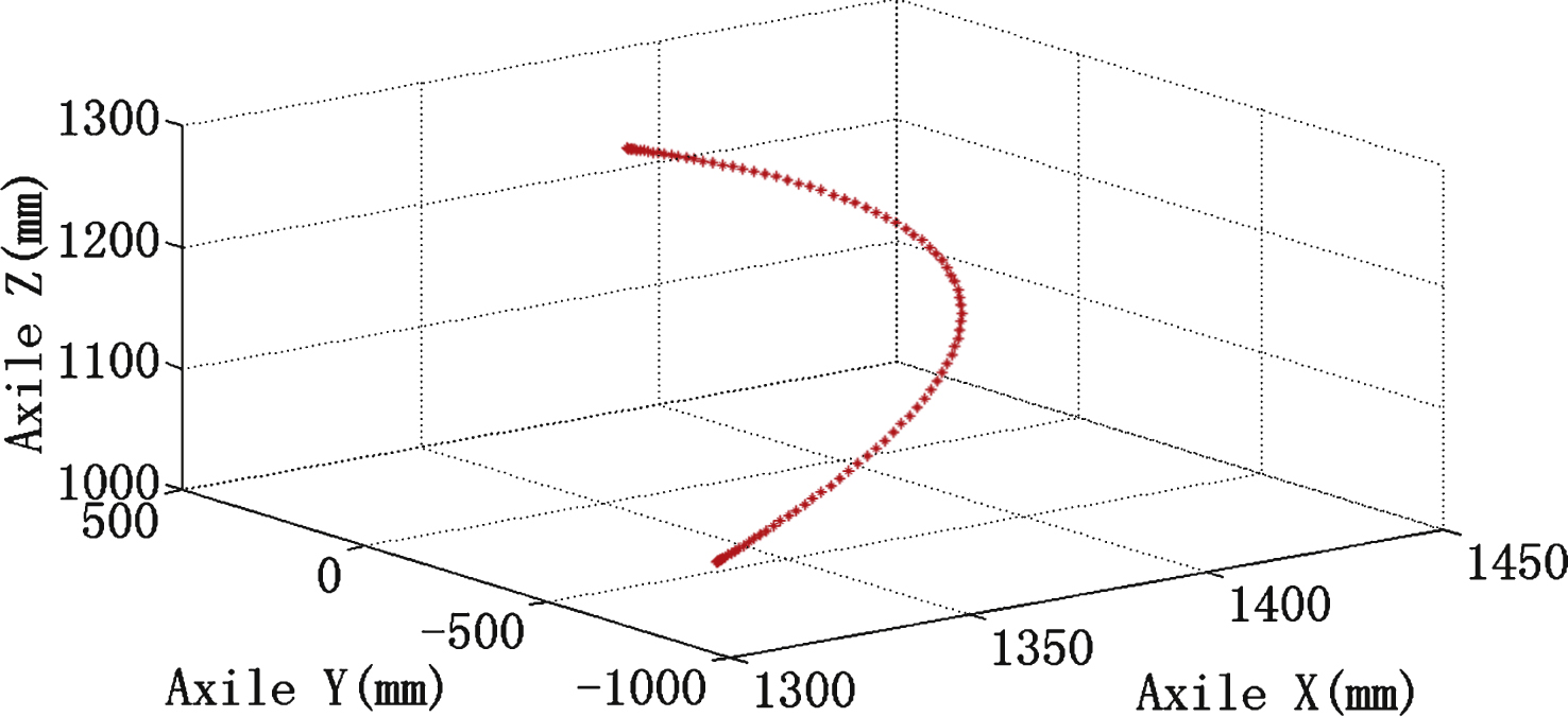
Fig.10
Joint angular based on traditional and fuzzy PID.
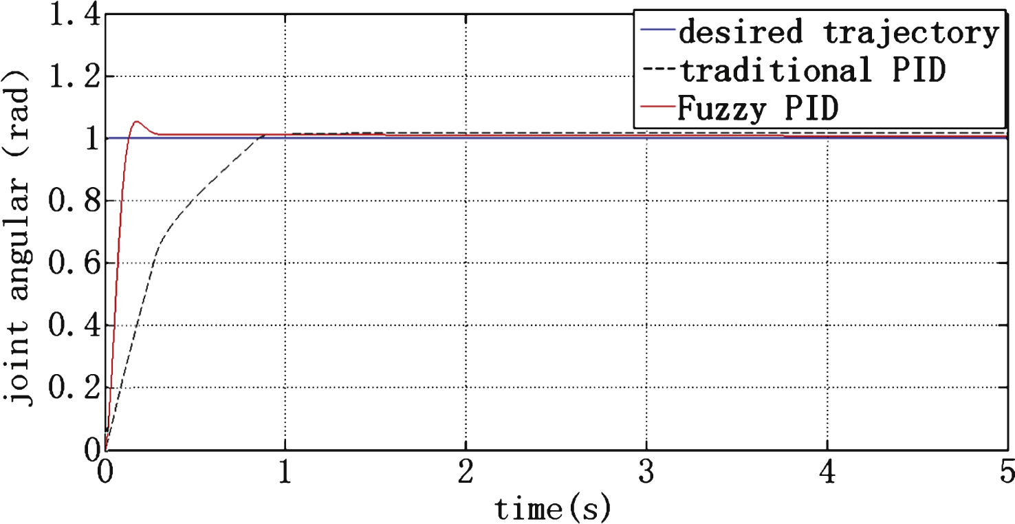
Fig.11
Error of joint angular based on traditional and fuzzy PID.
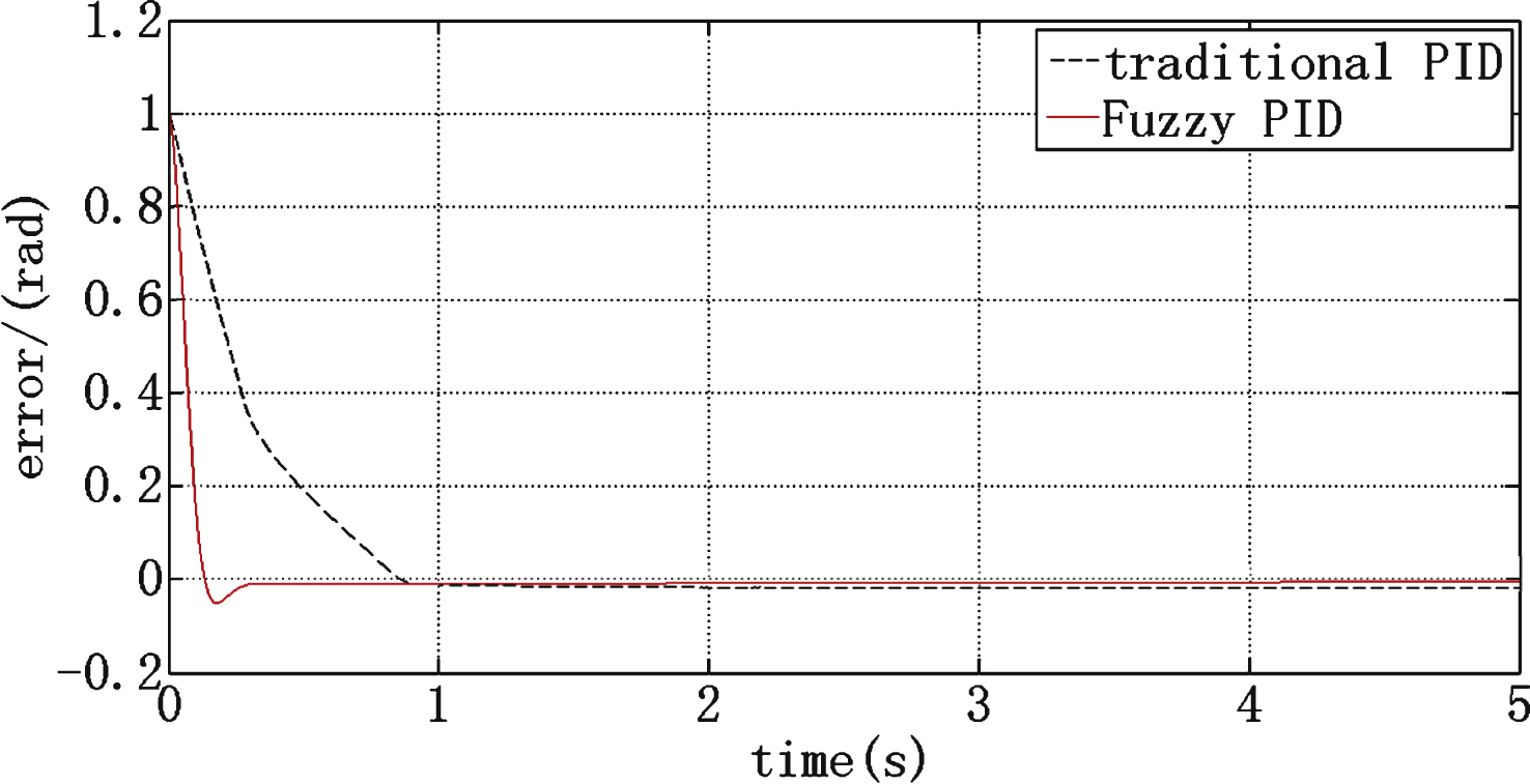
Fig.12
The value of K p based on Fuzzy PID.
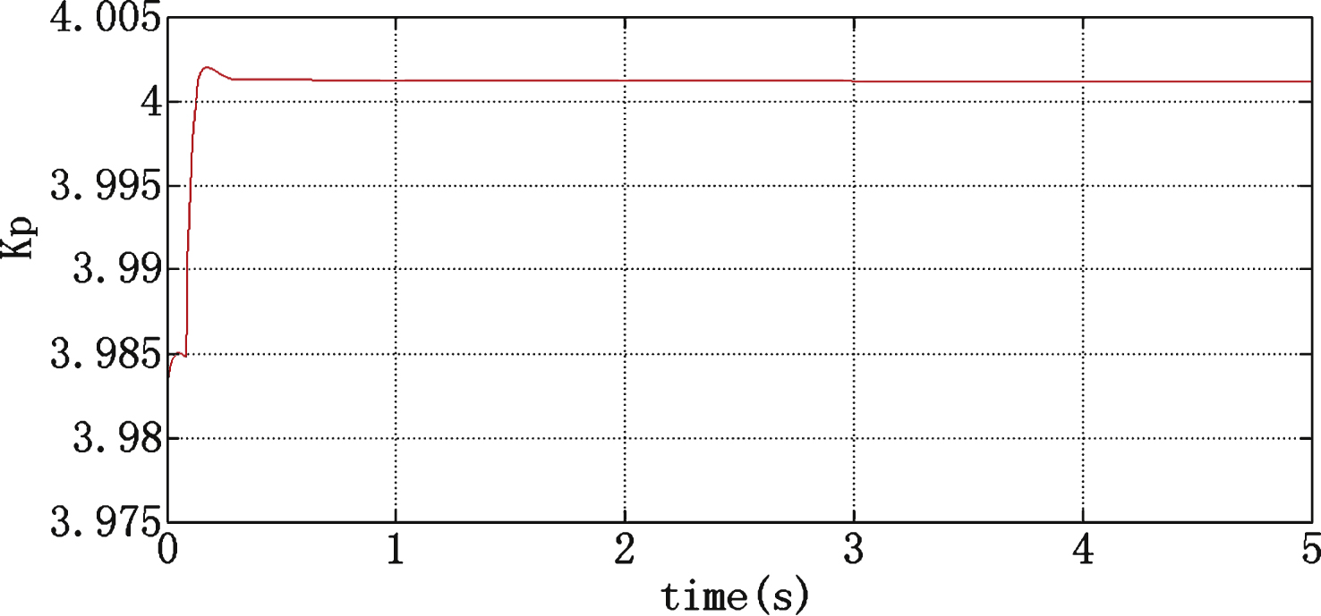
Fig.13
The value of K i based on Fuzzy PID.
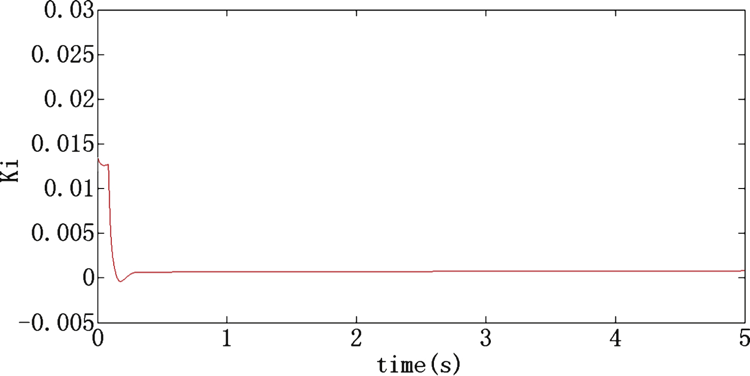
Fig.14
The value of K d based on Fuzzy PID.
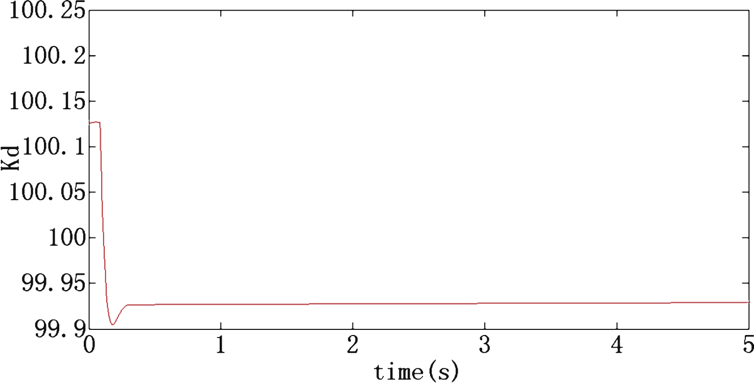
Table 1
D-H parameters of the manipulator
| Link i | Joint angle | α i-1/ | a i-1/mm | d i /mm | Range of |
| θ i /(∘) | (∘) | joint angle | |||
| 1 | θ 1 | 0 | 0 | d 1 | ±180° |
| 2 | θ 2 | –90 | a 1 | 0 | +80/–135° |
| 3 | θ 3 | 0 | a 2 | 0 | +225/–80 |
| 4 | θ 4 | –90 | a 3 | d 4 | ±360° |
| 5 | θ 5 | 90 | 0 | 0 | ±120° |
| 6 | θ 6 | –90 | 0 | 0 | ±450° |
Table 2
Fuzzy rule table for change in ΔK p
| e/ec | NL | NM | NS | ZE | PS | PM | PL |
| NL | 0.03 | 0.03 | 0.03 | 0.03 | 0.02 | 0.01 | 0 |
| NM | 0.03 | 0.03 | 0.03 | 0.03 | 0.02 | 0 | 0 |
| NS | 0.02 | 0.02 | 0.02 | 0.02 | 0 | 0.01 | 0.01 |
| ZE | 0.02 | 0.02 | 0.01 | 0 | –0.01 | –0.01 | –0.01 |
| PS | 0.01 | 0.01 | 0 | –0.02 | –0.02 | –0.02 | –0.02 |
| PM | 0.01 | 0 | –0.01 | –0.02 | –0.02 | –0.02 | –0.03 |
| PL | 0 | 0 | –0.02 | –0.02 | –0.02 | –0.03 | –0.03 |
Table 3
Fuzzy rule table for change in ΔK i
| e/ec | NL | NM | NS | ZE | PS | PM | PL |
| NL | –0.03 | –0.03 | –0.02 | –0.02 | –0.01 | 0 | 0 |
| NM | –0.03 | –0.03 | –0.02 | –0.01 | –0.01 | 0 | 0 |
| NS | –0.03 | –0.02 | –0.01 | –0.01 | 0 | 0.01 | 0.01 |
| ZE | –0.02 | –0.02 | –0.01 | 0 | 0.01 | 0.02 | 0.02 |
| PS | –0.02 | –0.01 | 0 | 0.01 | 0.01 | 0.02 | 0.03 |
| PM | 0 | 0 | 0.01 | –0.02 | 0.02 | 0.03 | 0.03 |
| PL | 0 | 0 | 0.01 | 0.02 | 0.02 | 0.03 | 0.03 |
Table 4
Fuzzy rule table for change in ΔK d
| e/ec | NL | NM | NS | ZE | PS | PM | PL |
| NL | 0.1 | –0.1 | –0.3 | –0.3 | –0.3 | –0.2 | 0.1 |
| NM | 0.1 | –0.1 | –0.3 | –0.2 | –0.2 | –0.1 | 0 |
| NS | 0 | –0.1 | –0.2 | –0.1 | –0.1 | –0.1 | 0 |
| ZE | 0 | –0.1 | –0.1 | –0.1 | –0.1 | –0.1 | 0 |
| PS | 0 | 0 | 0 | 0 | 0 | 0 | 0 |
| PM | 0 | 0.1 | 0.1 | 0.1 | 0.1 | 0.1 | 0.3 |
| PL | 0.3 | 0.2 | 0.2 | 0.2 | 0.1 | 0.1 | 0.3 |

