Equational approach to argumentation networks

Gabbay, D.M.

doi:10.1080/19462166.2012.704398

Equational approach to argumentation networks

Issue title: A Special Issue on an Equational Approach to Argumentation with a Foreword from Johan van Benthem

Article type: Research Article

Affiliations: [a] Department of Computer Science, Bar-Ilan University, 52900, Ramat-Gan, Israel | [b] Department of Informatics, King's College London, Strand, London, WC2R 2LS, UK | [c] Computer Science and Communications, Faculty of Sciences, 6, rue Coudenhove-Kalergi, L-1359, Luxembourg, Luxembourg

Correspondence: [*] E-mail: [email protected]

Keywords: argumentation networks, equational approach, support in argumentation, time-dependent networks, higher level attacks, numerical argumentation

DOI: 10.1080/19462166.2012.704398

Journal: Argument & Computation, vol. 3, no. 2-3, pp. 87-142, 2012

Received 19 April 2011

Accepted 15 June 2012

Published: 1 September 2012

Get PDF

Abstract

This paper provides equational semantics for Dung's argumentation networks. The network nodes get numerical values in [0,1], and are supposed to satisfy certain equations. The solutions to these equations correspond to the “extensions” of the network. This approach is very general and includes the Caminada labelling as a special case, as well as many other so-called network extensions, support systems, higher level attacks, Boolean networks, dependence on time, and much more. The equational approach has its conceptual roots in the nineteenth century following the algebraic equational approach to logic by George Boole, Louis Couturat, and Ernst Schroeder.

1.Introduction

This paper expands on our equational ideas introduced in (2009b, pp. 246–251). A short introduction to the results of this paper appears in Proceedings of ECSQARU’11, Springer LNAI Series, see Gabbay (2011).

This section introduces the ideas involved in the paper one by one through several subsections.

To achieve our goal, as outlined in Section 1.1, we adopt an equational approach, going back to the nineteenth century way of doing logic.

The equational approach has its conceptual roots in the nineteenth century following the algebraic equational approach to logic by Boole (1847), Couturat (1914), and Schröder (2000).

The equational algebraic approach was historically followed, in the first half of the twentieth century, by the Logical Truth (Tautologies) approach supported by giants such as G. Frege, D. Hilbert, B. Russell, and L. Wittgenstein. In the second half of the twentieth century, the new current approach has emerged, which was to study logic through it consequence relations, as developed by A. Tarski, G. Gentzen, D. Scott, and (for non-monotonic logic) D. Gabbay.

1.1.Aims of this paper

We have several good reasons for writing this paper.

(1) To provide a general computational framework for Dung's argumentation networks; a framework in which the logical aspects, computational aspects, and the conceptual aspects involved in Dung's original proposal can be isolated, highlighted, and analysed, and thus paving the way for orderly responsible generalisations.
The logical aspects involve the question of what is the logical content of an argumentation network and what inferences we can draw from it, see Gabbay (2009a) and our most recent paper (Gabbay). The computational aspects have to do with viewing the abstract argumentation networks as directed graphs or as finite models with binary relations on them and various algorithms for extracting subsets of such graphs or models. See, for example, Gabbay and Szalas (2009) on annotation theories. The conceptual aspect is the reason behind the computation, involving concepts such as conflict-free sets, admissibility, and a variety of extensions. See Caminada's conceptual survey slides (Caminada and Wu 2011) and especially slide 19.
At present, Dung's networks are generalised in many ways by many capable researchers. Unfortunately, we have no general meta-level approach which the community can use for guidance and comparison.
(2) To generalise Dung's argumentation networks in a natural way and connect and compare it with other network communities, such as neural nets, Bayesian nets, biological–ecological nets, logical, labelled deductive nets, and so forth. See Baroni, Giacomi, and Guida (2005), Barringer and Gabbay (2010), Barringer, Gabbay, and Woods (2005, 2008).
These networks have a different conceptual base but they look like abstract argumentation networks, i.e. they are directed graphs. We manipulate the graphs differently because they come from different applications. So, the question to ask is whether we can we find common ground (such as an equational approach to such graphs) which will bring the applications together at least on the formal mathematical side?
(3) To introduce in a natural way, various meta-operations on networks such as distributed networks (modal logic), time dependence, and fibring which exist in other types of networks and logics.
(4) To connect with pure mathematics, numerical analysis, and computational algebra. We will focus on Dung abstract argumentation semantics, although we also touch on some other semantics such as CF2 semantics in Gabbay (2012a).

The rest of this introductory section will explain the ideas of this paper through examples and discussion and later sections will develop the mathematical machinery involved.

Dung's (1995) argumentation networks have the form (S, R_A), where S is a set of arguments, which for the current purposes we assume to be finite, and R_A is a binary attack relation on S. We are interested in subsets E of S of arguments which are admissible, that is self-defending and conflict free, namely:

(1) E is conflict free, namely for no x, y in E do we have that xR_Ay.
(2) E defends each of its elements: whenever for some x, we have xR_Ay and y is in E, there is some z in E defending y, i.e. we have z R_Ay. (E is self-defending.)
(3) E is complete if E contains all the elements it defends.

The smallest such complete E is called the grounded extension, a maximal E (there may be several different such maximal sets) is called a preferred extension, and if we are lucky, we may also have a stable extension E, namely one which attacks anything not on it.

Such extensions are perceived as indicating coherent logical positions which can defend themselves against attacks.

See Caminada and Gabbay (2009) and Gabbay and Szalas (2009) for surveys. The above set of definitions is the original set theoretic way of introducing extensions. There is another very useful equivalent way of defining extensions, using the Caminada labelling, see Caminada and Gabbay (2009) for a survey. The Caminada labelling is the approach compatible with our equational approach. It is described in the next subsection and it is the approach we are going to work with.

1.2.The conceptual vs. computational distinction

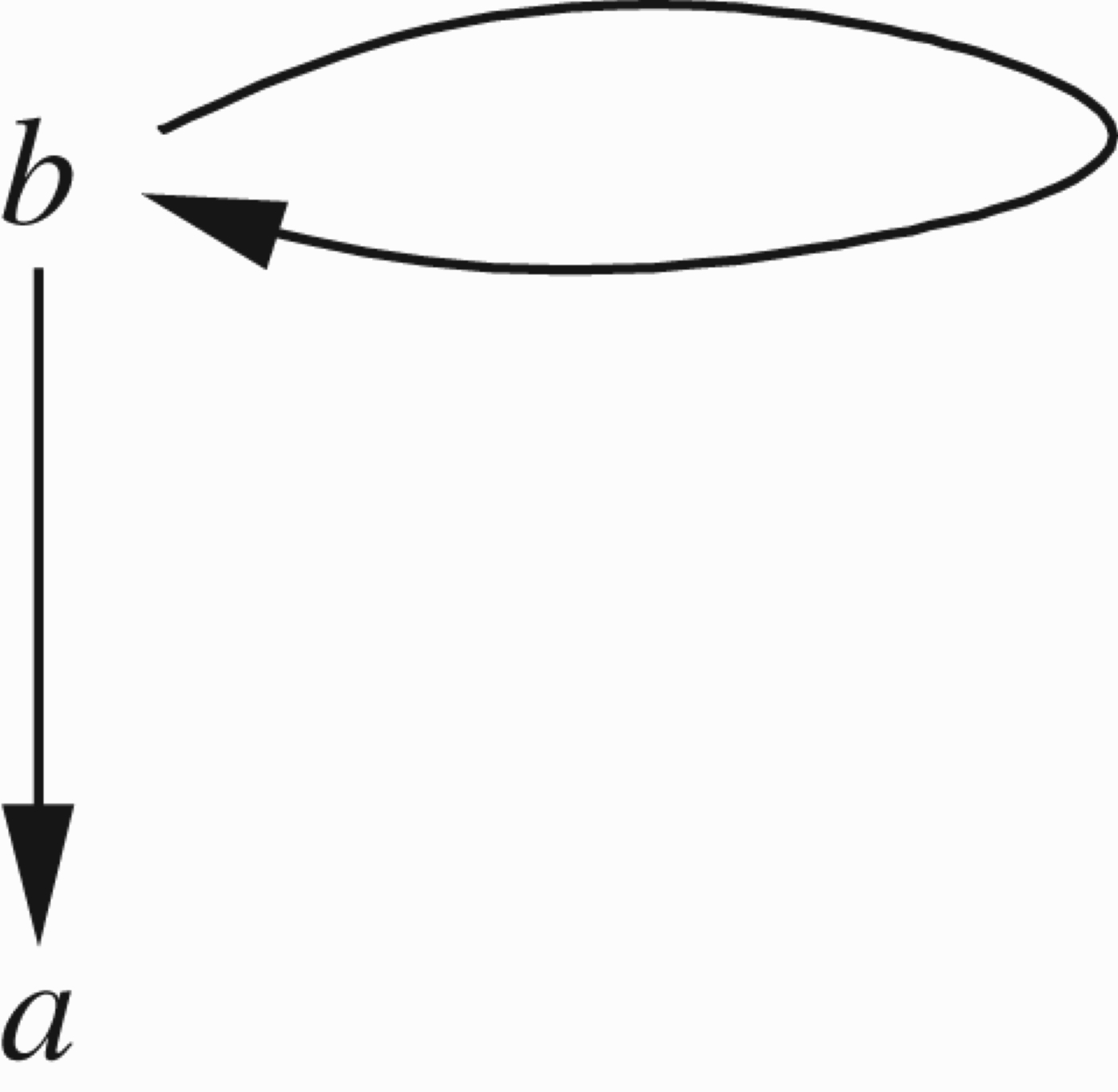
Consider the network of Figure 1

Figure 1.

A simple network.

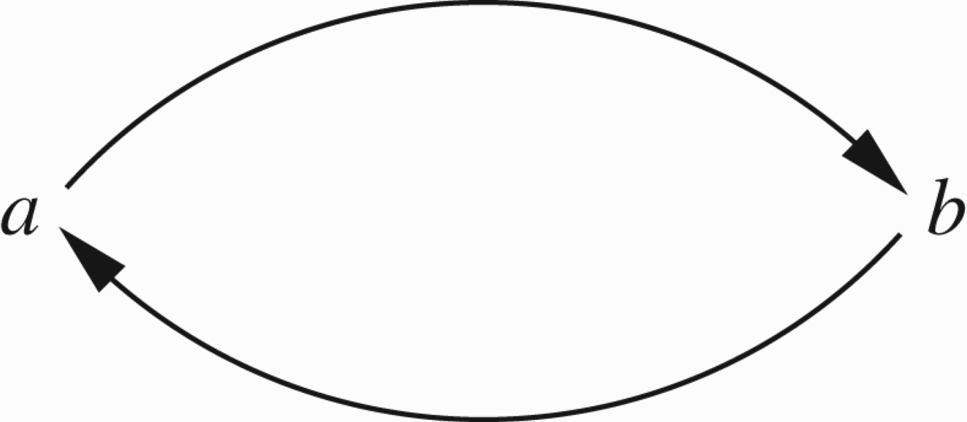
This network has two nodes S={a,b} and the attack relation R_A is described by the singel arrow “→”. We have

RA={(a,b),(b,a)}.

We follow Caminada (see survey in Caminada and Gabbay 2009) and describe three extensions:

E0={a=b=undecided},E1={a=in,b=out},E2={a=out,b=in}.

The rules governing the assignment of these values are the Caminada conditions:

Caminada conditions:

(C1) If a= in and a attacks b then b= out.
(C2) If all attackers x_i of b are out (or if there are no attackers) then b= in.
(C3) If all attackers x_i of b are either out or undecided with at least one such attacker is undecided then b= undecided.

By looking at a Dung extension E, we are saying two things:

(1) Computational statement: Assign values from <texlscub>in, out, undecided</texlscub> to all nodes in such a way that the above connections are observed.
(2) Conceptual statement: Let
Ein={x|x=in},
then we are saying that E_in is a set of arguments which is conflict free and represents a a coherent position that one can take in adopting the arguments in E_in, a position which is able to defend itself.

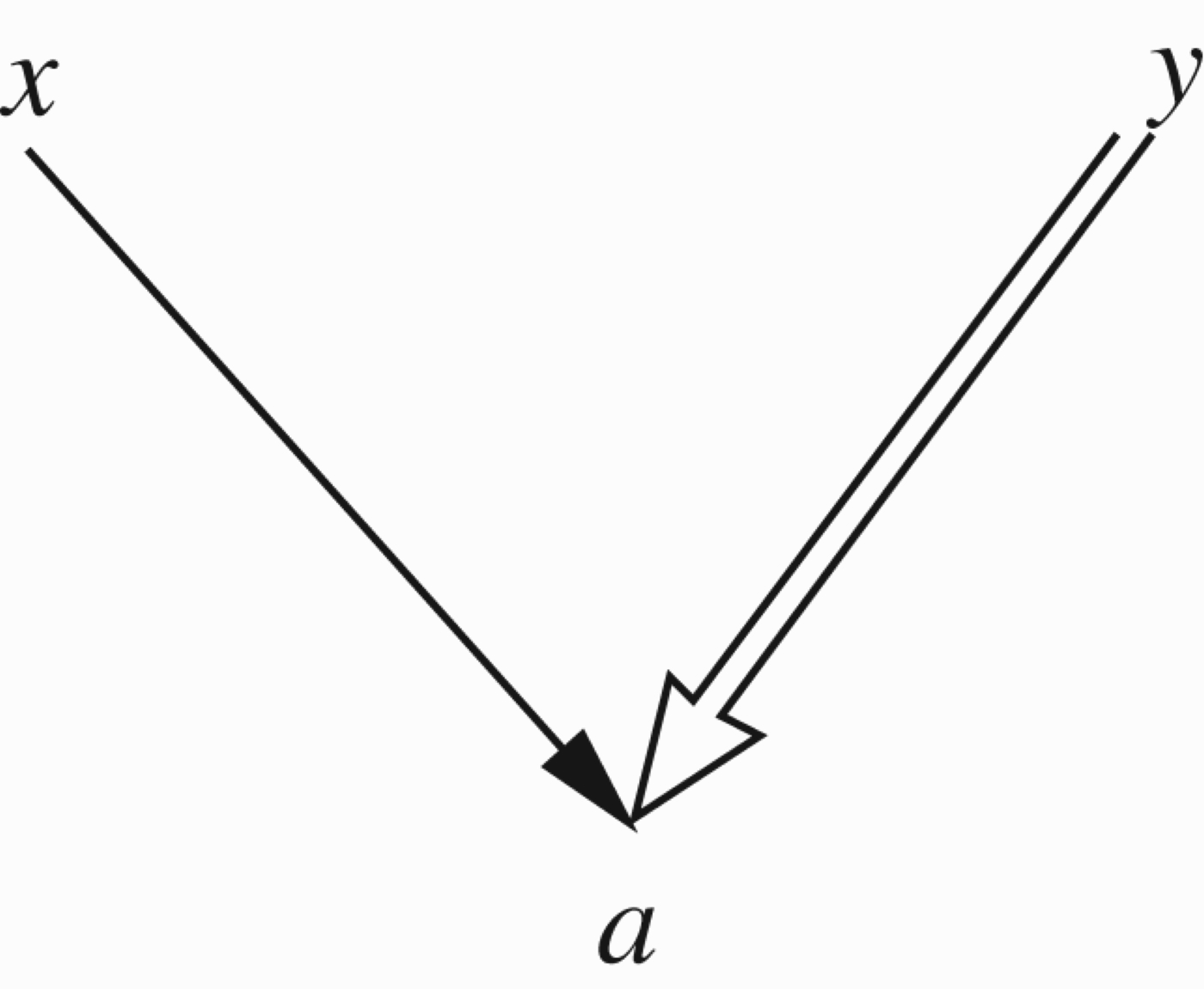
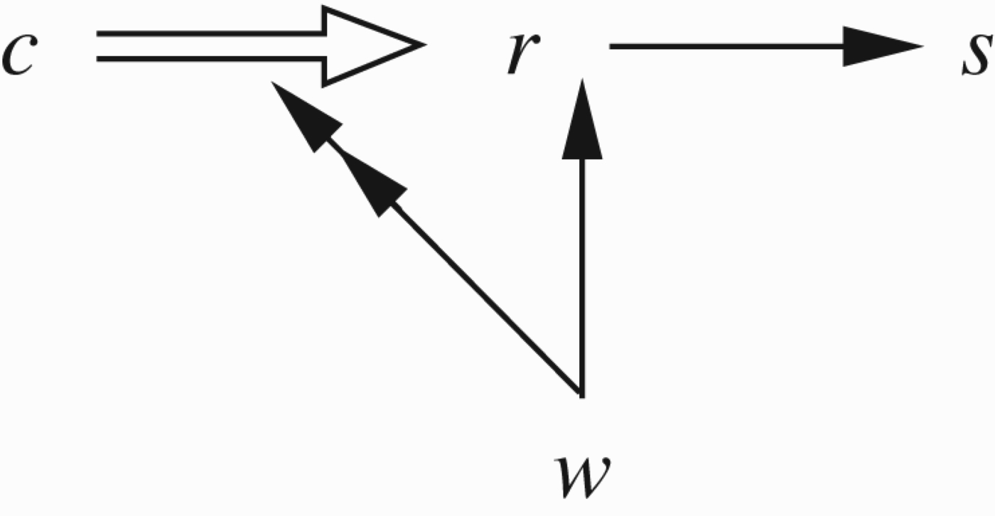
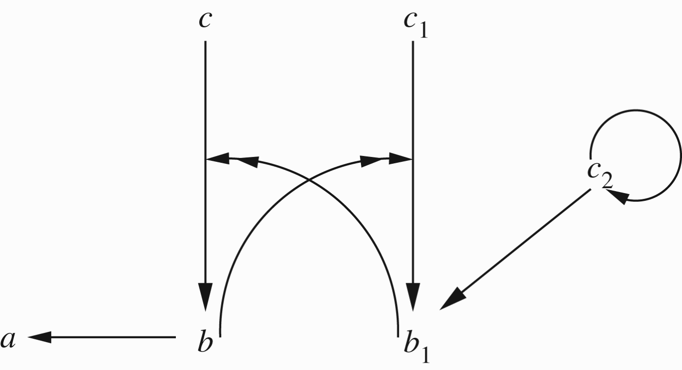
Now consider Figure 2, where we add a third element and add the new relation of support R_S, indicated by the double arrow.

Figure 2.

Adding support.

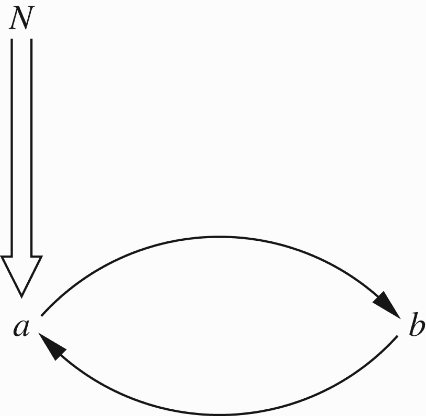
We have S={N,a,b}. RA={(a,b),(b,a)} and the support relation RS={(N,a)}. N is a special element for providing support.

We now have two problems in this new expanded network with support.

(1) Computational problem: How to assign values <texlscub>in, out, undecided</texlscub> or possibly additional labels such as weakly undecided, almost in, possibly out, etc.
(2) Conceptual problem: Extend conceptual meaning to “support” in the network. In other words, what do we mean by support. Of course, our conceptual analysis will influence what labels we use in the computational approach.

The answer to (1) is to extend the algorithm governing the assignment of values <texlscub>in, out, undecided, and other values</texlscub> to cover cases of support.

The answer to (2) is to modify the network to a new network by some conceptual considerations, which take into account of the support relation.

This can be done by modifying the notion of extension or the notion of attack or both.

Let us, by way of example, offer a minimalistic conceptual analysis of support, reading support as “endorse”. If x supports y, then x does not give more strength to the argument y, but only shares its fate, having endorsed it. Let us see what we can offer as a corresponding computational approach.

The computational aspect can be solved, for example, by keeping within the labels <texlscub>in, out, undecided</texlscub>, and by adding new rules (N1) and (N2).

(N1) If a supports b and a= out then b is out.
(N2) If a supports b and b= in then a= in.

Modify (C2) to say

(NC2) If all attackers x_i of b are out (or if there are no attackers) and if b does not support any y then b= in.

Another possibility of understanding support is as a licence for attack and defence. Here, we are really adding strength to the supported node. We can declare, for example, one of the following:

(Q1) A supported node cannot be attacked. (This reminds us of Bench-Capon's (2003) value-based networks.)
(Q2) A node which is not supported cannot attack. (See, for example, Oren, Reed, and Luck 2010).

The effect of (Q2) is to cancel the arrow b→a.

We thus get the following:

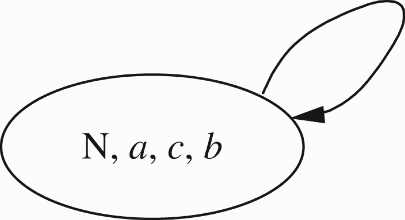
(i) If we adopt (N1), (NC2), and (N2), we get the following extensions in Figure 2:
E0={N=in,a=b=undecided},E1={N=in,a=in,b=out},E2={N=out,a=out,b=in}.
We can, of course, make all kinds of other distinctions about points which support and there is an extensive literature on this. See, for example, Boella, Gabbay, van der Torre, and Villata (2011b, 2010).
The above is just an example to explain the computational vs. conceptual aspects distinctions, see Section 3 for the analysis of support.
(ii) If we adopt (Q1) then Figure 2 is reduced to Figure 3.
(iii) If we adopt (Q2) then Figure 2 is again reduced to Figure 3, but for a different reason. (Q2) does not allow b to attack anything and (Q1) does not allow b to attack a but it can attack other points.

Figure 3.

Simplifying Figure 2.

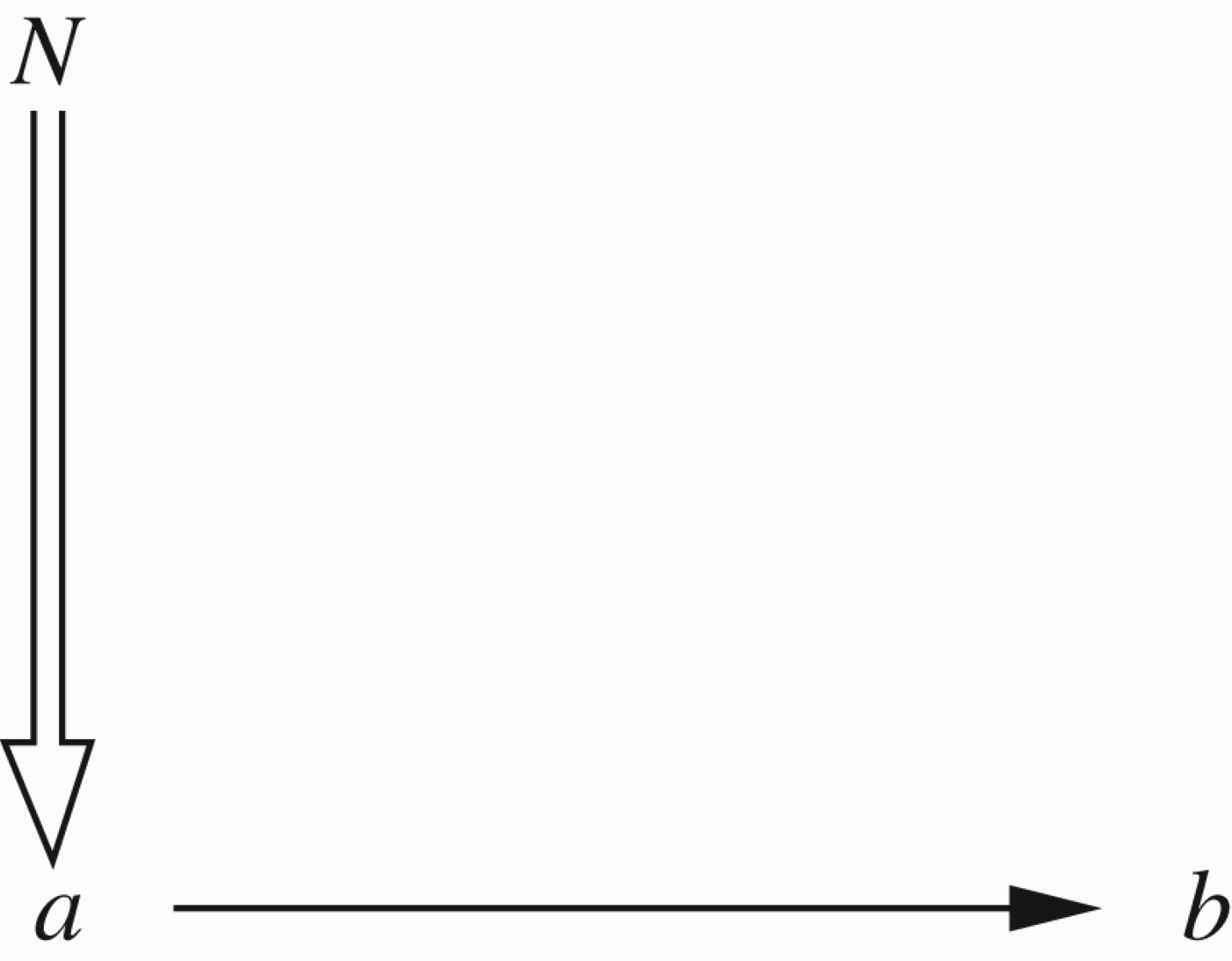
We still need computational principles for Figure 3, though in this simple figure the only option is E₁.

1.3.Equational examples

This subsection is intended to motivate the formal equation section, Section 2. We give here several examples of the equational approach.

Let (S, R_A) be a Dung network. So RA⊆S2 is the attack relation. We are looking for a function f:S↦[0,1] assigning to each a∈S a value of 0⩽f(a)⩽1 such that the following holds.

(1) (S,RA,f) satisfies the following equations for some family of functions {ha},a∈S:
- (a) If a is not attacked (i.e. ¬∃x(xRAa)) then f(a)=1.
- (b) If x1,…,xn are all the attackers of a (i.e. ⋀i=1nxiRAa∧∀y(yRAa→⋁i=1ny=xi)) then we have that f(a)=ha(f(x1),…,f(xn)).
Let us take, for example, the same ha=h for all a and let
h(f(x1),…,f(xn))=∏i=1n(1−f(xi)).
We shall call the above equation Eqinverse. We shall define other possible equations later on.
Thus, we get
Eqinverse for the function f:
f(a)=∏i=1n(1−f(xi)).
(2) For any (S,RA,f), there exists a Caminada labelling of (S, R_A), such that
λ(a)=in,iff(a)=1,out,iff(a)=0,undecided,if0<f(a)<1.

The equation

f(a)=∏i=1n(1−f(xi))

ensures that:

If one of x_i (x_i are the attackers of a) is in then a is out.

If all the attackers are out then a is in.

If at least one of the attackers of a is undecided and none of the attackers of a are in then a is undecided.

The question remaining to be asked is the following:

If we have a Caminada labelling, can we find a function f solving the Eqinverse equations which correspond to this Caminada labelling as in (2) above? The answer is negative, as Examples 1.7 and 1.11 show.

Let us now give a formal definition.

Definition 1.1

Definition 1.1Possible equational systems

Let (S, R_A) be a networks and let a be a node and let x1,…,xn be all of its attackers.

We list below several possible equational systems, we write Eq(f) to mean the equational system Eq applied to f:

(1) Eqinverse(f)
f(a)=∏i(1−f(xi)).
(2) Eqgeometrical(f)
f(a)=[∏i(1−f(xi))][∏i(1−f(xi))+∏if(xi)].
We call this equation Eqgeometrical because it is connected to the projective geometry Cross Ratio, see Barringer et al. (2005).
(3) Eqmax(f)
f(a)=1−max(f(xi)).
We shall see the difference in the examples. In fact, we shall see that this new function gives exactly the Caminada labelling.
(4) Eqsuspect(f)

Let us further introduce a fourth system of equations which we call Eqsuspect(f):

ha(f(x1),…,f(xn))=∏i(1−f(xi)),if¬aRAaholds

and

ha(f(x1),…,f(xn))=f(a)∏i(1−f(xi)),ifaRAaholds.

Example 1.2

Consider Figure 1 again.

Let

f(a)=α.f(b)=β.

The equations are (using Eqinverse, or indeed any other option, they are all the same on this example):

(1) α=1−β.
(2) β=1−α.

If we choose α, this fixes β.

For α=1, we get β=0. For α=0, we get β=1. For 0<α<1, we get 0<β<1.

We thus get the three extensions, if we read any value strictly between 0 and 1 as undecided.

E0={a=b=undecided},E1={a=in,b=out},E2={a=out,b=in}.

Example 1.3

Consider Figure 4. Here, the equation is (for f(a)=α, and all Equational options except Eqsuspect):

α=1−α.

so α=12.

Thus, the extension is

{a=undecided}.

In the case of Eqsuspect, the equation is α=α(1−α) and the solution is α=0.

Example 1.4

Consider Figure 5

Let f(a)=α,f(b)=β and f(c)=γ.

The equations are under all options

(1) α=1−γ.
(2) β=1−α.
(3) γ=1−β.

From 1 and 3, we get α=β and from 1 and 2, we get α=γ and so α=β=γ=12.

The extension is {a=b=c=undecided}.

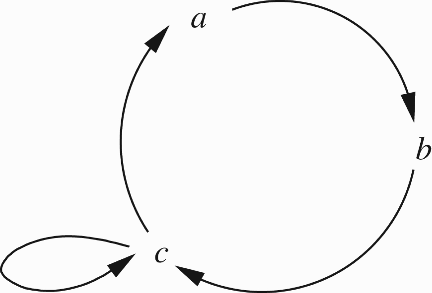
Example 1.5

Consider Figure 6. Again we get, for f(a)=α,f(b)=β,f(c)=γ.

Let us use the set Eqinverse(f):

(1) α=1−γ.
(2) β=1−α.
(3) γ=(1−β)(1−γ).

From (1) and (2), we get

(4) γ=β.

Therefore, from (3) we get

(5) γ=γ(1−γ).
Therefore,
(6) γ=0,α=1,β=0.

This gives us the extension

{a=in,b=out,c=out}.

Note that this corresponds to condition 2 on f. Since the only Dung extension says I do not know (undecided) on {a,b,c}, any value given by f is compatible.

Let us now consider EqSuspect. The equations are

(1) α=1−γ.
(2) β=1−α.
(3) γ=γ(1−β)(1−γ).

From (1) and (2), we get

(4) γ=β.

Therefore, from (3) we get

γ=γ(1−γ)(1−γ).

The only solution is γ=0, and therefore β=0,α=1.

We now consider Eq_max. We get

(1) α=1−γ.
(2) β=1−α.
(3) γ=1−max(β,γ).

From (1) and (2), we get

(4) γ=β.

From (3), we get

(5) γ=1−γ.

Therefore, γ=12 and hence α=β=12.

Let us now check Eqgeometrical. We get

(1) α=1−γ.
(2) β=1−α.
(3) γ=(1−γ)(1−β)/((1−γ)(1−β)+βγ).

(1) and (2), we get

(4) β=γ.

and from (3), we get

(5) γ=(1−γ)2/((1−γ)2+γ2).

Therefore

(6) γ(1−γ)2+γ3=(1−γ)2

and hence

γ3=(1−γ)3.

The only solution is γ=12 and hence α=β=12.

Remark 1.6

Actually, there is a rationale to what is happening in the previous Example 1.5. Consider the network of Figure 6.

Start by assuming a=in. Then b is unambiguously out. Now the question of whether c is in or out is not clear cut. We may wish to adopt a new policy in this case, different from the traditional one. c is not attacked by b but it does attack itself. So our new policy can consider whether to make c out or undecided. It cannot be in. That c is out is the best solution.

The other alternative, that a is out, entails b is in, therefore certainly c is out and so a must be in, a contradiction.

So the best solution is a=in, b=out, and c=out, as suggested by the equational network. Although the equational approach need not be compatible with Dung's approach, it being different and new, it is worth noting that in this case, it does not contradict the Dung extension which says all undecided, but further refines it, as we have argued.

Let us look at the situation in terms of admissible extensions. The set E={a} is conflict free but not admissible because a is attacked by c and there is nothing in E which attacks c. This is the Dung concept of admissible.

Suppose we introduce and use two new concepts:

• c is Suspect if c attacks itself or possibly part of a loop of attacks which make it Suspect (the details needs to be worked out).
• E is Suspect–Admissible if whenever a in E is attacked by c then either c is Suspect or E attacks c.

By exploiting the right concepts of Suspect–Admissible and Suspect, we might be able to find a qualitative set theoretic non-equational definition of extensions corresponding to our equational extensions.

Example 1.7

Consider Figure 7 and use the set Eqinverse(f)

We have, under Eqinverse

(1) α=1−β.
(2) β=(1−α)·(1−β).

Thus, from (1) and (2) we get

(3) β=β(1−β).

So β=0,α=1.

So we get the extension {a=1,b=0}.

It is clear from Equation (3) that there is no way of letting 0<α<1 and 0<β<1 (i.e. making a and b undecided) and satisfying the Eqinverse equations for this example. Again, see Remark 1.6.

Let us consider the other Eq options.

Under Eq_max, we get

α=β=12.

Under Eqsuspect, we get the equations

(1) α=1−β.
(2) β=β(1−α)(1−β).

From (1) and (2), we get

(3) β=β2(1−β)

the only solution is β=0.

Under Eqgeometrical, we get the equations

(1) α=1−β.
(2) β=(1−α)(1−β)/((1−α)(1−β)+αβ).

From (1) and (2), we get

(3) β=β(1−β)/(β(1−β)+(1−β)β).

We get β=12 and hence α=12.

Example 1.8

Consider Figure 8 and use Eqinverse.

Here, we have

(1) α=(1−α)(1−β).
(2) β=(1−α)(1−β).

Therefore, α=β and we have

α=(1−α)2,α2−3α+1=0,α=1.5±1.25.

Only the −√1.25 makes sense as α must be in [0, 1]. So α≈0.382,β=0.382. Note that while Dung says undecided, f is very specific about a and b.

Note that Eq_max and Eqgeometrical give value ½ to all nodes.

We now examine the case of Eqsuspect. The equations are

(1) α=α(1−α)(1−β).
(2) β=β(1−α)(1−β).

The only solution is α=β=0.

Example 1.9

Example 1.9Caminada labelling and the Max function

We saw in Examples 1.5 and 1.7 and in Remark 1.6 that the functions of Eqinverse(f) do not give all possible Caminada labellings, but only some of them. To every function f, there corresponds a Caminada labelling but some Caminada labelling may not have a corresponding f. So we ask is there a system of equations which gives exactly the Caminada labelling? The answer is yes, it is the function Eqmax(f). Let us check what we get for the network of Figure 6 under this labelling. The equations are:

(1) α=1−γ.
(2) β=1−α.
(3) γ=1−max(γ,β).

The solution to these equations is α=β=γ=12.

We get the same agreement for Example 1.7. We shall prove a general theorem in the next section.

Example 1.10

Let us do another example using all four options for equations, namely Eqgeometrical,Eqinverse,Eqmax, and Eqsuspect.

Consider Figure 9. We are looking for f solving the equations. Let f(a)=α,f(b)=β,f(c)=γ.

(I) We use Eqinverse:

The equations are

(1) α=(1−α)(1−γ).
(2) β=(1−β)(1−α).
(3) γ=1−β.

There are programs like Maple which can solve the equations of this sort and give all the solutions. We used one and got

α=1−22,β=2−1,γ=2−2.

Let's solve the equations by hand. We get from (3):

(4) β=1−γ.
(5) From (4) and (1), we get that
α=(1−α)β,α=β−αβ,α=β1+β.
Therefore
(1−α)=1−β1+β,=11+β.
(6) So from (5) and (2), we get
β=1−βl+β,β+β2=1−β,β2+2β−1=0,(β+1)2=2.
So we get
(7) β=2−1.
Hence,
(8) From (5) we get
α=2−12=1−12=1−22.
(9) From (3) we get
γ=2−2.

The interest in this case is that we are getting all kinds of values which shows that these equations are sensitive to the nature of the loops involved!

(II) We use Eq_max:

The equations are

(1) α=1−max(α,γ).
(2) β=1−max(β,α).
(3) γ=1−β.

We distinguish two cases:

Case 1: β⩾α.
Then from (2), β=1−β, i.e. β=12.
So γ=12 and from 1
α=1−max(α,12),α+max(α,12)=1.
The only way the last equation can be true is that α=12.
So β⩾α implies α=β=γ=12.
Case 2: β<α.
From (2) we get
β=1−α
and from 3 we get
α=γ.
So from 1 we get
α=1−α.
So α=12 and therefore β=γ=12.
So the final solution in this case is α=β=γ=12.

(III) We use Eqsuspect:

The equations are

(1) α=α(1−α)·(1−γ).
(2) β=β(1−β)(1−α).
(3) γ=1−β.

We check some cases.

Case 1: α=0. Then from 2, we get β=β(1−β) which forces β=0 and from 3 γ=1.
So the answer for case α=0 is that also β=0 and γ=1.
Case 2: α≠0.
Can this case arise? From 1 we get
1=(1−α)(1−γ).
This cannot hold if α>0!
Thus, the solution is α=0,β=0,γ=1.
This is compatible with Remark 1.6.

(IV) We use Eqgeometrical.

The equations are:

(1) α=(1−α)(1−γ)(1−α)(1−γ)+αγ.
(2) β=(1−α)(1−β)(1−α)(1−β)+αβ.
(3) γ=1−β.

We first note that the values α=0 or α=1 or β=0 or β=1 cannot be solutions and so in our calculations, we can divide by α or β or 1−α or 1−β.

From Equation (1), we get a contradiction if α is either 0 or 1, and from Equation (2), we get a contradiction if β is either 0 or 1.

From (3) and (1), we get

(4) α=(1−α)β/((1−α)β+α(1−β))

Solving (4) for β we get

α(1−α)β+α2(1−β)=(1−α)β,α(1−α)β+α2−α2β=(1−α)β,β(1−α−α(1−α)+α2)=α2.

Therefore, we get

(5) β=α2/((1−α)2+α2).

Therefore

1−β=(1−α)2(1−α)2+α2.

Therefore

(5a) β/(1−β)=(α/(1−α))2.

We continue. Solving (2) for α we get

(6) α=(1−β)2/((1−β)2+β2).
Therefore, 1−α=β2/((1−β)2+β2)
So
(6a) α/(1−α)=((1−β)/β)2

From (5a) and (6a), we get

(7) β(1−β)=((1−β)/β)4.
Let x=β/(1−β).
Then x is s fifth root of unity, i.e. it solves the equation
(8) x⁵−1=0.
The fifth roots of unity can be solved by radicals, the only real solution is x=1, which makes β=12 and so α=γ=12.

The other solutions are complex numbers and are not relevant to us1 1

Example 1.11

Example 1.11Comparing Eq_max and Eqinverse

We shall show that these two equational systems may not yield the same extensions. The network is described in Figure 10.

Extensions according to Eq_max.

Let us compute the equations according to Eq_max and their possible solutions.

The equations are (we write “x” instead of f(x):

(1) a=1−b.
(2) b=1−max(a,b).
(3) c=1−max(b,e).
(4) d=1−c.
(5) e=1−d.

We get From (4) and (5)

(6) c=e.

From (1) and (2), we get

(7) b=1−max(1−b,b).

The only solutions to (7) are b=0 and b=½.

Case b=0

We get from (1) that

a=1.

From (6) and (3), we get

c=1−max(0,c)

therefore

c=12.

Therefore, also d=e=12.

Case b=½

Therefore from (1)

a=12.

From (3) and (6), we get

c=1−max(12,e).

From (4) and (5), we get c=e. The only solution is therefore

c=12.

Therefore e=½ and d=½.

Summary for Eq_max

We get two extensions

(1) {a},(a=1,b=0,c=d=e=12).
(2) ϕ,(a=12,b=12,c=d=e=12).

Compare this result with Theorem 2.7.

Extensions according to Eqinverse

We now deal with Figure 10 using Eqinverse. The equations are:

(1) a=1−b.
(2) b=(1−b)(1−a).
(3) c=(1−b)(1−e).
(4) d=1−c.
(5) e=1−d.

We can have one solution with a=1. 1 yields b=0, which agrees with 2. From 3 and (5), we get c=d and from (4), we get c=½ and so d=e=12.

We now ask is there a solution with a<1? Equations 1 and 2 must agree. From 1

b=1−a.

Let us substitute in 2. We get

(1−a)=a(1−a).

Since a≠1, we can divide and get

a=1

a contradiction.

Summary of extensions for Eqinverse

We can have only one extension

{a},(a=1,b=0,c=d=e=12).

Example 1.12

Let us now introduce support into our networks. Let us consider Figure 2 again.

The computational problem in our context is simply to say what equation to give for nodes like a in Figure 2 which is also additionally supported. The conceptual problem remains the same.

Let us propose an equation for support, just as an example. Suppose we have the situation as follows:

(1) All of the attackers of node a are x1,…,xm.
(2) All the nodes supported by a are y1,…,yn.

Then, we require the following equation, obtained by modifying the Eqinverse equation:

f(a)=∏i=1m(1−f(xi))∏i=1nf(yj).

If a node x is neither attacked nor supported and it does not support anything then f(x)=1.

Let us write the equations for Figure 2.

Let f(a)=α,f(b)=β,f(N)=ν.

(1) ν=α.
(2) α=ν(1−β).
(3) β=1−α.

We get that α is arbitrary and ν=α and β=1−α.

Note that there is a principle involved here in how to obtain equations which include support from equations which include attacks. Take any equation for attacks of nodes x_i and y_j on a node a, which include the participation of the node y as an attacker. Then f(y) appears in the equation involved, say one of the equations in Definition 1.1.

Now suppose we change the role of y from attacker to supporter, then the equation changes by substituting “1−f(y)” for “f(y)” in the equation.

So the principle we used can be summarised as follows:

The support by f(y) is equivalent to the attack by 1−f(y).

1.4.More on what equations can do

Example 1.13

Example 1.13Boolean functions, Abstract dialectical framework of Brewka and Woltran 2010

The function f in (S,RA,f) can be governed by a different equation for each node. So we have, for each a∈S a different function ha. So if x_i for i=1, …, n are all the nodes linking a (i.e. x_i→a is in R_A), we have

f(a)=ha(f(x1),…,f(xn)).

For example ha can be different Boolean functions in x1,…,xn. Let ℬ_a be a Boolean expression in x1,…,xn of the form

⋁i=1k⋀j=1nεi,j,

where εi,j∈{+xj,−xj}.

Let

e(εi,j)=f(xj)ifεi,j=+xj,(1−f(xj))ifεij=−xj.

Let

ha(f(x1),…,f(xn))=1−∏i=1k1−∏j=1ne(εij).

ha implements the Boolean expression ℬ_a.

We chose basically to use Eqinverse as our basis, but we could have used other functions from Definition 1.1. The functions we chose are most appropriate for dealing with logic programming, as we shall do below.

Note that since our graph (S, R_A) is a Dung network, it comes with the convention that points which are not attacked should get the value 1.

Thus the function ha for any such point should be 1.

To render this example most general, we need to give up this convention, and regard (S, R_A) as a general directed graph.

We can of course still retain the Dung convention, in which case the Boolean equations need to respect that certain points have pre-determined value of 1.

Compare with Brewka and Woltran (2010) and Brewka, Dunne, and Woltran (2011).

Note that this type of function already appears in Barringer et al. (2005). Boolean functions are discussed in Boella et al. (2011b, 2010), where it is shown how to translate Brewka and Woltran (2010) Boolean conditions into ordinary Dung networks using methods of Gabbay (2009b). See also Example 2.11 and Remark 2.17.

Remark 1.14

Remark 1.14Order among attackers

Note that in the Boolean functions Example 1.13, the local functions ha are not symmetrical but uses some order on the attackers. By giving the attackers different names and writing a Boolean expression in them, we cannot permute the names. This should be compared with ordinary Dung networks where there is no order among the attackers.

2.Formal theory of the equational approach to argumentation networks

In this section, we formally develop our equational approach. We start with equational networks based on the unit real interval [0, 1]. We then consider Boolean equations and compare with the work of Brewka and Woltran.

Conceptually, the nodes and the equations attached to them is the network and the solutions to the equations are the complete extensions, as we have seen in the examples of Section 1.

The meaning of the real numbers attached to nodes varies from one application to another and depends on the nature of the network. If the networks describe liquid flow, then the numbers are relative capacities. If the networks describe some ecology (for example, a biological predator prey network), then the numbers represent percents of populations in equilibrium. If the network is a logical network, then the numbers are truth values.

In the case of argumentation networks, numbers strictly between 0 and 1 generally mean that the node is undecided. However, the numbers can be connected to the geometry of the network and the type of loops there are in it. We saw such examples in the previous section where we got different solutions for different loops (compare, for example, the solutions to the networks in Figures 5, 6, and 9). We still need to investigate the connection between loops and solutions, we have no theorems in this area. See, however, our discussions and examples in Gabbay (2012a,b).

Figure 4.

Self loop.

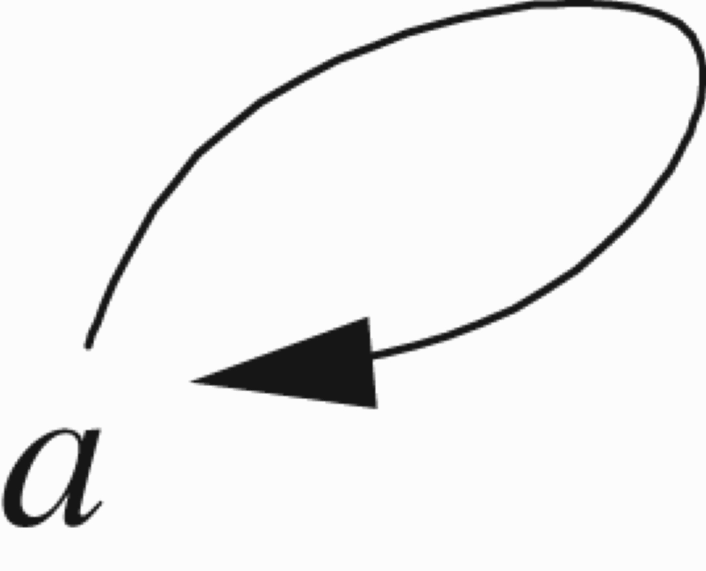
Figure 5.

Odd three loop.

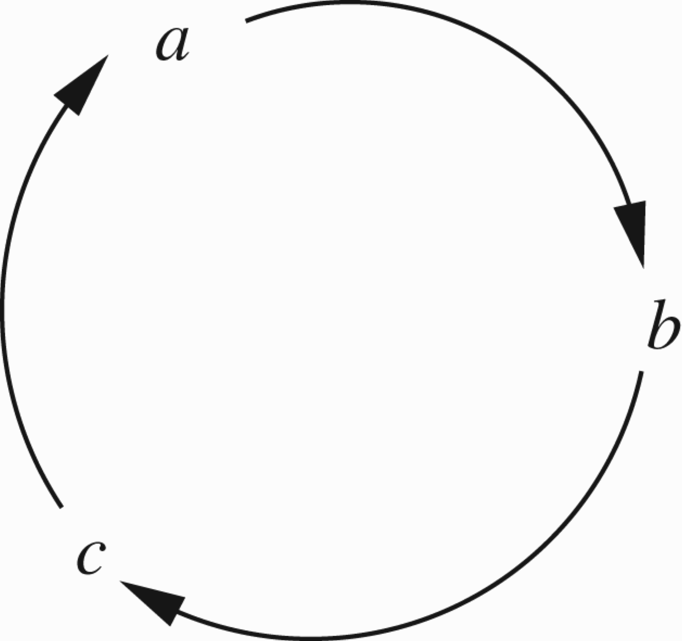
Figure 6.

Odd loop with a self looping element.

2.1.Real numbers equational networks

Definition 2.1

Definition 2.1Real equational networks

(1) An argumentation base is a pair (S, R_A) where S≠∅ is a finite or an infinite set and RA⊆S2 is a finitary relation, that is for all x in S the set {y|yRAx} is finite.
(2) A real equation function in k variables {x1,…,xk} over the real interval [0, 1] is a continuous function h:[0,1]k↦[0,1] such that
- (a) h(0,…,0)=1.
- (b) h(x1,…,1,…,xk)=0.
  Sometimes we also have condition (c) below, as in ordinary Dung networks, but not always.
- (c) h(x1,…,xk)=h(y1,…,yk), where {yj}={xi} are permutations of each other.
(3) An equational argumentation network over [0, 1] has the form (S,RA,ha), a∈S where
- (a) (S, R_A) is a base.
- (b) For each a∈S,ha is a real equation function, with the suitable number of variables k, k being the number of nodes attacking a.
- (c) If ¬∃y(yRAa) then ha≡1.
(4) An extension is a function f from S into [0, 1] such that the following holds:
- • f(a)=1 if ¬∃y(yRAa),
- • If {x1,…,xk} are all the elements in S such that x_iR_Aa, then ha is a k variable function and f(a)=ha(f(x1),…,f(xk)).

Theorem 2.2

Theorem 2.2Existence theorem, the finite case

Let (S,RA,ha),a∈S be a finite network as in Definition 2.1. Then, there exists an extension function f satisfying (4) of Definition 2.1.

Proof

Let n be the number of elements of S. For each a∈S consider ha as a continuous function from [0,1]S↦[0,1]. Note that in reality a may be attacked by only k nodes, with k possibly less than n. In this case, ha is a function of k variables, but we can consider it as a function of n variables. This is a common practice in mathematics. Let h be the continuous function from [0, 1]^S into [0, 1]^S defined component wise by h(α1,…,αn)=(ha1(α1,…,αn),…,han(α1,…,αn)).

This is a continuous function on a compact cube of n dimensional space and has therefore, by Brouwer's fixed point theorem, a fixed point (x1,…,xn)=h(x1,…,xn).

Let f be defined by f(ai)=xi. Then, we have that for each a∈S

f(a)=ha(f(a1),…,f(ak)),

where a_i are all the points in S attacking a. ▪

Remark 2.3

For Brouwer's fixed point theorem, see Wikipedia.2 2

Remark 2.4

The perceptive reader should note that Theorem 2.2 ensures that some solution “extension” exists for any continuous function assigning to each argument a value in [0, 1] on the basis of values assigned to all other arguments (the attack relation is irrelevant for the result). While this ensures that one has not to care for existence problems in defining equations, it also means that both meaningful and meaningless (in the sense that they have nothing to do with the notion of extension) equations provide some result. It is therefore an important issue to identify criteria for selecting meaningful equations for argumentation semantics. We provided some interesting examples in Definition 1.1, but in future work a generalisation to families of equations will be considered. The most significant among them are the De Morgan Norms (the word “norm” is used here in the functional analysis sense). Such norms are used as fuzzy versions of the classical connectives ¬,∧, and ∨, and equationally they would be similar to Eqinverse,Eqmax, and Eqgeometrical, which are all derived from De Morgan norms. See Nguyen and Walker (2006, chap. 6).

Remark 2.5

Remark 2.5Existence theorem for the infinite finitary case

Let (S,RA,ha),a∈S be an infinite but finitary network, as in Definition 2.1. We ask, does there exist an extension f satisfying 4 of Definition 2.1? The answer is that the general case of this remark depends on the properties of the functions ha and general existence theorems of analysis and will be investigated in a separate paper. It is also connected to the following question one can ask for the case of finite argumentation networks:

• Given some fixed values for some nodes, is there a solution to the equations of the network respecting these values?

Lemma 2.6

Let (S, R_A) be a Dung argumentation network. Let λ:S↦{in,out,undecided} be a legitimate Caminada labelling, yielding an extension E_λ. Consider the functions ha,a∈S as follows:

(1) ha≡0 if λ (a)= out.
(2) ha≡1 if λ(a)= in.
(3) ha equals ½, otherwise.

Then there exists, by Theorem 2.2 an extension function f such that for all a∈S

f(a)=ha(f(x1),…,f(xk)),

where {xi} are all the nodes attacking a.

Note that what the above does is to find a system of equations characterising exactly a single extension.

The general problem is, given an argumentation network and a selection of some but not all of its extensions, can we write a system of equations which will yield exactly the selected extensions?

We do not know the answer to this question.

To get exactly all the extensions, i.e. all the Caminada labelling, we use the next theorem, Theorem 2.7.

Theorem 2.7

Theorem 2.7Caminada complete labelling functions and Eq_max

Consider the function

hmax(x1,…,xn)=1−max(x1,…,xn).

This function is continuous in [0,1]n↦[0,1] and therefore falls under Definition 2.1.

(1) Let (S,RA,hmax) be an equational network with hmax and let f be an extension, as in item (4) of Definition 2.1. Define a labelling λf dependent on f as follows
λf(a)=iniff(a)=1,outiff(a)=0,undecidedif0<f(a)<1.
Then λf is a proper Caminada extension of (S, R_A).
(2) Let λ be a complete Caminada extension for (S, R_A). Let fλ be the real number function defined as follows
fλ(a)=1ifλ(a)=in,0ifλ(a)=out,12ifλ(a)=undecided.
Then fλ is a proper equational extension for (S,RA,hmax), i.e. fλ solves the equations fλ(a)=1−max(fλ(x1),…,fλ(xn)) where x_iare all the attackers of a.

Proof

(1) We show that λf satisfies the Caminada conditions (C1)–(C3).
- Case C1. Assume x₁ attacks a and λf(x1)= in. This means that f(x1)=1. Let x2,…,xn be the other attackers of a. Then f(a)=1−max(f(x1),…,f(xn)) and hence f(a)=0 and hence λf(a)= out.
- Case C2. Assume a has no attackers then f(a)=1 and λf(a)= in.
  Otherwise let, as before, x1,…,xn be all the attackers of a, and assume λf(xi)= out, for all i. This means f(xi)=0 for all i. Hence max(f(xi))=0 and hence f(a)=1 and hence λf(a)= in.
- Case C3. Assume λf(xi)= out or undecided, with say λf(x1) at least is undecided. This means that f(xi)<1 for all i and for at least x₁, we have f(x1)>0. This means that 0<max(f(xi))<1.
  Hence 0<1−max(f(xi))<1. Hence 0<f(a)<1. Hence λf(a)= undecided.
(2) Let λ be a proper Caminada extension. We show that fλ solves the equations with h.
- (a) If a has no attackers then λ(a)= in and fλ(a)=1.
- (b) Let x1,…,xn be all attackers of a.
  - (i) If for some i, x_i= in then fλ(xi)=1.
    Also in this case λ(a)=0 and so fλ(a)=0.
    But max(f(xi))=1 and hence indeed fλ(a)=1−max(f(xi)).
  - (ii) If all λ(xi)= out then λ(a)= in. So fλ(a)=1 and fλ(xi)=0. Thus, max(fλ(xi))=0. So indeed fλ(a)=1−max(fλ(xi)).
- (c) If all λ(xi) are either out or undecided with at least λ(x1)= undecided then λ (a)= undecided and so all fλ(xi) are either 0 or ½ with at least fλ(x1)=12 and fλ(a)=12.
  Hence, max(f(xi))=12 and indeed fλ(a)=1−max(fλ(xi)).

▪

Remark 2.8

Remark 2.8Caminada complete labelling and Eqinverse

Theorem 2.7 does not hold for Eqinverse. This follows from Example 1.11.

2.2.Critical translations of logic programmes and Boolean networks

This subsection deals with reductions of one argumentation network to another. The key notion is that of a critical subset. The perceptive reader might wonder about the relevance of this subsection to the equational approach. Why are we having this subsection in this paper? After all these reductions are purely logical, we transfer the equational approach with them. The answer is that this is exactly the point. Any system which can be translated into argumentation theory can be endowed with the equational approach. The details of the translation yield the equations. This is why we show here how to translate logic programmes. We can get answer set solutions to logic programmes using equations. This is a new angle worth developing!

Definition 2.9

Definition 2.9Critical subsets

Let (S,RA,ha),a∈S be an equational network. Let T ⊆ S be a subset of some of the nodes of S. We say that T is a critical subset of nodes with respect to {ha},a∈S iff for any two solutions f1,f2 of the equations {ha} (i.e. (S,RA,f1,ha) and (S,RA,f2,ha)), we have that if f1↾T≡f2↾T then f1≡f2. I.e. if f1 and f2 agree on T then they agree on S.

Remark 2.10

The notion of critical subset is important for meta-level considerations. Given a new type of network (T,RAT), if we can embed it into a Dung network (S,RAS) as a critical subset (with RAS↾T=RAT) then conceptually we have reduced (or “implemented”) the new features of T as attack features of S using additional nodes.

For example, this was done extensively in Gabbay (2009b,c).

Example 2.11

Example 2.11Critical translation for logic programmes and Boolean nets

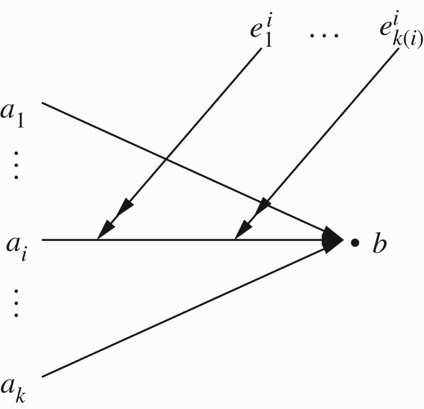
Consider the situation in Figure 11.

Assume a Boolean condition of the form

a=iniff⋁i=1k⋀j=1nεi,j,(∗)

where εi,j can be either x_j= in (can also be written as +x_j) or x_j= out (can also be written as −x_j).

Consider the Boolean function ha corresponding to the Boolean condition (*), as presented in Example 1.13.

ha(f(x1),…,f(xn))=1−∏i=1k1−∏j=1ne(εi,j),

where

e(εi,j)=f(xj)ifεi,jis “xj=in”,1−f(xj)ifεi,jis “xj=out”.

We now implement Figure 11 as a critical subset of Figure 12.

We distinguish three cases:

Case 1: some nodes x do attack the node a, as shown in Figure 11.

Case 2: a is not attacked at all and ha=1.

Case 3: a is not attacked at all but ha=0.

We now treat each case

Case 1: We have new points as follows

(1) Points ua,z1a,…,zka, as in Figure 12.
(2) For every εi,r which says x_r= on, we add a new point yi,ra for i=1, …, k and j=1, …, n. The points {a,ua,z1a,…,zka,yi,ra} are connected as in Figure 12.

the other points in Figure 12 are x1,…,xn.

The point x_r is connected to y_{i, r} if εi,r is x_r= in, for i=1, …, k and r=1, …, n. The point x_s is connected directly to zia if εi,s says x_s= out. (Note that in this case yi,sa does not exist in Figure 12.)

This is done for i=1, …, k and s=1, …, n.

Let us now calculate f(a) in terms of f(x1),…,f(xn).

We get

f(yi,ra)=1−f(xr),f(zi)=π(1−f(yi,ra))·π(1−f(xs)),=πf(xr)·π(1−f(xs)),εi,r=“xris in”εi,s=“xsis out”,=∏j=1ne(εi,j).

We also have

f(ua)=∏i=1k(1−f(zia))

and

f(a)=1−f(ua).

So in total we get

f(a)=1−f(ua),1−∏i=1k(1−f(zia)),1−∏i=1k1−∏j=1ne(εi,j).

As you can see the old points do not depend on the new points.

Case 2. In this case do nothing. The graph for node a is node a as it is.

Case 3. In this case, we want a graph that will give a value 0. So we take a two point graph, with the points a and the point u_a, with point u_a attacking a.

So to summarise, Figure 12 can be either of three figures according to which case occurs for the node a.

Construction 2.12

We now show how to embed a general equational Boolean net (S,RA,f,ha),a∈S in an ordinary Dung network (T,ρ),T⊃S such that the S is a critical subset of T.

Let a∈S and let x1,…,xn be all the attackers of a. We are now in the situation of Figure 11, in either Case 1 or Case 2 or Case 3. Index this figure by a and let (Ta,ρa) be the network associated with the corresponding Figure 12. Note that all new points ua,zia,yi,ra are already indexed by a.

Note also that u_a is a unique attacker of a (Cases 1 and 3) and appears only in (Ta,ρa). In any other (Tb,ρb) in which a may appear, then a attacks a yi,rb or a zib but is never attacked by any of the T_b new points.

Let T=⋃a∈STa and ρ=⋃a∈Sρa.

Then, (T, ρ) is the required Dung networks. Note that for each a we are adding at most n³ points.

Example 2.13

Let us do a simple example, see Figure 13

The conditions are:

aifb,bif¬b.

We can understand a if b as a sort of support, but it does not matter, it is a Boolean condition. We translate the figure into Figure 14.

We have

(1) f(zb)=1−f(b).
(2) f(ub)=1−f(zb).
(3) f(b)=1−f(ub).
(4) f(ya)=1−f(b).
(5) f(za)=1−f(ya).
(6) f(ua)=1−f(za).
(7) f(a)=1−f(ua).

From (1) and (2), we get

(8) f(b)=1−f(ub) which together with 3 give f(b)=12.

Following (4)–(7) gives

(9) f(a)=12.

Notice that y_a, z_a, u_a are just “transmitters” of values from b to a.

Remark 2.14

Remark 2.14Equations for logic programmes

Note that what we called Boolean nets in Example 2.11, where we give up the Dung convention and regard the network as just a general directed graph, are actually logic programmes.

A propositional logic programme contains clauses of the form

aif⋀ibi∧⋀j¬cj.

Note that we may have a clause of the form

in which case we write

aif⊤.

For a fixed literal a, there may be several such clauses with a as the head. We can therefore write them all together as a disjunction of the form

xr=⋁i⋀jxr,i,jεr,i,j,(∗∗)

where x_r ranges over all heads, i ranges over all clauses with heads x_r and x_{r, i, j} ranges over all literals in the ith clause for x_r.

We also have εr,i,j∈{0,1} and the convention that

xr,i,j1=xr,i,j

and

xr,i,j0=¬xr,i,j.

Compare the above with equation (*) of Example 2.11.

Following the discussion in Example 2.11, the equations we get for the logic programme (**) are the following

(♯1) f(xr)=1−∏i(1−∏jfεr,i,j(xr,i,j)),

where f1(y)=f(y) and f0(y)=(1−f(y)) for any y.

The equations are with the variables {xr,xr,i,u}.

(♯2) If x_r is a head of a clause without a body then f(xr)=1.
(♯3) If x_{r, i, j} is not a head of a clause then f(xr,i,j)=0.

Remark 2.15

Remark 2.15Embedding logic programmes into argumentation networks

We wrote in Remark 2.14 Equations (♯1)–(♯3) directly for the logic programme and did not say how to translate the logic programme as a critical subset of some argumentation network. This translation we do now: we need first to transform the original logic programme above to a new equivalent logic programme in which every literal is a head of a clause.

We do this as follows:

There may be literals x in the old logic programme which appear in body of clauses but are themselves not heads of any clause. In this case, we provide a clause for x of the form

xif¬⊤

our understanding that ⊤ is a literal which always succeeds (gets value 1). So the literal x always fails.

Thus, we get a new programme with one more literal, ⊤, and some additional clauses, and this new programme is equivalent to the original, and in this programme every literal (except ⊤) has a Boolean equation like (**) associated with it.

Now we construct a Boolean network (S, R_A) as follows:

(1) The set S of nodes are all the literals of the new logic programme.
(2) Let x_r be any literal in S different from ⊤. Assume x_r is connected in the new logic programme via (**) to the literals x_{r, i, j}. Then, let xr,i,jRAxr hold.
(3) Let the Boolean equation for x_r be (**).

We now have a Boolean network and we use Construction 2.12 to embed it as a critical subset of a Dung network.

The overall result is the embedding of the original logic programme as a critical subset of a Dung network.

Remark 2.16

We noted in Gabbay and d'Avila Garcez (2009) that ordinary Dung networks can be translated to logic programmes in a very direct manner. If x1,…,xm are all the nodes attacking x then we write the clause

xif⋀i¬xi.

In Wu, Caminada, and Gabbay (2009), we discuss in detail the connection between argumentation networks and logic programmes.

The equational approach allows us to give fuzzy values to logic programmes. The much discussed loop problem resolves itself automatically. Consider Example 1.10. Figure 9 considered as a logic programme yields

cif¬b,aif¬c∧¬a,bif¬a∧¬b.

We got fuzzy values as solutions.

It is worthwhile to investigate an equational approach to fuzzy logic programming.

Remark 2.17

Remark 2.17Discussion of Brewka and Woltran 2010

Note that Brewka and Woltran (2010) introduce and study what they call abstract dialectical framework (what we call Boolean nets or logic programmes). They need to define extensions for their networks. We got Boolean functions either as a side effect of fibring in Gabbay (2009b) or as a natural equational example in the current paper. We find our extensions by solving equations or by critically translating into ordinary Dung networks. Brewka and Woltran need to do something similar. Their options are as follows:

(1) Define the new notions of extensions for their networks and provide algorithms as Dung did for framework; or
(2) Use the present paper with Brouwer's fixed point theorem and use MATLAB or MAPLE or NSolve to find the solution; these solutions might be more refined than the extensions they would get in Brewka and Woltran (2010), as we have seen in Remark 1.6; or
(3) Another option is contained in Gabbay (2009b) on fibring argumentation networks. In this paper, I studied what happens when we substitute one Dung network inside another. In the course of this study, I got networks with Boolean conditions of the form
- • a is out if ⋀ixi= in
and the form
- • ⋁ixi= out if a= in
and to find the extensions of such networks I translated in detail with examples the Boolean conditions into ordinary Dung networks and defined the notion of critical subsets, etc.

These notions are used in Example 2.11 of this paper.

Note that for equational networks, we do not need the translation and the additional nodes. They disappear from the final equation, as we saw in the calculations of Example 2.11.

Remark 2.18

The reader is advised to consult our paper (Gabbay), especially Section 2.4.entitled: Why are we not surprised by results of Gabbay, Brewka, and Woltran?

The paper shows the equivalence between Dung's argumentation networks and classical logic with the Peirce–Quine dagger connective, and therefore Dung's argumentation is as expressive as classical logic, Dung's networks can represent any Boolean network or logic programme, as shown in Gabbay.

Remark 2.19

Remark 2.19Finding extensions

The question of how to use the equations for finding extensions will be discussed in a later section.

We can always find all solutions to the equations and this will give us all the extensions and then use extra secondary examination to classify them. However, this is not what we mean.

We want to modify the equations to give us the desired extensions as solutions.

We can do this now for finding stable extensions as follows.

The stable extensions give either 0 or 1 values to all nodes. This means that the new variable y defined below must solve to value 0:

y=∑x[f(x)·(1−f(x))].

So we add a variable y with equation as above and tell the math program such as MAPLE or MATLAB or NSolve to output solutions for y=0, if possible.

Summary Remark 2.20 (Advantages of the equational approach)

We now list the advantages of our approach:

First let us highlight the fact that given a traditional argumentation network with attacks only, we regard it as a graphical generator of equations, and we use equations as a conceptual framework. We no longer talk about concepts such as defense, acceptability, admissible extensions, etc. but talk instead about solutions to the equations.

Therefore, conceptually, we have

• an extension is a solution to the equations and different extensions (grounded, preferred, stable, semi-stable, etc.) are characterised by further constraints/equations on these solutions functions using say Lagrange Multipliers, see Section 6 below.

Within this framework, we note the following:

(1) To find all possible extensions, we solve equations. We feed the equations into existing well-known mathematical programs such as MAPLE or MATLAB or NSolve and get the solutions. See also Remark 2.19.
There are many papers which calculated computational complexity of finding various extensions, when we reduce the problem to that of solving equations in MAPLE or MATLAB or NSolve, complexity is not reduced, it can only increase.
What do we gain then?
- • A new uniform framework, not only for argumentation networks, but also for other types, ecological, flow, etc.
- • Possibility of finding different heuristics for equations which will work faster for most cases, giving an advantage over non-equational algorithms.
- • Ordinary people such as lawyers, etc.; to the extent that they use argumentation at all and are not averse to formal logic, they may find that it is psychologically easier to plug the problem into the computer, go and make a cup of tea and then check the results.
Furthermore, if we insist on certain arguments being in or out, we can experimentally feed this into the equations and test the effect on other arguments. MATLAB itself does not generate all the solutions automatically but requires initial input, which is an advantage if we have a special set of arguments in mind.
For example, the question of whether a set of arguments belongs to some extension (being credulous) of a certain type or whether the set belongs to all extensions of a certain type (being sceptical) can very naturally be handled in the equational framework.
To generate all extensions, we need to keep plugging initial conditions into MATLAB; that is, plug in all possible candidates for extensions (this is exponential in the number of nodes but we saw in Remark 2.15 and Construction 2.12 that any Boolean set of functions can be embedded in argumentation networks, and so the complexity is exponential anyway).
Another possibility is to use NSolve which does generate solutions, see http://reference.wolfram.com/mathematica/ref/NSolve.html.
Another disadvantage of this is that we might get approximate solutions. So if we get x=0.999, we ask is this for real or is the solution supposed to be x=1?
On the other hand, an advantage of using such programmes is that it makes it easy to incorporate argumentations feature into other larger AI programmes, as almost anything allows for solving equations.
(2) We have a framework for introducing support as we shall see in the next section.
(3) Note the word of caution and comments in Section 3.1.

3.Analysis of support

The purpose of this section is to develop equations for networks of the form (S, R_A, R_S), where R_A is the attack relation and R_S is the support relation. Figure 2 is an example of such a system, but in this section we will have proper equational theory and many examples.

3.1.Caution about support

We begin with a word of caution. Our equational model for attack ends up with numbers between 0 and 1 labelling the nodes of the graph (S, R_A) with x=1 meaning “x is in” and x=0 meaning “x is out”. The value f(a)=ha(f(x1),…,f(xn)) gives the impression that x₁ is to be considered as attacking a if by increasing f(x1) we decrease f(a) and therefore we are tempted to say that x₂ supports a if by increasing f(x2) we are increasing the value of f(a). This view is encouraged by situations as in Figure 15.

The equations are:

(1) f(a)=(1−f(x1))(1−f(x2)).
(2) f(x2)=1−f(y).
(3) f(x1)= some function of its further nodes.
(4) f(y)= some function of its further nodes.

We therefore see that

f(a)=(1−f(x1))·f(y).

So y is supportive, because if f(y) increases then f(a) increases. We can also see this immediately from Figure 15 because y attacks x₂ which itself attacks a.

So the idea we might consider is that of the clear support of any node y of a node a can be read from the functional equations. The reading may not be immediate, as can be seen from Figure 16, but we are able to define what support is!

In Figure 16, the equations are:

(1) f(a)=(1−f(x))(1−f(u)).
(2) f(x)=(1−f(y))(1−f(u)).
(3) f(y)=1−f(u).

Hence,

f(a)=(1−f(u))(1−f(u)(1−f(u))).

Whether f(a) is increasing in [0, 1] when f(u) is increasing needs to be checked by tracing the curve.

Our cautionary comment is that this is the wrong approach!

The numbers we get for the nodes as the result of the equation have no qualitative meaning beyond the fact that they indicate which points are in, out, or undecided. They do not indicate strength of argument and therefore cannot be used to indicate support.

To make this point crystal clear, consider again Figure 9. We got solutions for this figure, namely:

f(a)=1−22,f(b)=2−1,f(c)=2−(2).

These numbers say that the nodes a, b, c are all undecided and may indicate the types of loops we have in the original graph (though we have not developed such a theory yet, this is postponed to a subsequent paper. See, however, Gabbay (2012a,b), where we discuss the methodology of loops). They are not indicating strength of arguments!

Figure 7.

Double loop.

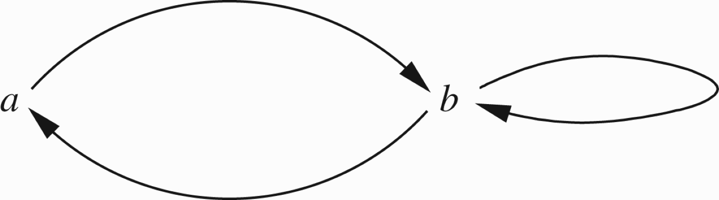
Figure 8.

Symmetrical double loop.

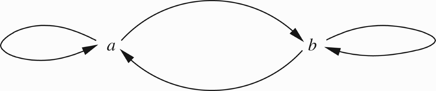
Figure 9.

Asymmetric loop.

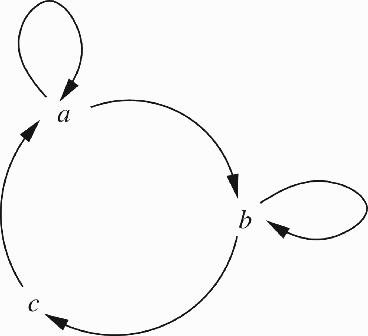
Figure 10.

A loop for example 1.11.

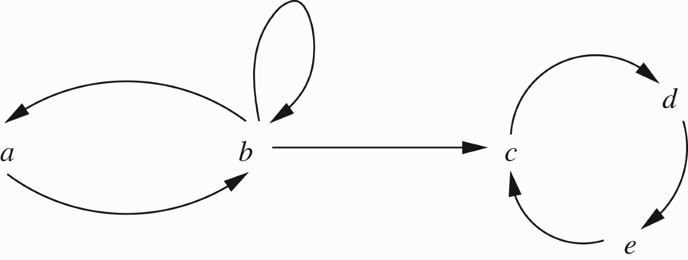
Figure 11.

A general attack situation.

Figure 12.

A figure containing Figure 11.

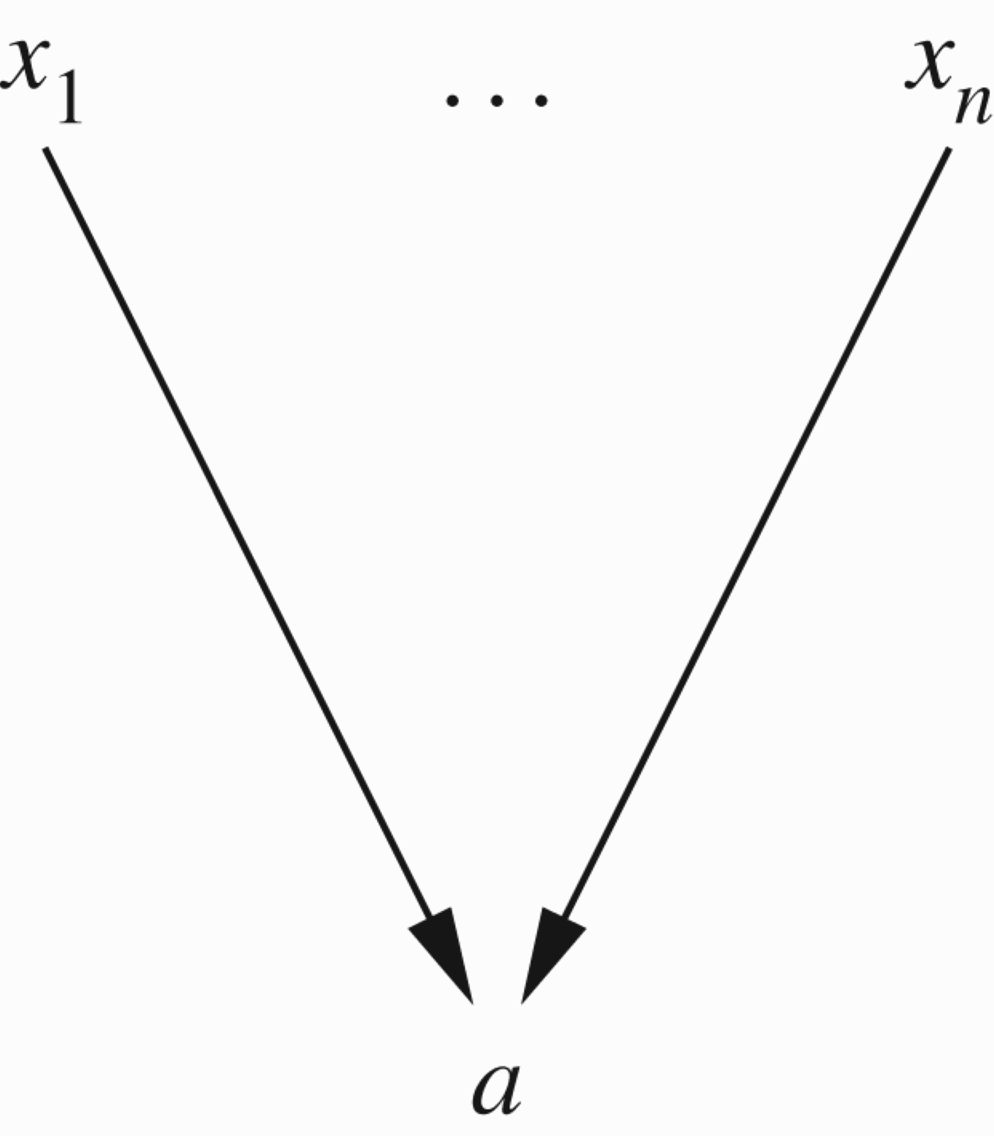
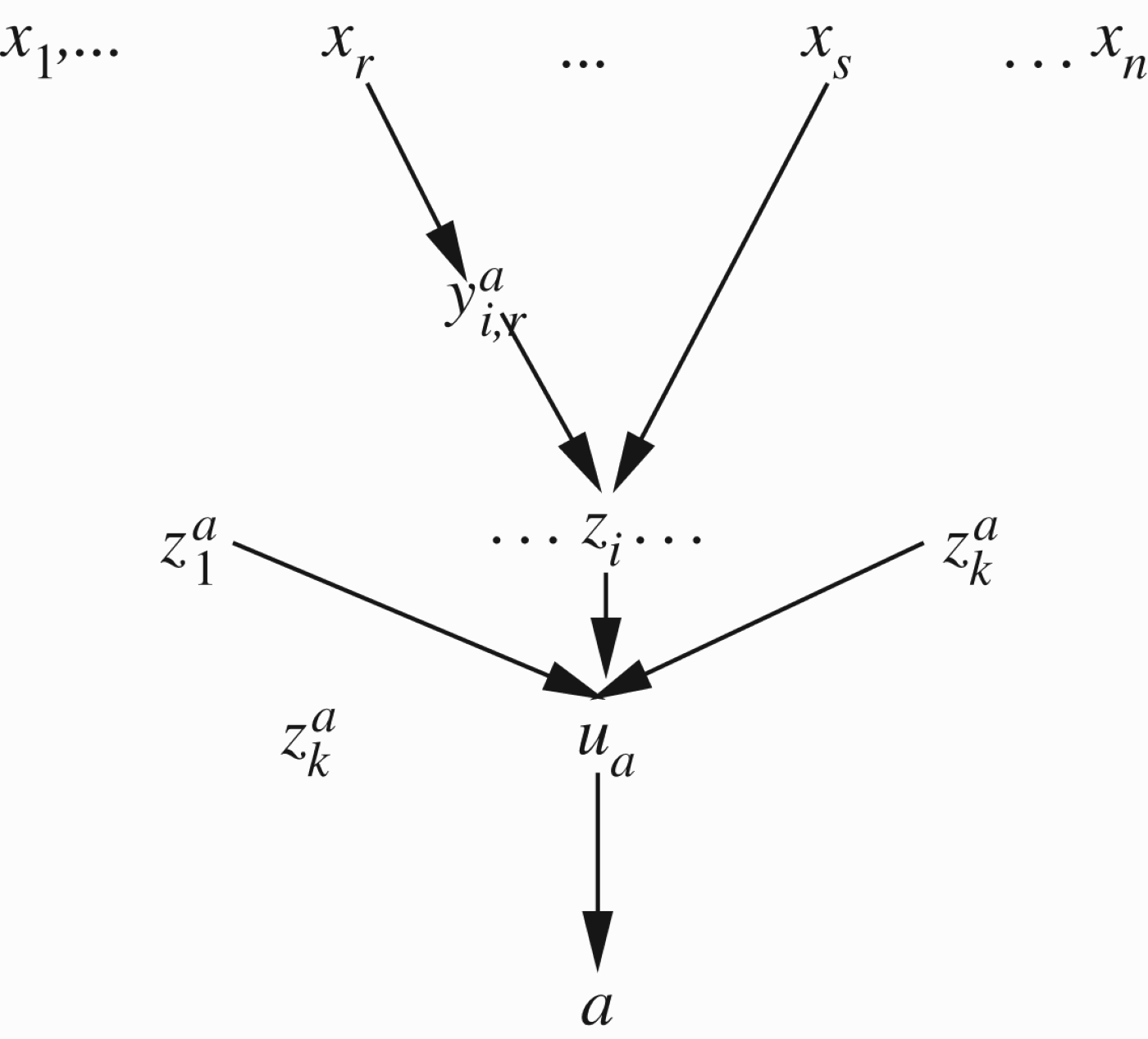
Figure 13.

Illustrating Example 2.13.

For comparison, let us view Figure 9 as arising from some ecology on an island. a, b and c are species which prey on one another.

a can eat b but can also cannibalise themselves. b can eat c and also b and c can eat only a. Of course, there should be some ecological balance where the number 0⩽f(x)⩽1 tells us the stable percents of population x which exists under equilibrium.

The equation

f(x)=ha(f(x1),…,f(xn))

tells us the size of species a facing its predators (attackers) x1,…,xn as a function of their size f(xi). Thus, the solutions f(a)=1−22, f(b)=2−1, and f(c)=2−2 represent a stable ecology.

One can see immediately that the set of equations Eq_max is not suitable for the ecological model. Predators combine their effect, not politely allow the strongest to do the job. Eqinverse is more suitable and from these equations, we get the above solution.

These kinds of ecological and other flow networks were studied extensively in Barringer et al. (2005) and contained the equational argumentation networks as a limiting case. In this context, we can indeed say that y supports x if an increase in f(y) generates an increase in f(x).

We recommend that the reader should look at our papers Barringer et al. (2005) and Barringer, Gabbay, and Woods (2012) and also Barringer et al. (2008), we believe that they are of value to the argumentation community.3 3

3.2.Equational model of support

We saw in Section 3.1 that we need a conceptual motivation for support rather than use the equations produced by the attack. So let us offer a model and compare its results with the literature. Our starting point is a network of the form (S, R_A, R_S), where S is a set of arguments, RA⊆S2 is the attack relation and RS⊆S2 is the support relation. We need to decide what kind of equations ha to offer for such a network. Our considerations must be qualitative in the context of argumentation (as opposed to, for example, ecology, fluid flow, etc.). Before we start, we need a word of caution. Support is not a simple concept and, in argumentation, many serious authors have tried to address it. In this serious context, the reader should not expect much from the numerical equational approach. When we use numbers, we are forced to simplify. We academics know very well that when we apply for a promotion, our performance is reduced to impact factors and number of papers and other numbers, which in many cases does not reflect our real contributions. So, the most we can expect from the numerical equational approach is common sense reasonable soundness. In our numerical paper (Barringer et al. 2012), for example, we even considered the possibility of an assumption that attack and support by the same strength should cancel each other out. This makes sense as a soundness condition on the numerical functions.

Let us start with the simplest of diagrams, Figure 17

Figure 14.

Translating Figure 13.

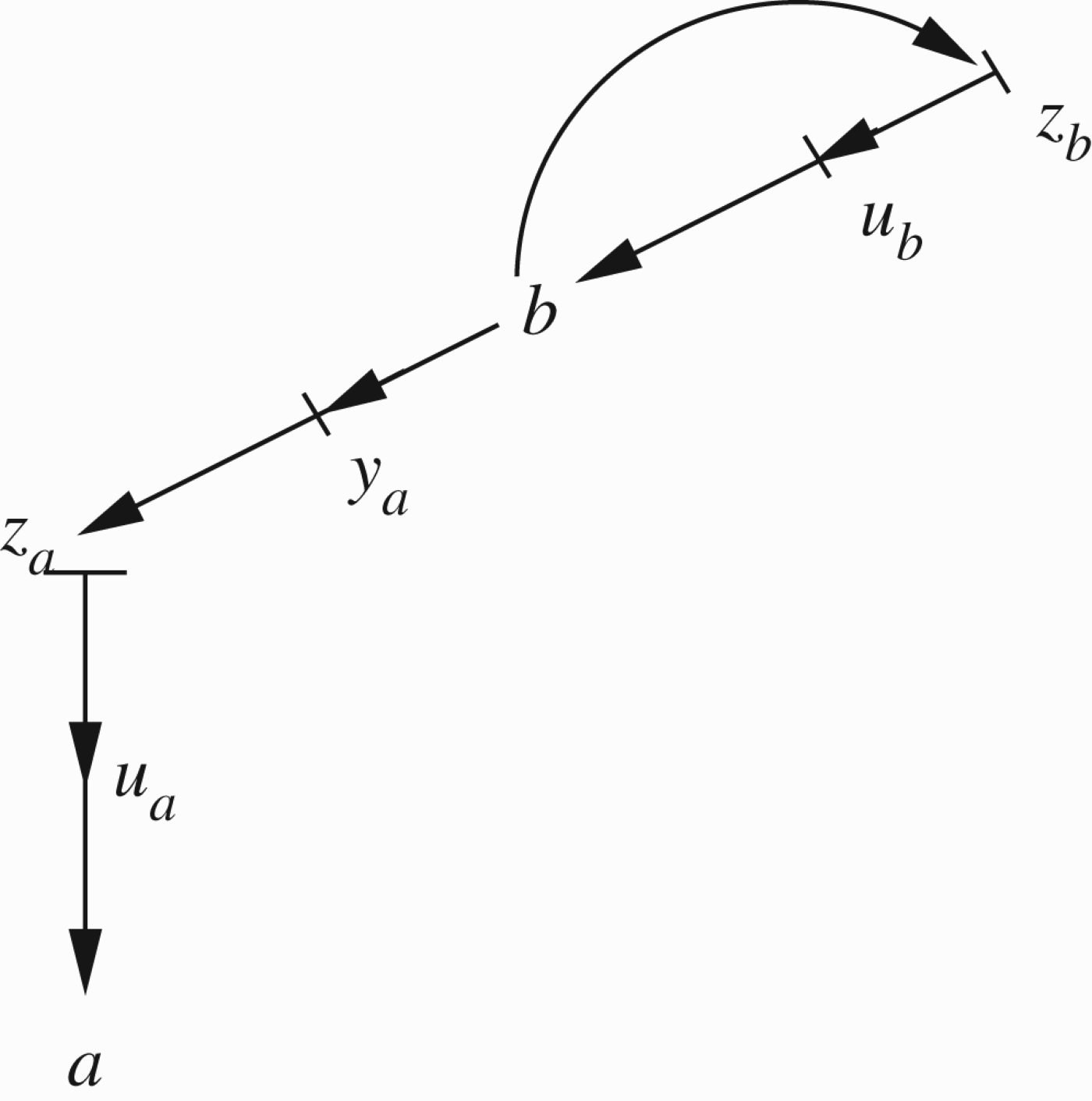
Figure 15.

Caution about support.

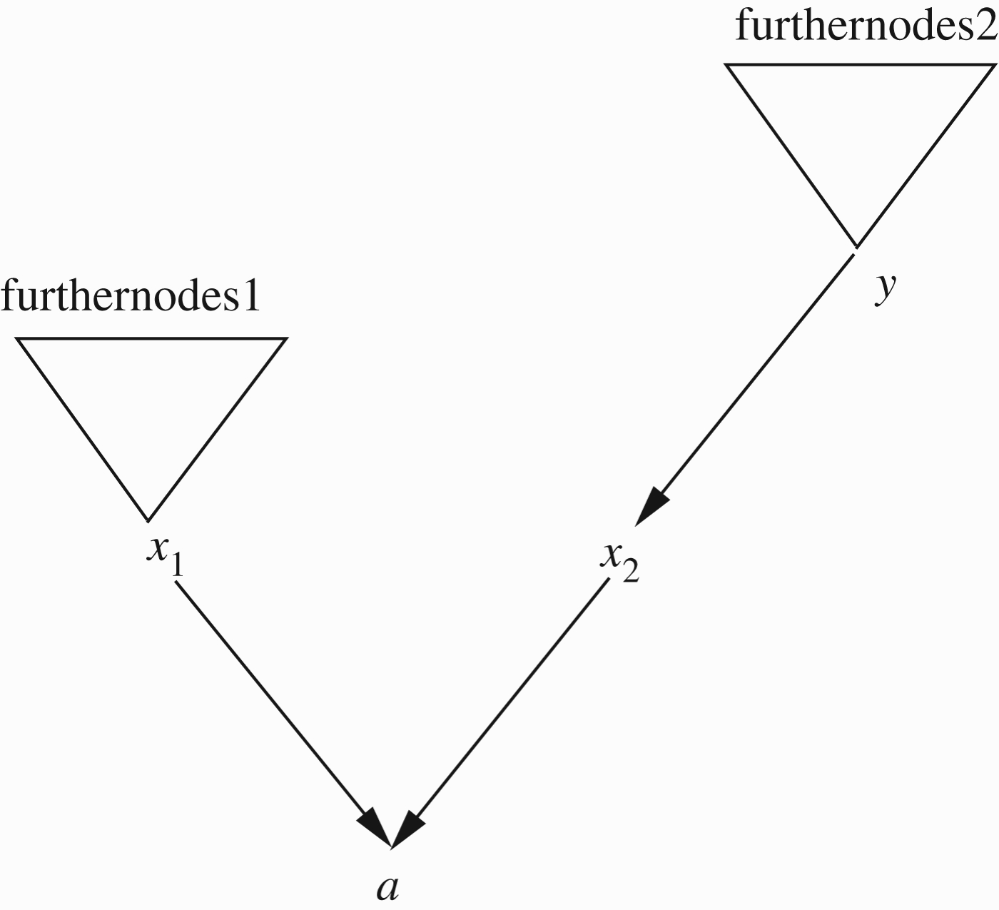
Figure 16.

Illustrating Equational support.

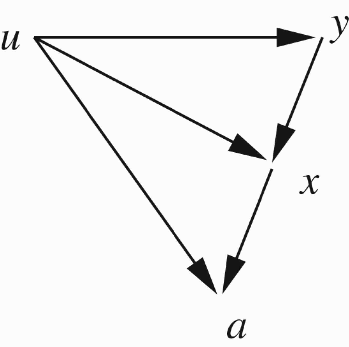
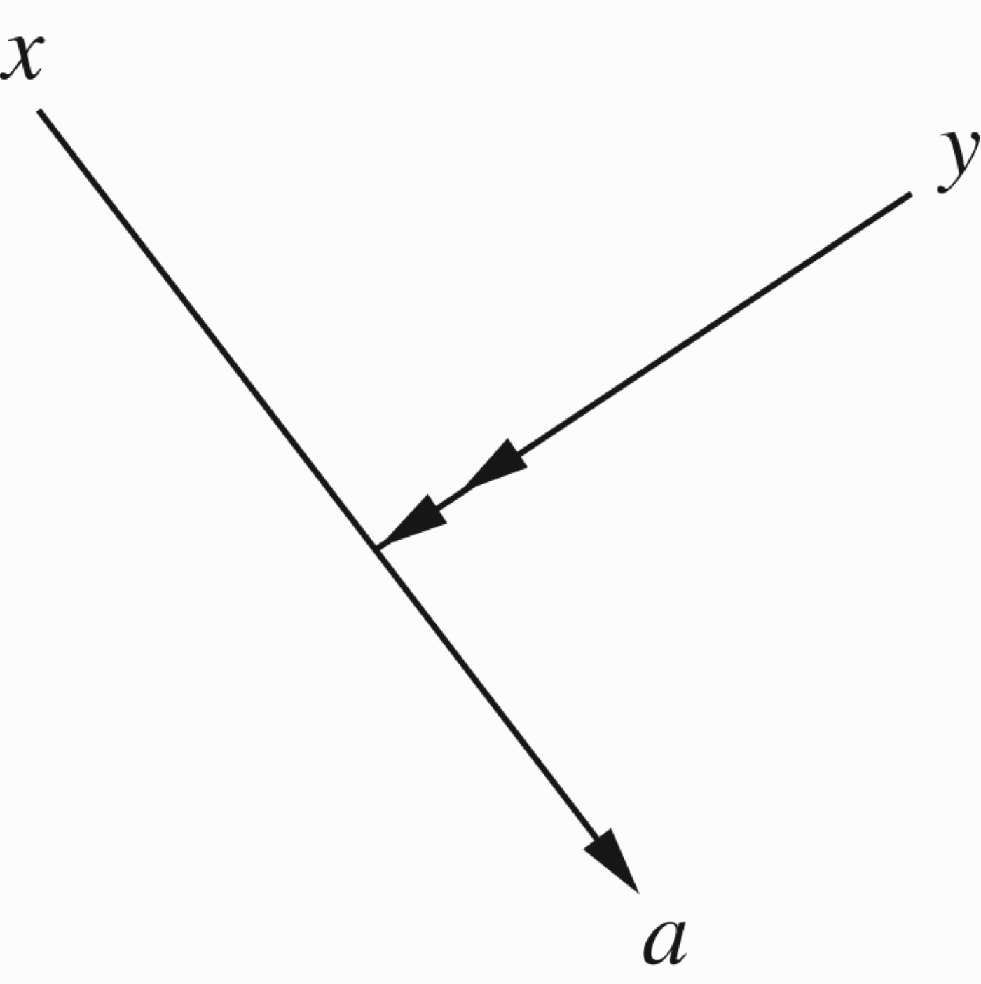
Figure 17.

Attack and support.

The argument a is attacked by x and is supported by y.

S={a,x,y}.RA={(x,a)}.RS={(y,a)}.

The question is: should a be in or out, or more generally, what value to give a as a function of the values of x and y. This of course depends on the intended meaning of support, but is restricted by the parameters available to us in the numerical context. We cannot capture much meaning with numerical functions.

This is discussed extensively in Barringer et al. (2005, Section 4.1) with a view (Barringer et al. 2005) that equations should be sought which allow x and y to cancel each other if they have the same strength.

We shall not go into this in this paper. See, however, Remark 4.9 in Section 4.

Our graph networks have no strength and so there is nothing we can say about Figure 17. We can adopt a risk-averse approach and say if a is attacked by anything then a is out. This is certainly the attitude of government funding bodies; one negative review and your application is out! So the risk-averse approach will allow for the extension a= out, x=y= in.

Let us offer a definition. We adopt a risk-averse approach!

Definition 3.1

Definition 3.1Threats

Let (S, R_A, R_S) be an argumentation network with attack and support. Define two auxiliary relations for the purpose of defining equations. The definition will be schematic, dependent on a parameter relation R, which will allow us to perform iterations. Let R⊆S2 be any relation defined already using R_Aand R_S. We define ρ₁(R) and ρ₂(R).

Option 1

uρ1(R)xiff def.uRx∨[∃z∃n(xRSnz∨uRz)].

Option 2

uρ2(R)xiff def.uRx∨[(∃z∃n(zRSnx∧uRz)].

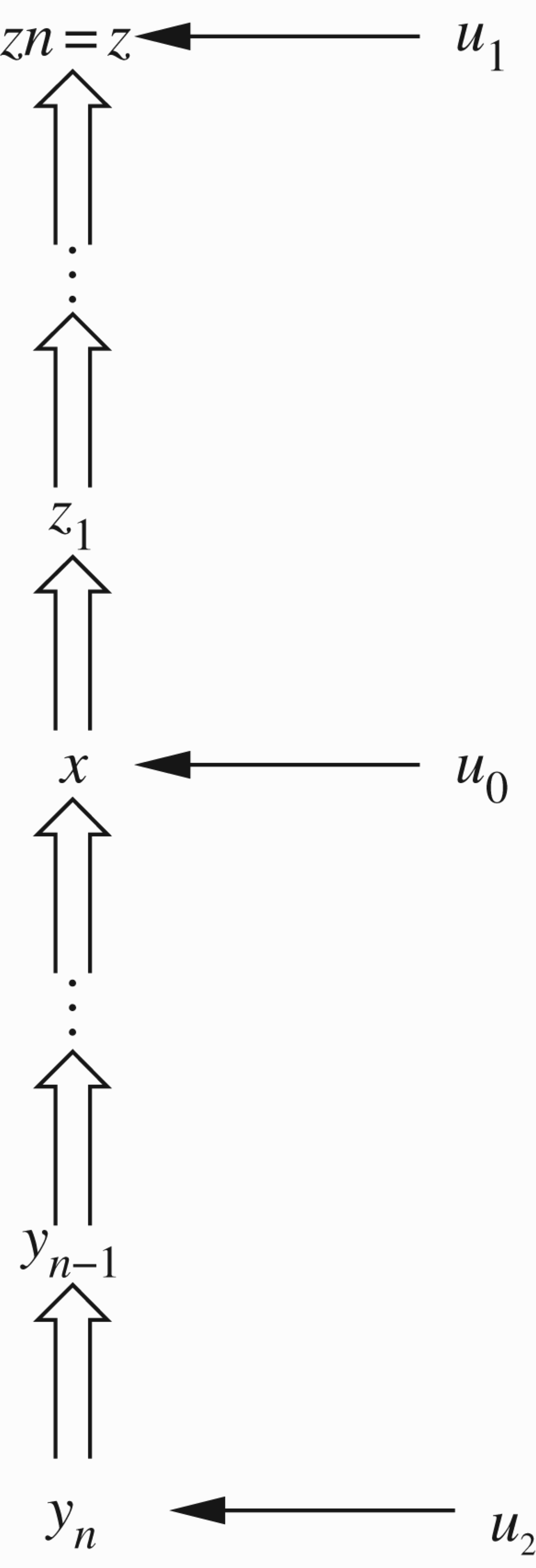
The meaning of uρi(RA)x is that x is under threat from u.

Figure 18 explains the situation.

In Figure 18, node u₀ attacks x directly, it is therefore both ρ₁(R_A) and ρ₂(R_A) threat to x.

u₁ attacks z which is at the end of a chain of support from x. According to ρ₁(R_A), u₁ is a threat to x. It undermines x’s credibility.

u₂ attacks a great grandparent supporter of x. Again it can be a threat to x.

The process can be iterated. We can look at ρ1(ρ1) and ρ2(ρ1),ρ1(ρ2),ρ2(ρ2). See Example 3.3.

Let ρe→ be an arbitrary ρe1(ρe2(…ρen(RA)…)), where e→=(e1,…,en) and each ei∈{1,2}. So ρe→ is an arbitrary iteration of ρ₁, ρ₂.

We can use ρe→ to define the equations for the network. This means that we use n-level threats to define our equations. So, the role of support in the network is to propagate different levels of threats on a node x through the networks by means of direct R_A attacks on various supporters or supported nodes related to x.

A policy of handling support will choose ρe→ or a combination and define the equations accordingly, as in Definition 3.2. See also Remark 4.9.

Figure 18.

More elaborate attack and support.

Definition 3.2

Definition 3.2Equations for support

Let (S, R_A, R_S) be a support network and let ρ=ρe→ be as in Definition 3.1. Define Eqρ(f) to be

f(a)=∏i=1n(1−f(ui)),

where

{u1,…,um}={u|uρe→a}.

So for the case of ρ_i(R_A), there are two definitions. One for each ρ_i(R_A).

We understand the empty product to yield 1 (i.e. f(a)=1 if ¬∃uuρa).

Note that our later discussions of higher level attacks in Section 4 below also suggest further equations for support. See Remarks 4.9 and 4.10.

We now examine examples from the literature. We use ρ.

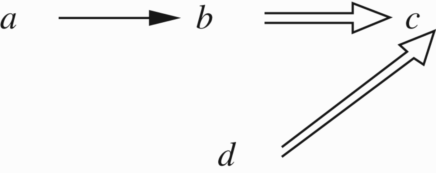
Example 3.3

Example 3.3Figure 4 from Boella et al. 2011b

Consider Figure 19.

We have that aρ2(RA)c and aρ1(ρ2)(RA))d, but a is not a ρ₁(R_A) threat to c. So depending on how far we want to look for threats, our extensions can be either {a,d,c} if we look at ρ₁(R_A) only, or {a} if we look at all of ρ1(ρ2(RA)), or we can look at both ρ₁(R_A) and ρ₂(R_A).

We have no need to explicitly write the equations here, as the results are clear.

For comparison with the literature, note that according to Boella et al. (2011b, 2010) (which does not use equations but meta-level variables), we do get {a,d,c}. Cayrol and Lagasquie-Schiex (2005, 2010) get {a}, while Oren et al. (2010) also get {a,d,c}.

We shall comment that the equational approach is very simple, while Cayrol and Lagasquie-Schiex (2005, 2010) and Oren et al. (2010) are very involved. See Remark 2.20.

It is still open to characterise other approaches such as Cayrol, Oren, or Brewka in terms of equations.

Figure 19.

Support down the line of attack.

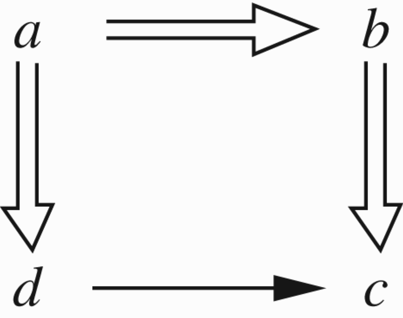
Example 3.4

Example 3.4Figure 14 from Boella et al. 2011b

Consider Figure 20

In Figure 20, node d ρ₁(R_A) attacks node a. Node d also ρ₁(R_A) attacks nodes b and c. Thus, the only extension according to ρ₁(R_A) equations is {d}. Both Cayrol and Lagasquie-Schiex (2005, 2010) and Oren et al. (2010) get {a,d}. See Boella et al. (2011b, 2010) for a discussion.

Figure 20.

Support up the line of attack.

Example 3.5

Example 3.5Gabbay–Villata comparing example

Consider the following example for the purpose of comparison, see Figure 21.

These are the fighting parents, a and b example, who each support their child c.

a ρ₂(R_A) attacks b and c.

b ρ₂(R_A) attacks a and c.

However, if we do not use ρ₂, then ρ₁ does not affect c.

(1) According to ρ₁(R_A), equations in the extensions are
- (a) a=1, b=0, c=1.
- (b) a=0, b=1, c=1.
- (c) a=½, b=½, c=1.
(2) According to Boella et al. (2011b), c is always in and {a,b} from a two elements loop.
(3) According to Oren et al., we have arguments as sets, so we have two possibilities. See Figures 22 and 23. Note that Oren et al. (2010) always adds an almighty source of support 𝒩.
(4) Cayrol and Lagasquie-Schiex (2005, 2010) get essentially the same as Oren.

Figure 21.

Floating support.

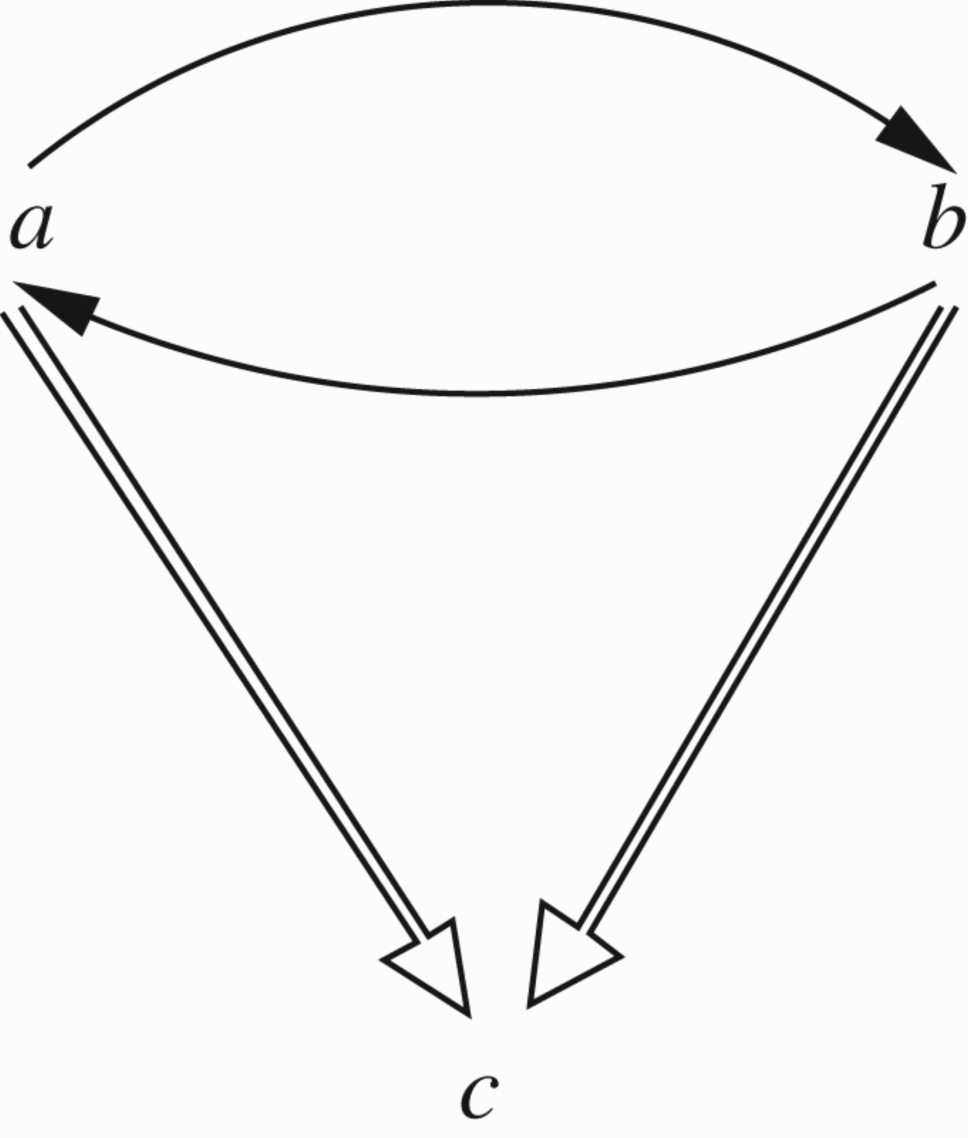
Figure 22.

Aggregating support and looping.

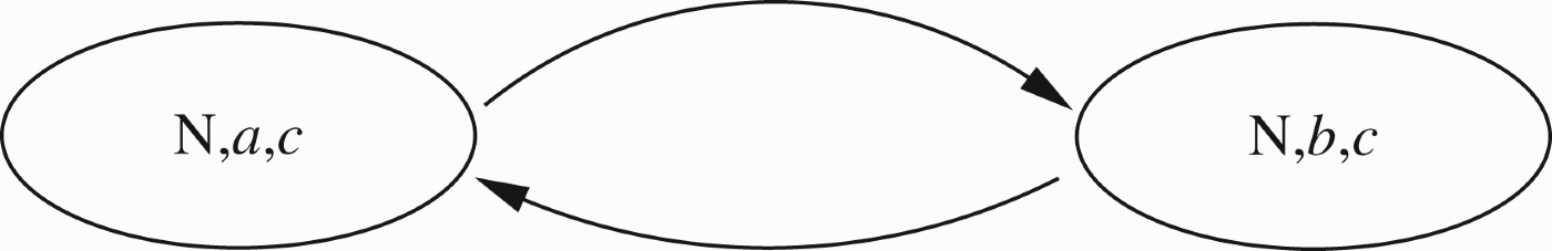
Figure 23.

Aggregating support and self looping.

Example 3.6

Example 3.6Brewka and Woltran 2010

Brewka and Woltran example in Figure 24 is an interesting key example. It is also discussed in Boella et al. (2011b) as Figures 5 and 18 of Boella et al. (2011b).

Here it is:

Brewka and Woltran put this forward as a counter example to Cayrol, who supports the extension {w,s}. If we adopt ρ₁(R_A) equation, we get {w,c,s}. If we adopt ρ₂(R_A) equation, then w is a threat to c, as well as to r. So we get {w,c,s}.

Brewka and Woltran give a specific meaning to this example and argue that the attack of w on r is stronger than the support of c to r. As we discussed in Section 3.1, when we add strength to our networks we are playing a different game. In Boella et al. (2011b), we interpret Brewka and Woltran's argument as a higher order attack as in Figure 25.

The double arrow attacks the support arrows.

This type of double arrow was extensively used in Barringer et al. (2005) and Gabbay (2009c) and was also independently used by Modgil (2009) and treated by Baroni, Cerutti, Giacomin, and Guida (2009).

It is what I call a reactive arrow, originally introduced by Gabbay in 2004, see Gabbay (2008) and widely applied in many areas, such as deontic logic, automata theory, multi-agent systems, formal grammars, and so forth.

It is a different game altogether and we shall analyse its equational semantics in a later section.

Figure 24.

Support to the middle of the attack line.

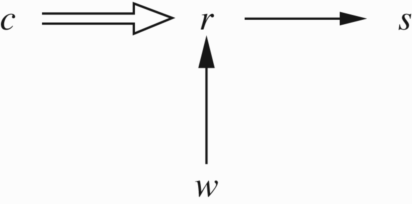
Figure 25.

The need for higher level attacks.

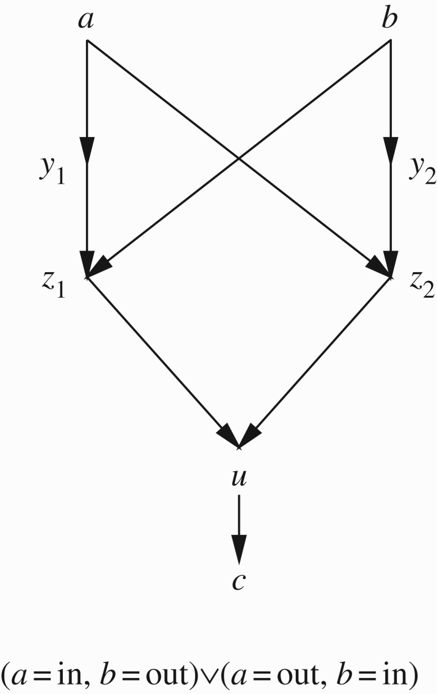
Example 3.7

Example 3.7Brewka and Woltran 2010

In their paper, Brewka and Woltran (2010) gave the following Boolean example, see Figure 26. The connection with support is that the condition on c is that c= in provided that the values of a and b are different. So if b= out then the arrow a→c is support and if b= in then the arrow a→c is attack. Following Example 2.11, Figure 26 can be represented as the ordinary Dung network of Figure 27.

Figure 26.

Boolean dependence.

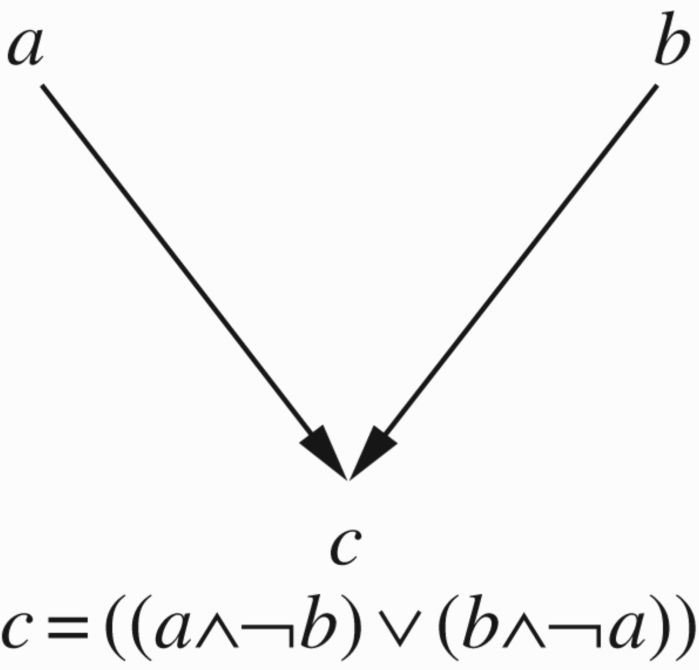
Figure 27.

Implementing Boolean dependence.

4.Equations for higher level attacks

The case of higher level attacks is the strong evidence for the success of the equational approach. The historical story runs as follows.

In Barringer et al. (2005), we introduced networks with higher level attacks of any kind. Figure 28 is a typical situation.

Figure 28.

Higher level attacks on attacks.

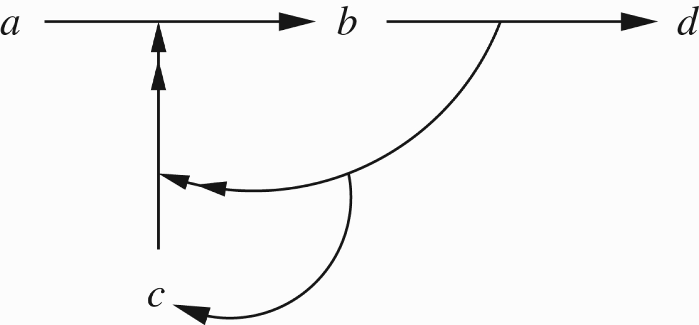
Figure 28 can represent any kind of network, not necessarily an argumentation network. It can be part of a Kripke model, an electrical network, a biological ecological network, etc. In each case, the arrows have their own meaning. The paper by Barringer et al. (2005) also allowed for value annotations to the nodes and arrows and gave algorithms for the propagation of these values.

In the case of argumentation networks, the nodes are arguments and the arrows mean attacks. The values (annotations) can correspond to the equational labellings and the propagation of values are governed by the properties of the equations.

The aim of this section is to interpret (give equational semantics) to higher level attacks, in the case of argumentation networks.

Let us look again at Figure 28, reading it as an argumentation frame.

In Figure 28, the argument c attacks the attack from a to b (we use the notation c↠(a→b)), while the attack from b to d attacks the attack emanating from c (notation (b→d)↠(c↠(a→b)). This later attack attacks c (notation ((b→d)↠(c→(a→b)))↠c).

The question we ask is how to define the possible acceptable extensions for {a,b,c,d} for the network of Figure 28. The reader should note that whatever approach we give for defining extensions, it must come from reasonable general principles which are meaningful for general networks. It should not rely on very specific features of argumentation networks. The general principles can have a specialised meaning in the argumentation case, but then equally the principles can have their own meanings in the case of other networks. We shall use equational principles.

Modgil (2007) independently defined a higher level attack networks where arrows emanating from nodes can attack other arrows (like c↠(a→b) in Figure 28). Modgil defined certain restrictions on his networks and tried to define a suitable notion of extension in the traditional setting of admissible sets. His paper was studied by Hanh, Dung, and Thang (2010) on account that his definition of extensions was not monotonic. Hanh et al. supplied their own discussion and definitions. The disagreement focussed around the illustrative example of Figure 29. Modgil allowed the extension {c,c1,a}, while Hanh et al. insisted on {c,c1}.

Figure 29.

The Hanh Modgil disputed example.

Meanwhile, two other papers (Baroni et al. 2009; Gabbay 2009c) addressed the semantics of higher level attacks in the Dung style. For a survey and discussion, see Gabbay (2009c).

We shall offer two equational systems for higher level attacks which will settle in two pages the long and tortuous discussions and definitions of the above papers.4 4

Note that since we are writing equations, we are guaranteed the existence of extensions!

To be able to present our case, we need some definitions.

Definition 4.1

Definition 4.1Higher level argumentation frames for attacks emanating from points

(1) An ordinary argumentation frame has the form A=(S,R), where S is the set of arguments and R⊆S×S is the attack relation.
(2) A level (0, 1) argumentation frame has the form A0,1=(S,(R)), where S is the set of arguments and (ℝ) is a set of pairs of the form (x, y) or (z, (x, y)), where x, y, z∈S. (x,y)∈(R) means that x attacks y and (z,(x,y))∈(R) means that z attacks the attack (x, y).
(3) Level (0, n) argumentation frames are defined as follows
- (a) A pair (x,y)∈S×S is called a level (0, 0) attack.
- (b) If z∈S and α is level (0, n) attack then (z,α) is a level (0, n+1) attack.
- (c) A level (0, n) argumentation frame has the form A0,n=(S,(R)), where (ℝ) contains attacks β of level (1, m) for m≤n, including some elements of level (0, n).

To explain our ideas and address Figure 29, let us first define equations for level (0, 1) attacks only. A typical situation is described in Figure 30.

The attackers of b are a1,…,ak and the attacking arrow ai→b is attacked by e1i,…,ek(i)i. Since we restricted ourselves to level (0, 1), there are no attacks on the double arrows eji↠(ai→b).

We now offer the following two options for equations for f(b) (“H” stands for “higher” and “1” stands for “(0, 1) attacks”).

Option H1Eqinverse(f):

f(b)=∏i=1k1−f(ai)·∏j=1k(i)(1−f(eji)).

Option H1Eqmax(f):

f(b)=1−maxif(ai)·1−maxj(f(eji)).

We now see what kind of extensions we get for Figure 29.

Figure 30.

A typical situation for higher level attacks.

Example 4.2

Example 4.2Modgil vs. Hanh et al.

(I) We first use the H1Eqinverse equations for Figure 29. We write x instead of f(x):
- (1) a=1−b.
- (2) c₂=1−c₂.
- (3) c=1.
- (4) c₁=1.
- (5) b=1−c(1−b1).
- (6) b1=(1−c2)(1−c1(1−b)).
  From (2)–(4), we get c=c₁=1. c2=12.
  From (5), we get
- (7) b=b₁
  and from (6), we get
- (8) b1=12b1.
  The only solution is b₁=b=0.
  From (1) we get a=1. Thus, the only extension is a=c=c₁=1, b=b₁=0, c1=12.
  This corresponds to the Modgil extension.
(II) We now use H¹Eq_max. The equations are
- (1) a=1−b.
- (2) c₂=1−c₂.
- (3) c=1.
- (4) c₁=1.
- (5) b1=1−max(c2,c1(1−b)).
- (6) b=1−c(1−b1).
  We get c2=12, c=c₁=1. b=b₁. Thus from (6), we get
- (7) b1=1−max(12,1−b1).
  There are two solutions b1=12 and b₁=0.
  We also get two corresponding solutions for a: a=½ and a=1.
  We thus have the second extension for the case of b1=12 is the Hanh et al. extension c=c₁=1 and b=b1=a=c2=12.

We now address the general case of arbitrarily high level of attacks on attacks. To do this right, we need high level of induction and it can be complicated, as you can see from Figure 31.

This iteration can go on for many levels and we cannot practically handle it for each b and write very long iterated equations. We need an idea, a trick, to go around it. Fortunately, we have it already in Barringer et al. (2005), see Example 2.3 of Barringer et al. (2005) in which we calculate the values for Figure 33 (our Figure 32 is Figure 5 in Barringer et al. 2005). The idea is very natural and very simple.

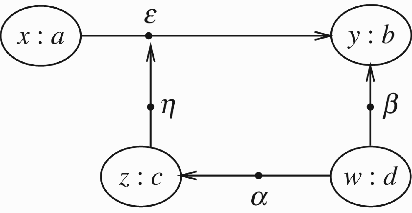
In the paper by Barringer et al. (2005), we have arrows attacking arrows and both arrows and nodes were annotated with numbers. The numbers annotating nodes correspond to strength (when the node is an argument this is the strength of argument) and the numbers annotating arrows indicate strength of transmission. We now quote directly from Barringer et al. (2005), reproducing Figures 4 and 5 of Barringer et al. (2005) as our own Figures 32 and 33 here in this paper, and quote what we wrote about them in Barringer et al. (2005).

Begin quotation from Barringer et al. (2005):

In Figure 33, ϵ is the transmission factor, weakening b in a way that takes account of x: a.

b is also attacked by d with factor β.

However, factor ϵ is attacked by argument c, which is itself attacked by d, with transmission factor α.

This model has two innovations.

(1) The strength of nodes and the transmission factor.
(2) The idea that the transmission factor can itself be attacked.

What kind of network does Figure 32 represent? First, note that the strength of nodes is actually a colouring of them. One might expect us to introduce a transmission factor between colours, then in Figure 32 ϵ could depend only on x and y. We choose to make ϵ depend on the nodes, taking into consideration that the transmission factor depends on the nature of the argument and not just on their strengths. The option of attacking transmission factors enables us to delete attacks, one by one, by attacking (lowering) their transmission factor.

End quotation from Barringer et al. (2005).

So what do we do in our case of Figures 30 and 31, we regard the arrows of any kind for example x↠β as transmission arrows and regard the attack of the form y↠(x↠β) as an attack of y on the transmission factor ε(x,β).

All we need to do now is to give the equation for an attack of the form of Figure 32.

But this situation and the equation for it is very obvious and intuitive. If an argument a of strength x attacks an argument b with transmission factor ε(a,b), then the “flow” of the attack is the product x·ε(a,b), and since this is an attack we must have y=1−x·ε(a,b). If we have several such attackers, from say a1,…,ak then the formula is as follows. (We write b for f(b).)

b=∏i=1k(1−ai·ε(ai,b)).

Now if ε(ai,b) is attacked by say e1i,…,ek(i)i with transmission factor 1, then we get

ε(ai,b)=∏j=1k(i)(1−eji·1).

Putting the two equations together we get

b=∏i=1k(1−ai)·∏j=1k(i)(1−eji).(∗)

One can see that (*) is H1Eqinverse for Figure 30.

By analogy, we use max as our other option.

So to summarise, here is the algorithm for writing equations for an arbitrary higher level argumentation network.

Figure 31.

Arbitrarily high level attacks.

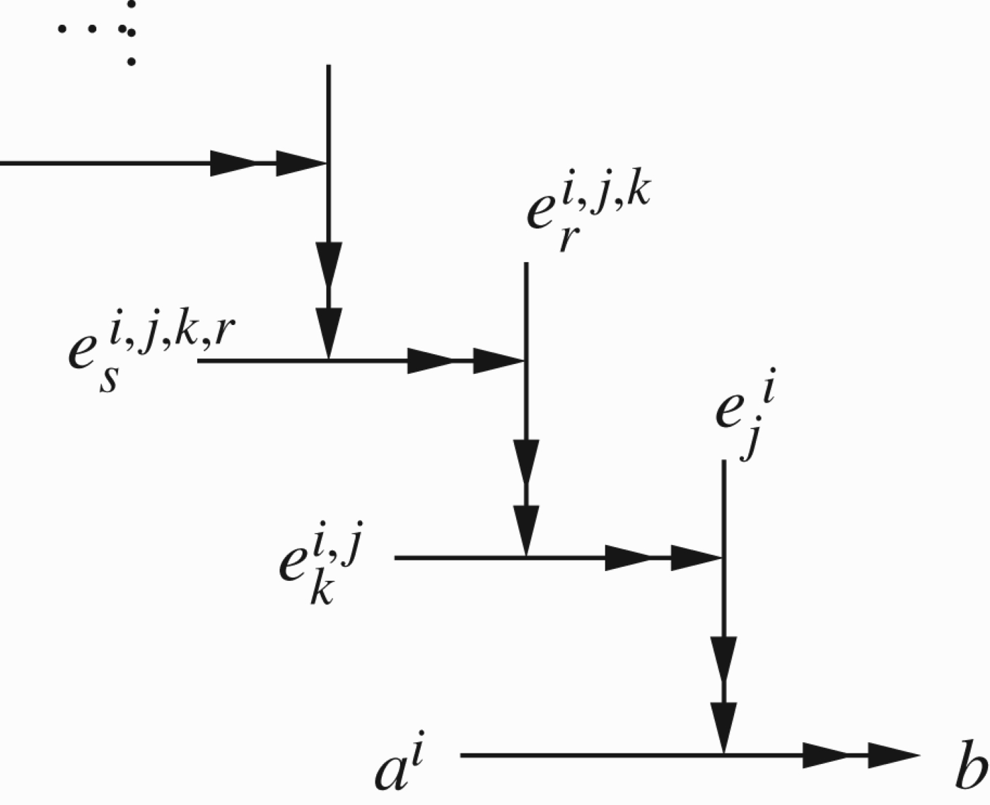
Figure 32.

A simple numerical attacks with transmission rate.

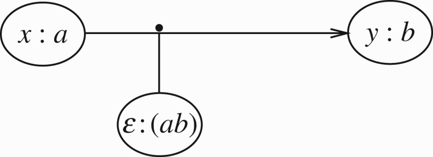
Figure 33.

A more complex numerical network.

Definition 4.3

Definition 4.3Higher level equations

Given a higher level network as in Definition 4.1, we define the equations for it in steps as follows:

Step 1. Insert a transmission factor ε(x,β) for every arrow of the form x↠β or of the form a→β in the network.
Step 2. View all higher order attacks on arrows as attacks on the transmission factor of the arrow. So the transmission factor becomes a sort of pseudo-node.
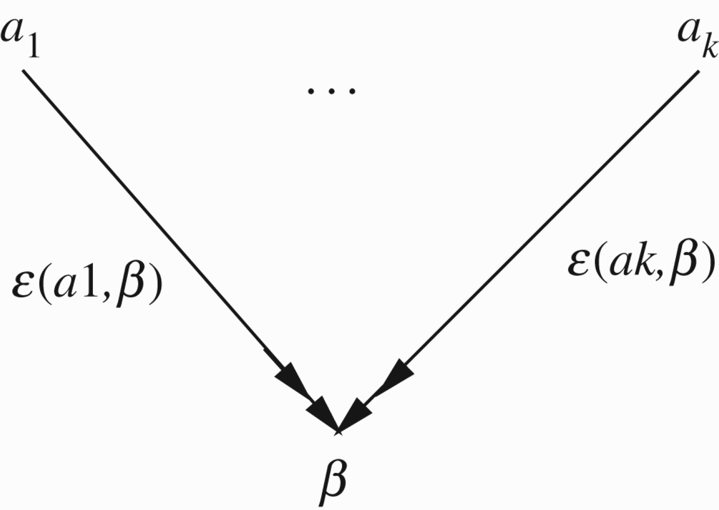
Step 3. For any pseudo-node β, whether it is a real node or a transmission factor, let Figure 34 represent all of attacks on it. The attack arrows have their own transmission factors as indicated in Figure 34. Note that for the purpose of writing the equations, transmission factors are not regarded as nodes. They are regarded as nodes only when they are attacked and play the role of β. Therefore, in Figure 34, the transmission factors are to be seen as such and not as pseudo-nodes.
We now have two options for equations.
Option HEqinverse(f):
f(β)=∏i=1k(1−f(ai)·f(ε(ai,β))).

Option HEqmax(f):
f(β)=1−maxi(f(ai)f(ε(ai,β))).
• Step 4. Solve the equations for the variables f(x), both for real nodes x and for transmission factors ε(x,y). All your solutions f represent all the extensions for the network.
If f(x)=1 then x= in.
If f(x)=0 then x= out.
If 0<f(x)<1 then x is undecided.

Figure 34.

Transmission factors can also be attacked.

This is a typical case for solving equational problems for variables f(b),b a node with the help of additional variables f(ε(a,b)), ε(a,b) a transmission factor. This idea for solving equations using additional variables is not new, it is hundreds of years old.

Remark 4.4

The perceptive reader will note the simplicity of our equations as compared with the complexity of the definitions of admissibility and extensions of Baroni, Hanh et al., Modgil and others!

Remark 4.5

Remark 4.5Baroni comment

The perceptive reader will further note that our current paper constitutes a positive response to a comment from Section 6 of Baroni et al. (2009):

The idea of encompassing attacks to attacks in abstract argumentation framework has been first considered in Barringer et al. (2005), in the context of an extended framework encompassing argument strengths and their propagation. In this quite different context, deserving further development, Dung style semantics issues have not been considered.

Example 4.6

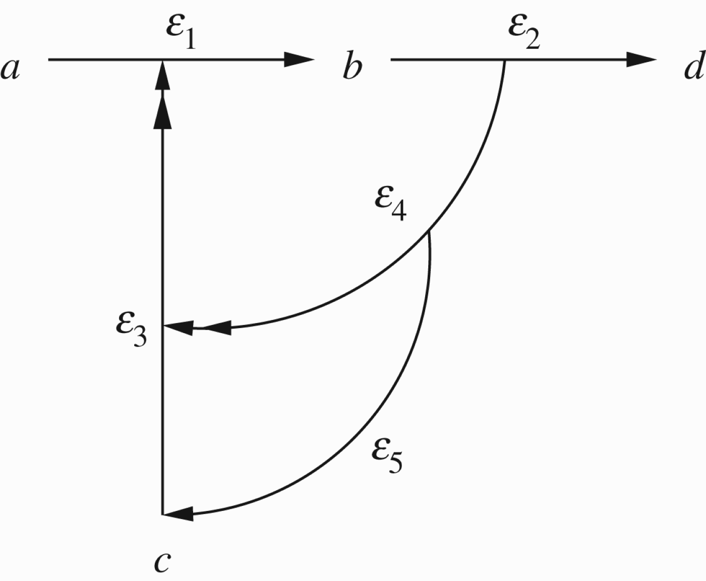
Let us do Figure 28. Use HEqinverse. First we add transmission. This can be seen in Figure 35.

The equations are:

(1) a=1 (not attacked).
(2) b=1−ε1a.
(3) d=1−bε2.
(4) ε2=1 (not attacked).
(5) ε3=1−ε4·ε2.
(6) ε4=1 (not attacked).
(7) ε1=1−cε3.
(8) c=1−ε4ε5.
(9) ε5=1 (not attacked).
Simplifying the equations, we get
(10) b=1−ε1.
(11) d=1−b.
(12) ε3=0.
(13) c=0.
(14) ε1=0.
The extension is
a=1,b=0,d=0,c=0.

Figure 35.

A network with attacks on transmission factors.

Example 4.7

Example 4.7Loop

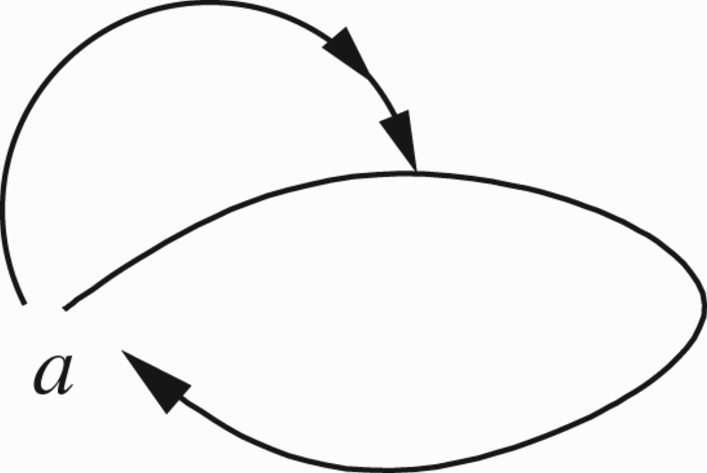
Consider Figure 36

Let ϵ be the transmission a→a.

The transmission a↠(a→a) is 1 since it is not attacked. We get again using HEqinverse:

(1) a=1−εa.
(2) ε=1−a.

a=1−(1−a)a,a=1−a+a2,a2−2a+1=0,a=1.

Thus, the extension is {a}.

Although a attacks itself, it also attacks its own attack and so a is in.

Figure 36.

A higher level self loop.

Example 4.8

Example 4.8Figure 1 from Hanh et al. 2010 entitled: A Bizzare framework

The previous Example 4.7 can be generalised as in Figure 37. This figure was put forward by Hanh et al. (2010) as an example showing how their approach to higher level attacks differs from Gabbay (2009c) and Baroni et al. (2009).

We quote from Hanh et al. (2010) (we adjust the figure references to ours here).

For illustration, consider a framework in Figure 37 consisting of attacks α₁=(A, A) and α_i+1=(A,α_i) for i≥1. It is rather hard to imagine any practical interpretation of this framework. Hence, as a sceptical reasoner, one would not want to draw any conclusion, i.e. does not accept A. An agent arguing for A has to rely on an infinite line of defence α₂,α₄…. The semantics of both Gabbay and Baroni et al. has a unique preferred extension<texlscub>A,α₂,α₄…</texlscub>, while our semantics has the empty set as the only extension. The example suggests that extended argumentation in a too literal form would allow counter-intuitive extensions.

Let us see what equations we get for our example.

Figure 37.

An infinite higher level self loop.

Case n= infinity from Figure 37, we get

(1) A=(1−A·α1).
(2) αn=(1−A·αn+1)

or equivalently

(1) α1=(1−A)/A.
(2) α2=(2A−1)/A2.
(3) α3=(A2−2A+1)/A3. …

We can see that A=1 is a solution.

Let us now continue to examine more cases, let us suppose that we have in Figure 37 only a finite number of higher level attacks.

Case n=3 The graph has the nodes {A,α1,α2,α3}.

What do we get?

Clearly α₃=1, since it is not attacked.

Hence, α2=1−A and

α1=(1−A(1−A)).

Therefore, we get

A=(1−A·α1)=(1−A·(1−A(1−A))).

We get the equation

A3−A2+2A−1=0.

There is a solution for A equals approximately around 0.5698402909980533, say A=0.57, and so we get α3=1,α2=0.43, and α1=0.755.

This means that all nodes can be taken as undecided except α₃.

Case n=4 The graph has the nodes {A,α1,α2,α3,α4}. Clearly α₄=1 since it is not attacked.

We have

α3=1−A,α2=1−A+A2,α1=1−A+A2−A3,A=1−A+A2−A3+A4.

(1) We have one solution A=1,α4=1,α3=0,α2=1,α1=0.
(2) There is also another solution of the degree 4 equation,
A=0.6823278038280193.

Again in this case, we get all nodes except the top α₄ are undecided.

Case n=m. In this case, the general equation for A is

A=1+∑fromk=1tok=m−1(−A)k.

Remark 4.9

Remark 4.9Support

The equations for higher level attacks allow us to interpret the notion of support in an equational way. Our interpretation of support in Section 3 was qualitative. We did not write equations for the support arrows but used them to define new attack relations (called threats) in Definition 3.1, and then wrote equations using the threat relation. So for example, we had nothing to say about Figure 17.

We can now put forward a new idea:

• Equational Support
a supports b if a attacks the transmission factor of any c attacking b

Thus, we read Figure 17 as Figure 38.

The equation for support is therefore

a=(1−x(1−y)).

Note that in this way we are lead to the notion of directed support. See next remark.

Figure 38.

A higher level representation of Figure 17.

Remark 4.10

Remark 4.10Directed support

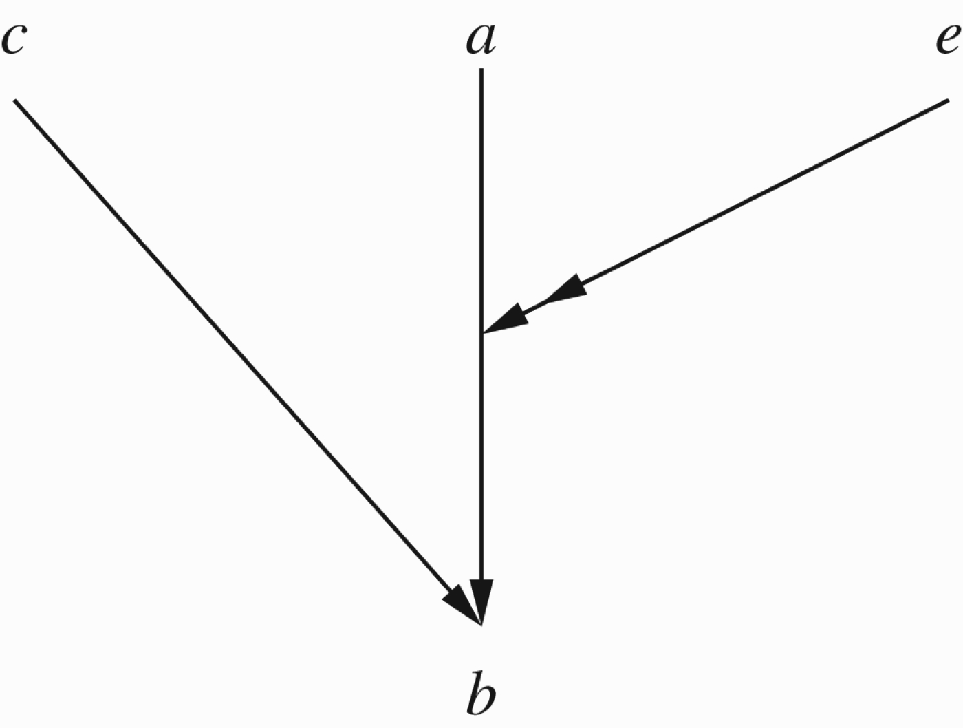
Let E be a set of arguments. Let e, b be arguments. e is the E directed support of the node b iff e attacks the transmission factor for any a∈E which attacks b.

Thus, Figure 39 would reduce to Figure 40.

We shall address directional equational support in the next section.

Figure 39.

Directed support.

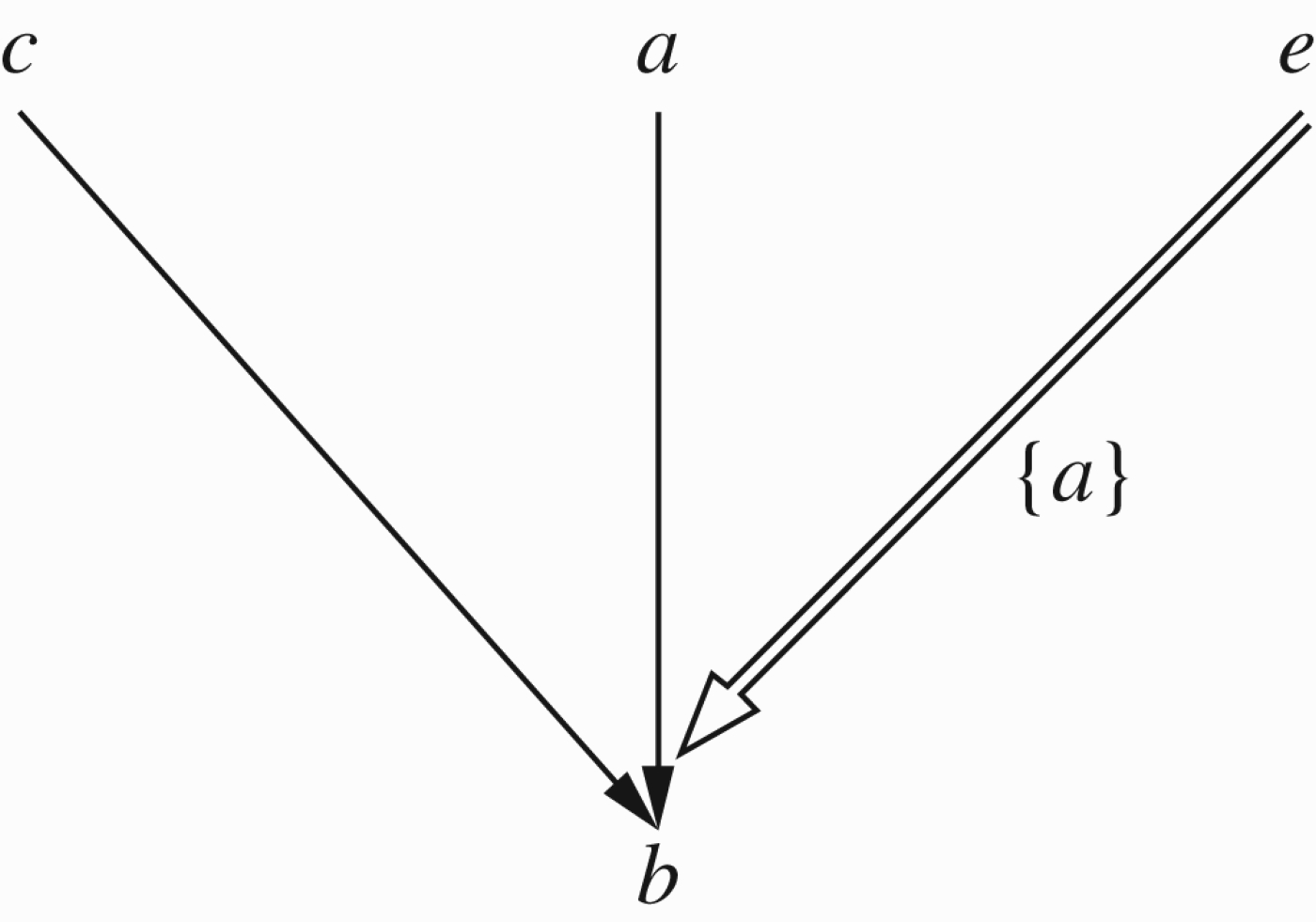
Figure 40.

Reducing directed support to higher level attack.

5.Approximately admissible extensions

A very natural next step in our equational approach is that of approximation. Whenever you have equations and their numerical solutions in mathematics, it is natural to examine approximations where certain aspects are neglected. In our case, the argumentation network is given equational semantics, the complete extensions sets are the solutions to the equations, therefore it is natural to look at the approximate solutions. What we get is a notion of approximate complete extensions. We can regard as being in those nodes getting a value near 1 (the notion of near needs to be defined) and to regard as being out those nodes getting a value near 0. Of course, these “approximate extensions” may not satisfy the usual constraints, e.g. a node may be undecided with an attacker being in (actually, approximately in), but we have to accept that.

We shall see that this section naturally relates to an important recent paper of Dunne, Hunter, McBurney, Parsons, and Wooldridge (2011).

Our starting point is Remark 1.6, where the notion of Admissible sets is changed to that of

• E is Suspect–Admissible if whenever a in E is attacked by c then either c is Suspect or E attacks c.

The above notion of Suspect was introduced in Remark 1.6 qualitatively using the loops in the attack relation, i.e. it is a geometrical notion.

If we are dealing with networks with transmission factors, as we have dealt extensively in Barringer et al. (2005), we can use the transmission factor to define the notion of Negligible

• The attack of node a on node b is Negligible if its transmission factor is very small.
• E is Approximately Admissible if whenever an element b in E is attacked by c then either the attack of c on b is Negligible or E attacks c via an attack which is not Negligible.

It is easy to see that the effect of using this notion is equivalent to disregarding all attacks with negligible transmission.

This immediately connects with Dunne et al. (2011), see their Definition 6.

In fact from our point of view where extensions are solutions of equations, the notion of Approximate Admissibility is automatically taken care of by the equations, because for a very low transmission factor ϵ of x attacking y, the expression ϵ. x which appears in the equations, is very near zero and has almost no effect on the equations.

Thus, the correct notion for us is to take as in not just the points x for which f(x)=1, but also points where the value of f is very near 1.

Frankly, there is not much more to say about this, except to compare with Dunne et al. (2011).

Dunne et al. (2011) have not used any of the machinery of Barringer et al. (2005). In Barringer et al. (2005), networks had transmission values (corresponding to weights) and calculations and propagations of values were performed, with extensive study of the influence of loops.

They say in their paper and I quote:

So, whilst there is gathering momentum for representing and reasoning with the strength of arguments or their attacks, there is not a consensus on the exact notion of argument strength or how it should be used. Furthermore, for the explicit representation of extra information pertaining to argument strength, we see that the use of explicit numerical weights is under-developed. So, for these reasons, we would like to present weighted argument systems as a valuable new proposal that should further extend and clarify aspects of this trend towards considering strength, in particular the explicit consideration of strength of attack between arguments.

I saw their paper a few months ago just before it was going into print. I contacted the authors and I am grateful that they managed some last minute adjustments of their text.

We include one example comparing our approximation approach with that of Dunne et al. (2011).

Example 5.1

Example 5.1Dunne et al. 2011, Figure 2

We show the connection by treating Dunne et al. (2011, Figure 2) using our system.

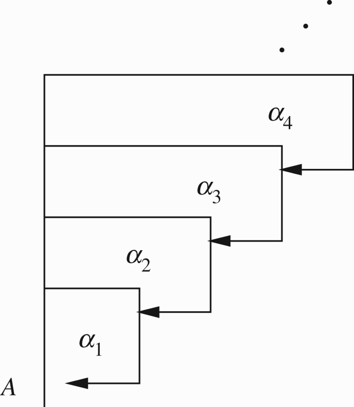
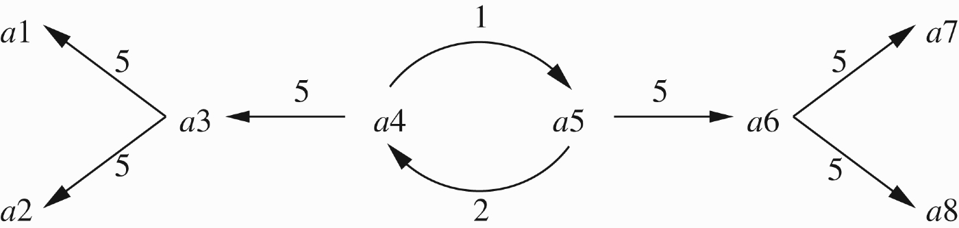
Consider Figure 41

In Figure 41, the weights are from the numbers x from the set {1,2,3,4,5}. They become in our system transmission values, which are numbers y from [0, 1]. So the simple transformation y=x/5 will change the weights to fractions of the maximal weight 5.

Now looking at Figure 41 with weights adjusted, clearly the problem is the loop

a4→a5 with strength 1/5

and

a5→a4 with strength 2/5.

The equations just for this loop are therefore

a5=(1−0.2a4).a4=(1−0.4a5).

The solution is

a4=30/46.a5=40/46.

the other values are easily calculated to be

a6=(1−a5)=6/46.a7=a8=(1−a6)=40/46.a3=(1−a4)=16/46.a1=a2=(1−a3)=30/46.

If we take the approximate extension E of all nodes of values from 40/46, we get E={a5,a7,a8}.

If we take the approximate extension E′ of all nodes of values from 30/46, we get E′={a1,a2,a4,a5,a7,a8}.

E corresponds to disconnecting the attack of a4 on a5 and E′ corresponds to also disconnecting the attack of a5 on a4.

This is in full agreement with Dunne et al. (2011).

Figure 41.

A weighted network.

Remark 5.2

Remark 5.2Advantages of our method over Dunne et al. 2011

We now list the advantages of our method over Dunne et al. (2011). First advantage is that we can approximate without weights. Consider the loop of Example 1.10. Here, we have no weights and no transmissions. The numbers come from the equations, yet because we have numbers we can approximate.

Second advantage is that there are approximations which are not generated by weights and cancelled links, but only from numbers. Some numbers arise from multiple attacks. Some numbers come from the equations.

Most importantly, when we accept nodes with numbers near 1 as “in”, we are not changing the values of other nodes!

So, for example, in Example 1.10 and Figure 9, we can accept node c as “in” on account of it being the only one with a value more than 0.5, but this does not make the value of node a 0.

Note by the way that {c} is he only Suspect–Admissible extension when we consider nodes a and b as Suspect on account of their attacking themselves.

A much more important application of these approximations is the handling of loops.

6.The equational view of semantics (preferred, stable, semi-stable, grounded)

This section deals with numerical and computational aspects of our equational models, and how they can calculate semantic extensions.

We begin with options for calculating extensions in ordinary Dung networks and their comparison with Caminada labelling. Our embarkation point is a table from Caminada and Gabbay (2009).

See Table 1.

Table 1.

Argument labellings and Dung-style semantics.

Restriction complete labellings	Dung-style semantics	Linked by definition and theorem of Caminada and Gabbay (2009)
No restrictions	Complete semantics	Def. 5 and Th. 1
Empty undec	Stable semantics	Def. 8 and Th. 5
Maximal `in`	Preferred semantics	Def. 10 and Th. 7
Maximal `out`	Preferred semantics	Def. 10 and Th. 7
Maximal undec	Grounded semantics	Def. 9 and Th. 6
Minimal `in`	Grounded semantics	Def. 9 and Th. 6
Minimal `out`	Grounded semantics	Def. 9 and Th. 6
Minimal undec	Semi-stable semantics	Def. 11 and Th. 8

We now write equations whose solutions give the correct extensions. We assume a set of equations Eq which is sound for Dung semantics, such as offered in Definition 1.1.

Our network is (S, R_A). Assume, in case we want to refer to the points of S explicitly, that S={x1,…,x(n+k)}.

We begin with a word of explanation and orientation addressed to the perceptive reader. In the set theoretic context of Dung extensions and semantics, there is uniformity and beauty in defining the semantics and the extensions, in terms of maximality and minimality of complete admissible sets. One can also define new types of semantics such as CF2 or stage or ideal or sceptical semantics, again using set theoretic concepts such as conflict freeness and intersections of extensions.

So, for example, a preferred extension is defined as a maximal complete extension.

When we move to the world of equations, we can get the basic complete extensions as functions f which are solutions to equations. We can still talk about maximal or minimal functions relative to point-wise numerical ordering. Thus, we can define a preferred solution f as a maximal solution to the equations.

However, in the context of equations, we are tempted to use further equations and constraints and get the semantics directly as solutions of equations with constraints. This can get messy and we lose uniformity.

What we gain is that we can use solvers to find the maximal solutions.

What we lose, for example, is that we cannot form infinite products of functions, which correspond to infinite intersections of extensions.

Note also that if we use equations which are different from Eq_max, we obtain something not corresponding to Dung complete semantics, but something analogous to it for the type of equations used. Let us call it pseudo-complete semantics. Then, it may be interesting to investigate notions like pseudo-stable or pseudo-grounded semantics in a purely numerical context. We leave this to future work.

Case complete extensions. Solve the Eq_max equations. Any solution f is an extension.

Case stable extensions. Add a new variable y such that y ¬∈S, and write the additional equation

f(y)=hy=∑x∈Sf(x)(1−f(x)).

If the solution f to the new expanded set of equations is a stable extension, then f(x)(1−f(x)) is 0 for all x∈S and hence f(y)=0. Conversely, if f(y)=0 then f is stable. Thus, to check for stable extensions, we check f(y).5 5

Case of semi-stable extensions. This case minimises the undecided. We do the following.

Consider the quantity

μ=∑a∈Sx1,…,xn∈Sare allattackers ofa[a−ha(x1,…,xn)]2.

In μ we regard all elements of S as variables. The equation μ=0 has a solution. We regard μ=0 as a constraint and minimise the expression

ν=∑x∈Sx(1−x)

subject to the constraint μ=0.

This can be done using the method of Lagrange multipliers (see Wikipedia).

Case of grounded extensions. This is like the semi-stable case except that we minimise the expression 1−ν.

Remark 6.1

Remark 6.1Connection with the intertranslatability of argumentation semantics

In a brilliant recent paper, Dvorak and Woltran (2011) investigate translations of one type of extension into another. This has bearing to this section together with our notion of Critical Translations (Definition 2.9 in Section 2.2).

7.Time-dependent networks

There are two ways to make a system time dependent.

(1) Make each atomic component depend on time.
(2) Take snapshots of the system at different times.

If we follow the first method for the case of argumentation networks, we will make each argument strength time dependent and the transmission factors also time dependent. So, for example, if we look again at Figure 32 as a typical figure, and make it time dependent, then the coefficients x: a and y: b become time dependent, as does the transmission factor ε:(ab). This is how we already presented time dependence in Barringer et al. (2005). Thus, we have x(t,a),y(t,b),ε(t,a,b), where t is a time variable.

If we follow the second approach, we again use a time variable t but our networks have the form (S_t, R_{A, t}), where RA,t⊆St.

The first approach is more general. We can take a time-dependent model of the first approach and get from it a model of the second approach. If we allow x(t) and ε(t) to take only {0,1} values, we can let

St={a|x(t,a)=1},RA,t={(a,b)|x(t,a)=y(t,b)=ε(t,a,b)=1}.

Thus, we get a model (S_t, R_{A, t}) according to the second approach.

Note that if we do not involve the time element in the equations of the attack, all we would have is lots of non-interacting networks sitting around. So to get some interaction, let us review the basic temporal configurations and the options they afford us.

Figure 42 is a typical situation, we allow for three nodes for simplicity.

Figure 42.

A typical temporal attack configuration.

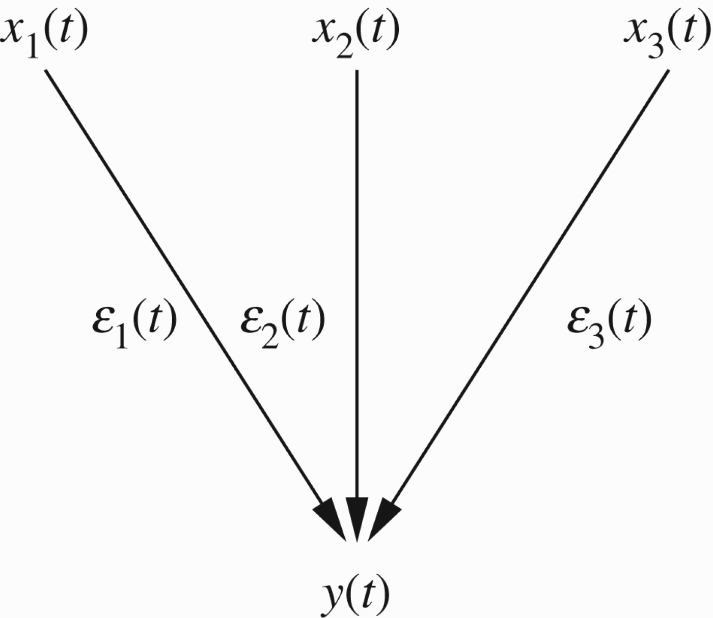
Let us assume that 0⩽xi,εj⩽1 and also that 0≤t≤1, so that we shall always have solutions to our equations. The value y(t) depends on xi(t),εi(t) as in Definition 4.3.

y(t)=(1−x1(t)ε1(t))(1−x2(t)ε2(t)(1−x3(t)ε3(t))).(∗)

Let

αi(t)=(1−xi(t)εi(t)),

where α_i(t) is the effective attack of node x_i(t). The total attack is

y(t)=∏iαi(t).

We want to modify α_i(t) in view of the time dependence.

Equation (*) does not express any interaction in time. Suppose we want to add some temporal interactions, what option can we offer?

7.1.Option

We can make the attract at time t depend also on the rate of change at t.

Surely if the strength of the attack is on the decline, it is less effective. So we can look at the derivatives dxi(t)/dt and dεi(t)/dt and look at their value at the point t.

If the rate is increasing, we make the attack of x_i(t) on y a bit stronger, otherwise a bit weaker.

Imagine that you are trying to buy a house and the price of the house is attacking the argument that you should own your house (rather than rent). If prices are going up, the argument for buying now is stronger. If they are going down, it is weaker, all compared with a temporal situation where prices are not changing.

Let us use the same notation that is used in physics. ẋ_i (t) is the value of the definative at t. Similarly ε˙j(t).

Define r_i(t) and s_i(t) as follows.

(1) If x˙i(t)=0, let r_i(t)=1.
If x˙i(t)>0, let ri(t)=1/(1+1/x˙i(t)).
If x˙i(t)<0, let ri(t)=1/(1−1/x˙i(t)).
So ri(t)=1/(1+1/|x˙i(t)|).
Define s_i(t) similarly using ε˙i(t).
Now consider the attack x_i(t) on y(t). We want to modify the original expression
α1(t)=[1−xi(t)εi(t)]
into a new expression β_i(t) and use that to define the attack. Clearly, if we think the force of the attack is going to decline, then the attack should be less effective. Thus, for example, if ẋ_i(t) is very large and negative, this means that the attack of x_i is going down very quickly and r_i(t) is almost 1. We can almost ignore the attack. So, we multiply x_i(t) by 1−r_i(t). Thus, we get
βi(t)=1−xi(t)εi(t)(1−ri(t)).
Since 1−r_i(t) is almost 0, we get that β_i(t) is almost 1, thus we are almost ignoring this attack. If x˙i(t)>0 and is very large, again r_i(t) is almost 1 but the attack of x_i is strengthened. So, we multiply α_i by (1−r_i(t)), and the attack becomes stronger. βi(t)=αi(t)(1−ri(t)). Similarly, if εi(t)<0, this means transmission is going down so, we multiply εi(t) by (1−s_i(t)). If ε˙i(t)>0, then εi(t) is going up, then we multiply α_i by (1−s_i(t)). So, this defines β_i(t) and we let
ynew(t)=∏iβi(t).
To take an example, assume for simplicity that the transmission factor is constant in time but that x(t) declines exponentially in [0, 1]. Let
xi(t)=e−t.
Therefore,
αi(t)=(1−εe−t)
and
ri(t)=11+e−t,
and so
1−ri(t)=11+et.
We therefore have
βi(t)=1−εe−t1+et.
So, the attack is less effective!

7.2.Final comment

The equational approach allows us to take into consideration the rate of change of the strength of the attacks. This is not possible or even expressible in the traditional Dung networks.

Let us now see what options we have in the snapshot approach. To simplify, let us assume three points of time, and simple networks, as in Figure 43.

Figure 43.

Temporal snapshot approach.

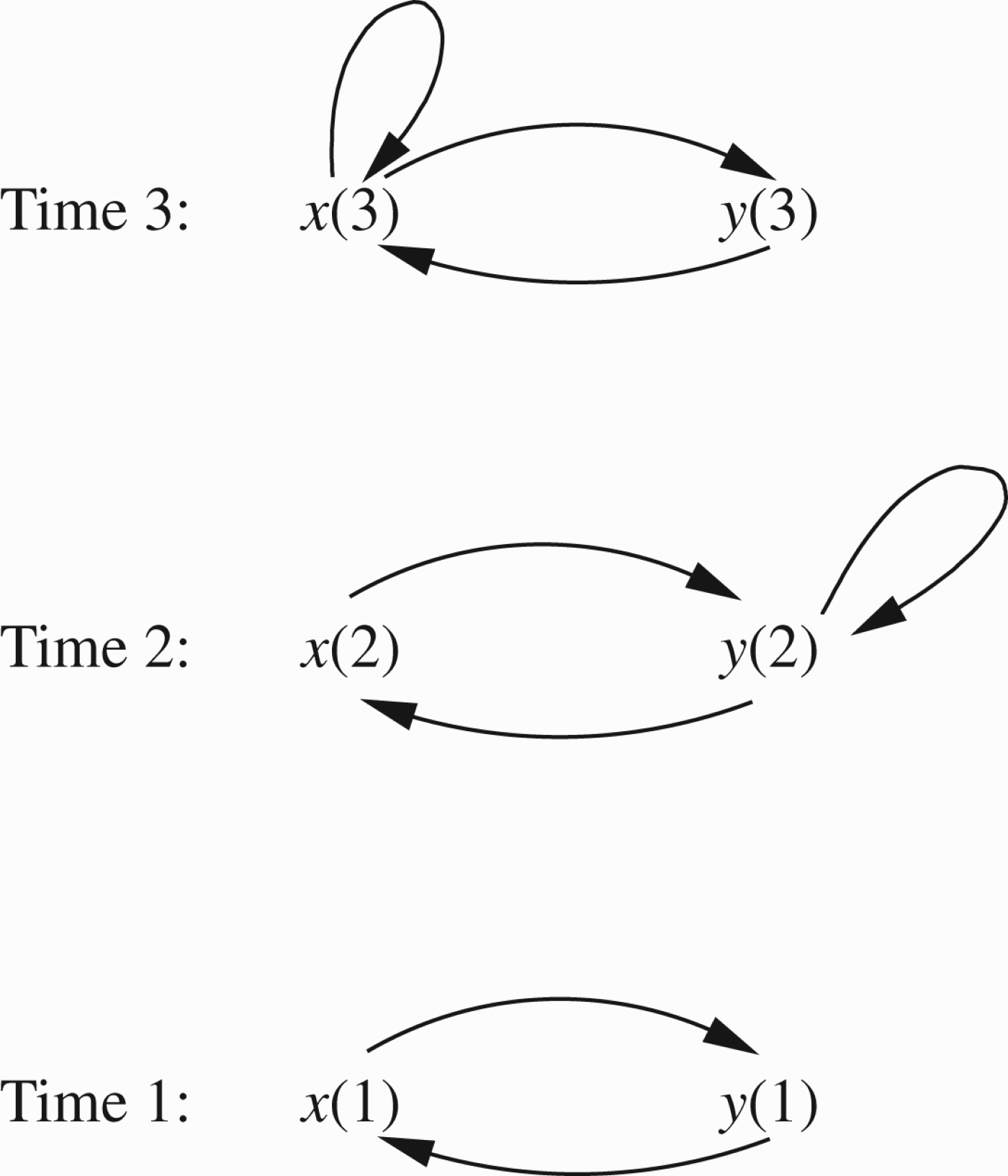
Note the following:

(1) If there is no connection between the times, then this is just a flat network without regard to time.
(2) Even if we add attacks from future to past, e.g. x(2)→y(1) then it is still a flat network.

The only way is to say that, for example

y(1)=(∃t>1)y(t).

So we have an existential quantifier here and y(1) is say “in” if some y(t) for t>1 is “in” or, if we are writing equations then we might have, for example

y(1)=(1−x(1))1−max(t>1){y(t)}.

The reader can see that this approach is different from the previous “rate of change” approach.

This approach is investigated in my paper with Gabbay and Modgil (2009). See also my paper with Barringer and Gabbay (2010).

8.Conclusion and future work

Discussion

Let us put forward how we see the results of this paper. This is my personal view and it explains the methodology of this paper.

There are several areas in logic where major monotonic and fixed point operations take place. For example,

(1) Logic programming, where the content of the logic programme is determined by fixed points of suitable monotonic operations on the Herbrand universe.
(2) Pure logic (e.g. classical or Ł ukasiewicz logics), where the deductive closure of theories is determined by fixed points of the consequence operations.
(3) Default logics, autoepistemic logics and the like where the extensions are defined as fixed points of certain operations. In each of the above areas, let us identify roughly two major “components”.
- (a) The unit operational concepts.
- (b) The fixed point extensions as defined using (a).
In logic programming, (a) is the Horn clause and negation as failure. In pure logic, (a) is the notion of proof rules (or immediate consequence). In default logic, (a) is the default rule. (b) is more or less defined using (a) in a predictable way. In the year 1995, Dung (1995) came with another area:
(4) Argumentation frames.

His basic concept (a) was attack and admissibility, and using that he defined fixed points and extensions. His seminal paper contains more. He identified his own (a) notions in the (a) notions of default logic and in logic programming and thus was able to present default logic and logic programming in the framework of argumentation.

In my view all of these areas, (1)–(4) belong to the same family of systems and share a set-theoretic fixed point approach.

Being in the same family manifests itself also in the predictability and ease of translation from one system (of (1)–(4)) to the other. This was already pointed out in Gabbay (2009a,b) and Gabbay and d'Avila Garcez (2009) and in Sections 2.2 and 8.2 of this paper. It was also pointed out by other researchers, such as Brewka and Woltran (2010) and Brewka et al. (2011).

In fact in my very recent paper (Gabbay), I show that Dung argumentation theory has the power of classical propositional logic, and this of course explains its expressive power.

The equational approach is a different family. It has its root in the early nineteenth century and it is not set theoretic. The fixed point feature does manifest itself in the equational approach through Brouwer's fixed point theorem, but otherwise the equational approach can go in different directions. We now elaborate on these new directions:

(1) Connections with other purely numerical networks such as flow or ecology networks.
(2) The extensions in the set-theoretic family are the solutions to equations in the equational approach. The equations can be solved in different ways.
- (a) We can impose constraints.
- (b) We can insist on the solutions to follow certain algorithmic restrictions.
  We already saw that we need this to implement defaults, but we also can get new results in Logic, as shown in D'Agostino and Gabbay (2011).
(3) We can approximate solutions, as we mention in Section 5 of this paper.

8.2.Comparison with other papers

Some initial results are put forward to Gratie and Maqda Florea (2011) in the preliminary submission. In communication with them, it appears that they were not aware of Gabbay (2009b). Also translations into argumentations networks, like the ones in Sections 2.2, were already introduced in Gabbay's (2009b) paper and independently in Brewka et al.’s (2011) paper. For further development of the Equational idea see Gabbay, D.M. (2012c), ‘The Equational Approach to CF2 Semantics’, to appear in COMMA 2012.

Gabbay, D.M. (2012d), ‘The Equational Approach to Logic Programs’, to appear in LNCS 7265 Festschrift for Vladimir Lifschitz, eds. E. Erdem, J. Lee, Y. Lierler, and D. Pearce, pp. 279–295.

Gabbay, D.M. (2012e), ‘What is Negation as Failure Paper Written in 1985’, revised version published in Sergot Festschrift, eds. A. Artikis et al., LNAI 7360, Heidelberg: Springer, pp. 52–78.

Gabbay, D.M. Meta-Logical Investigations in Argumentation Networks, Research Monograph for Springer.

Notes

1 The other solutions are

[(1−5)±i10+25]/4,[(1−5)±i10−25]/4.

2 See http://en.wikipedia.org/wiki/Brouwer_fixed_point_theorem (Sobolev 2001).

3 We have in these papers not only weighted nodes (arguments) and weighted arrows (attacks), but also higher level attacks, temporal dependence, and a lot more. These notions are being reproduced now by many authors. See, for example, Baroni, Cerutti, Giacomin, and Guida (2009) and Dung (1995) for higher level attacks originating in Barringer et al. (2005), and our discussions and further development in Gabbay (2009a,b,c). These papers are part of a general methodological approach to applied logic and connect many areas together.

4 Hanh et al. point out that their approach is sceptical generalisation of the standard argumentation framework, while others such as Sanjay's, Gabbay's, or Baroni et al.’s are rather credulous. Hence, in each extension of these approaches, there is a sceptical part that is one of Hanh et al.’s extensions. Hanh et al. also point out that Sanjay's generalisation of grounded semantics is rather more liberal than theirs, and hence his characteristic function is not monotonic.

5 This is a neater condition than the one mentioned in Remark 2.19, which was more explanatory than efficient.

Acknowledgements

I am grateful to Martin Caminada, Nachum Dershowitz, Phan Minh Dung, David Makinson, Alex Rabinowich, and Serena Villata for helpful discussions. I am also indebted to the referees for their penetrating comments and methodological criticisms. Research done under ISF project: Integrating Logic and Network Reasoning.

References

1	Baroni, P., Giacomi, M. and Guida, G. (2005) . SCC-Recursiveness: A General Schema for Argumentation Semantics. Artificial Intelligence, 168: (1–2): 162–210.
2	Baroni, P., Cerutti, F., Giacomin, M. and Guida, G. (2009) . “Encompassing Attacks to Attacks in Abstract Argumentation Frameworks”. In ECSQARU, Edited by: Sossai, C. and Chemello, G. 83–94. Springer. Lecture Notes in Computer Science 5590
3	Baroni, P., Cerutti, F., Dunne, P. E. and Giacomin, M. Computing with Infinite Argumentation Frameworks: The Case of AFRAs. Proceeding TAFA’11 Proceedings of the First international Conference on Theory and Applications of Formal Argumentation. Berlin. pp. 197–214. Heidelberg: Springer-Verlag.
4	Barringer, H. and Gabbay, D. M. (2010) . “Modal and Temporal Argumentation Networks’, in the Amir Pnueli Memorial Volume”. In Time for Verification, Edited by: Peled, D. and Manna, Z. 1–25. Berlin, Heidelberg: LNCS, Springer.
5	Barringer, H., Gabbay, D. M. and Woods, J. (2005) . “Temporal Dynamics of Argumentation Networks”. In Mechanising Mathematical Reasoning, Edited by: Hutter, D. and Stephan, W. 58–98. Berlin, Heidelberg: Springer. LNCS 2605
6	Barringer, H., Gabbay, D. M. and Woods, J. (2008) . “Network Modalities”. In Linguistics, Computer Science and Language Processing. Festschrift for Franz Guenthner on the Occasion of his 60th Birthday, Edited by: Gross, G. and Schulz, K. 79–102. London, UK: College Publications.
7	Barringer, H., Gabbay, D. M. and Woods, J. (2012) . Temporal, Numerical and Meta-Level Dynamics in Argumentation Networks. Argument and Computation, 3: (2–3) (to appear).
8	Bench-Capon, T. J.M. (2003) . Persuasion in Practical Argument Using Value-Based Argumentation Frameworks. Journal of Logic and Computation, 13: : 429–448.
9	Boella, G., Gabbay, D. M., van der Torre, L. and Villata, S. (2010) . “Support in Abstract Argumentation”. In Computational models of Argument, COMMA 2010, Edited by: Baroni, P., Cerutti, F., Giacomi, M. and Simari, G. 111–122. Amsterdam: IOS Press.
10	Boella, G., Gabbay, D. M., van der Torre, L. and Villata, S. (2011) b. “Support in Abstract Argumentation”. In Expanded Version for Annals of Mathematics and Artificial Intelligence, 2012, Berlin, Heidelberg: Springer Verlag. to appear.
11	Boole, G. (1847) . The Mathematical Analysis of Logic Macmillan, Barclay, & Macmillan; London: George Bell, 1847, Cambridge and London.
12	Brewka, G. and Woltran, S. (2010) . “Abstract Dialectical Frameworks”. In Proceedings of Twelfth International Conference KR 2010, 02–111. Chicago and London: AAAI Press. KR-2010, 2010
13	Brewka, G., Dunne, P. and Woltran, S. (2011) . “Relating the Semantics of Abstract Dialectical Frameworks and Standard AFs”. In Proceedings of Twenty-Second International Joint Conference on Artificial Intelligence (IJCAI-11), 780–785. Palo Alto, California: AAAI press.
14	Caminada, M. and Gabbay, D. M. (2009) . A Logical Account of Formal Argumentation. Studia Logica, 93: (2–3): 109–145.
15	Caminada, M. and Wu, Y. On the Limitations of Abstract Argumentation. Proceedings of BNAIC 2011; the 23rd Benelux Conference on Artificial Intelligence. November 3–4 2011, Ghent, Belgium. Edited by: De Causmaecker, P., Verbeeck, K., Maervoet, J. and Messelis, T. pp. 69–66.
16	Cayrol, C. and Lagasquie-Schiex, M. C. (2005) . “On the Acceptability of Arguments in Bipolar Argumentation Frameworks”. In ECSQARU, Lecture Notes in Computer Science 3571 Edited by: Godo, L. 378–389. Berlin, Heidelberg: Springer.
17	Cayrol, C. and Lagasquie-Schiex, M. C. (2010) . Coalitions of Arguments: A Tool for Handling Bipolar Argumentation Frameworks. International Journal of Intelligent Systems, 25: (1): 83–109.
18	Couturat, L. (1914) . The Algebra of Logic, Chicago and London: Open Court.
19	D'Agostino, M. and Gabbay, D. (2011) . “Depth-Bounded Logics 1”. In Equational Nets for Classical and Paraconsistent Reasoning with Arbitrary Boolean Operators Paper 425. 1st draft, April 18, 2011.
20	Dung, P. M. (1995) . On the Acceptability of Arguments and its Fundamental Role in Non-Monotonic Reasoning, Logic Programming and n-Person Games. Artificial Intelligence, 77: : 321–357.
21	Dunne, P., Hunter, A., McBurney, P., Parsons, S. and Wooldridge, M. (2011) . Weighted Argument Systems. Artificial Intelligence, 175: : 457–486.
22	Dvorak, W. and Woltran, S. (2011) . On the Intertranslatability of Argumentation Semantics. Journal of Artificial Intelligence Research, 41: : 445–475.
23	Gabbay, D. M. (2008) . “Reactive Kripke Semantics and Arc Accessibility”. In Pillars of Computer Science: Essays dedicated to Boris (Boaz) Trakhtenbrot on the Occasion of his 85th Birthday, Edited by: Avron, A., Dershowitz, N. and Rabinovich, A. 292–341. Berlin, Heidelberg: Springer-Verlag. Earlier version of this paper was published in Proceeding of CombLog04 http://www.cs.math.ist.utl.pt/comblog04/, eds. W. Carnielli, F.M. Dionesio, and P. Mateus, Centre of Logic and Computation University of Lisbon 2004, pp. 7–20. ftp://logica.cle.unicamp.br/pub/e-prints/comblog04/gabbay.pdf
24	Gabbay, D. M. (2009) a. Provability Foundations for Argumentation Networks. Studia Logica, 93: (2–3): 181–198.
25	Gabbay, D. M. (2009) b. Fibring Argumentation Frames. Studia Logica, 93: (2–3): 231–295.
26	Gabbay, D. M. (2009) c. Semantics for Higher Level Attacks in Extended Argumentation Frames Part 1: Overview. Studia Logica, 93: : 355–379.
27	Gabbay, D. M. Introducing Equational Semantics for Argumentation Networks. Proceedings of ECSQARU’11. Berlin. pp. 19–35. Heidelberg: Springer-Verlag. LNAI 6717
28	Gabbay, D. M. (2012) a. “The Equational Approach to CF2 Semantics”. February 2012, arXiv:1203.0220v1 [cs.AI].
29	Gabbay, D. M. (2012) b. “Linear Logic loop Checker for Handling Odd Loops in Argumentation Networks”. February 2012, paper 461.
30	Gabbay, D. M. (2012) c. The Equational Approach to CF2 Semantics. to appear in COMMA 2012.
31	Gabbay, D. M. (2012) d. “The Equational Approach to Logic Programs’, to appear in LNCS 7265”. In Festschrift for Vladimir Lifschitz Edited by: Erdem, E., Lee, J., Lierler, Y. and Pearce, D. 279–295.
32	Gabbay, D. M. (2012) e. “What is Negation as Failure Paper Written in 1985’, revised version published in Sergot Festschrift ”. Edited by: Alexander, Artikis, Robert, Craven, Kesim Cicekli, Nihan and Sadighi, Babak. 52–78. Kostas Stathis: Logic Programs, Norms and Action – Essays in Honor of Marek J. Sergot on the Occasion of His 60th Birthday Springer 2012, LNAI 7360, Heidelberg: Springer
33	Gabbay, D. M. (2011) . Dung's Argumentation is Essentially Equivalent to Classical Propositional Logic with the Peirce-Quine Dagger. Logica Universalis, 5: (2): 255–318. DOI:10.1007/s11787-011-0036-3.
34	Gabbay, D. M. Meta-Logical Investigations in Argumentation Networks, Research Monograph for Springer under contract.
35	Gabbay, D. M. and Modgil, S. (2009) . Modal Argumentation, Draft, May 2009.
36	Gabbay, D. M. and d'Avila Garcez, A. (2009) . Logical Modes of Attack in Argumentation Networks. Studia Logica, 93: (2–3): 199–230.
37	Gabbay, D. M. and Szał as, A. (2009) . Annotation Theories Over Finite Graphs. Studia Logica, 93: (2–3): 147–180.
38	Gratie, C. and Maqda Florea, A. Fuzzy Labelling for Argumentation Frameworks. ArgMas2011, 8th International Workshop on Argumentation in Multi-Agent Systems. May 2011, Taipei, Taiwan. pp. 18–25.
39	Hanh, D. D., Dung, P. M. and Thang, P. M. (2010) . “Inductive Defence for Sceptical Semantics of Extended Argumentation”. In Journal of Logic and Computation, Vol. 21 2: , 307–349. Oxford, UK: Oxford University Press. April 2011
40	Modgil, S. An Abstract Theory of Argumentation that Accommodates Defeasible Reasoning about Preferences. Proceedings of 9th European Conference, ECSQARU 2007. October 31–November 2 2007, Hammamet, Tunisia. pp. 648–659. Springer. Lecture Notes in Computer Science 4724
41	Modgil, S. (2009) . Reasoning About Preferences in Argumentation Frameworks. Artificial Intelligence, 173: : 901–993.
42	Schröder, E. Vorlesungen über die Algebra die Logik (3 vols) , 1890–1904. Leipzig: B.G. Tuebner. Reprints, Chelsea, 1966; Thoemmes Press, 2000.
43	Sobolev, V. I. (2001) . “Brouwer Theorem’, in Hazewinkel, Michiel”. In Encyclopaedia of Mathematics, Berlin, Heidelberg: Springer.
44	Wu, Y., Caminada, M. and Gabbay, D. (2009) . Complete Extensions in Argumentation Coincide with 3-Valued Stable Models in Logic Programming. Studia Logica, 93: (2–3): 381–401.

Abstract

1.Introduction

1.1.Aims of this paper

1.2.The conceptual vs. computational distinction

Figure 1.

Figure 2.

Figure 3.

1.3.Equational examples

Definition 1.1

Definition 1.1Possible equational systems

Example 1.2

Example 1.3

Example 1.4

Example 1.5

Remark 1.6

Example 1.7

Example 1.8

Example 1.9

Example 1.9Caminada labelling and the Max function

Example 1.10

Example 1.11

Example 1.11Comparing Eqmax and Eqinverse

Example 1.12

1.4.More on what equations can do

Example 1.13

Example 1.13Boolean functions, Abstract dialectical framework of Brewka and Woltran 2010

Remark 1.14

Remark 1.14Order among attackers

2.Formal theory of the equational approach to argumentation networks

Figure 4.

Figure 5.

Figure 6.

2.1.Real numbers equational networks

Definition 2.1

Definition 2.1Real equational networks

Theorem 2.2

Theorem 2.2Existence theorem, the finite case

Proof

Remark 2.3

Remark 2.4

Remark 2.5

Remark 2.5Existence theorem for the infinite finitary case

Lemma 2.6

Theorem 2.7

Theorem 2.7Caminada complete labelling functions and Eqmax

Proof

Remark 2.8

Remark 2.8Caminada complete labelling and Eqinverse

2.2.Critical translations of logic programmes and Boolean networks

Definition 2.9

Definition 2.9Critical subsets

Remark 2.10

Example 2.11

Example 2.11Critical translation for logic programmes and Boolean nets

Construction 2.12

Example 2.13

Remark 2.14

Remark 2.14Equations for logic programmes

Remark 2.15

Remark 2.15Embedding logic programmes into argumentation networks

Remark 2.16

Remark 2.17

Remark 2.17Discussion of Brewka and Woltran 2010

Remark 2.18

Remark 2.19

Remark 2.19Finding extensions

3.Analysis of support

3.1.Caution about support

Figure 7.

Figure 8.

Figure 9.

Figure 10.

Figure 11.

Figure 12.

Figure 13.

3.2.Equational model of support

Figure 14.

Figure 15.

Figure 16.

Figure 17.

Example 1.11Comparing Eq_max and Eqinverse

Theorem 2.7Caminada complete labelling functions and Eq_max