
Wealth management: Modeling the nonlinear dependence
Abstract
This work aims at the development of an enhanced portfolio selection method, which is based on the classical portfolio theory proposed by Markowitz (1952) and incorporates the local Gaussian correlation model for optimization. This novel method of portfolio selection incorporates two assumptions: the non-linearity of returns and the empirical observation that the relation between assets is dynamic. By selecting ten assets from those available in Yahoo Finance from S&P500, between 1985 and 2015, the performance of the new proposed model was measured and compared to the model of portfolio selection of Markowitz (1952). The results showed that the portfolios selected using the local Gaussian correlation model performed better than the traditional Markowitz (1952) method in 63% of the cases using block bootstrap and in 71% of the cases using the standard bootstrap. Comparing the calculated Sharpe ratios, the proposed model yielded a better adjusted risk-return in the majority of the cases studied.
1Introduction
An investor seeks to optimize investment while minimizing risk. One way to achieve this goal is using diversification, by creating a portfolio. Markowitz (1952) first study on the subject focused on the impact of diversification on investments optimization. He proposed to carry out the appropriate trade-off between risk and return in order to optimally allocate resources.
Markowitz (1952) used the Pearson’s correlation coefficient to compute the correlation between portfolio assets, since this was the measure most used at that time. However, being a linear measure, it is not able to capture non-linear dependency structures in bivariate data (Støve et al., 2014).
Patton (2004), Silvapulle and Granger (2001), Okimoto (2008), Ang and Chen (2002), Hong et al. (2007), Chollete et al. (2009) and Garcia and Tsafack (2011) argued that financial factors did not necessarily have constant correlations and that there exist asymmetries in financial returns distributions.
When investigating the dependence on stock markets, Patton (2004) found evidence of a better market description in models based on non-constant correlations between indexes, rather than in models where the correlation is assumed constant.
Therefore, the methods used to analyze asymmetries in financial returns distribution must be carefully studied. Berentsen and Tjøstheim (2014) pointed out that the conditional correlation was the measure most commonly used to solve that kind of phenomenon, since it performs the calculation of Pearson correlation conditioned to the given information, thus improving the measurement of dependence. This approach provides a local estimate to the degree of dependence between two random variables, allowing to fit possible non-linear correlations. However, for some variables, when computing conditional correlation as high or low, biased estimation of unconditional correlation is obtained. This generates obstacles to the development of quantitative statements (Tjøstheim and Hufthammer 2013).
For those reasons, Tjøstheim and Hufthammer (2013) proposed the local Gaussian correlation model, which is able to avoid biased estimations in the case of non-linear pattern and is capable of describing changes in dependence (Støve and Tjøstheim, 2013).
Based on what was described, this work proposes a novel approach to construct financial portfolios which is rooted on the classical portfolio theory developed by Markowitz (1952) incorporating the local Gaussian correlation model in the Quadratic Programming (QP) optimization problem.
This article is divided as follows: Section 2 presents the theoretical background regarding portfolio selection and the local Gaussian correlation, Section 3 describes the proposed method to construct financial portfolios, Section 4 presents the results obtained using the financial data available in Yahoo Finance of S&P500 from 1985 to 2015. Finally, Section 5 shows the conclusions, presents recommendations and limitations to this approach.
2Material and methods
In the classical portfolio theory proposed by Markowitz (1952), the assets weights are very sensitive to the inputs, especially variance and covariance estimates of the returns. According to this author, the variance-covariance matrix and the mean vector were the necessary and sufficient metrics in the weight calculation.
Based on the Competitive Markets Theory, the mean vector will have a value close to zero, which means that it will have less impact in the construction of portfolio weights (Fama, 1998). Thus, the sensitivity is mostly due to the variance-covariance matrix. Small changes to this matrix have significant impact in the portfolio (Goldfarb and Iyengar, 2003). In other words, the weights are very sensitive to the estimated variance-covariance matrix. Moreover, this matrix may not be stationary, changing over time due to macroeconomic characteristics.
Despite many attempts to develop theories for the construction of the variance-covariance matrix, there is no consensus on which gives the best results. This is mainly due to the complexity of financial data, which is not identically distributed and may even be independent from other financial data.
Several models in financial economics literature were based on the assumption of normally distributed returns, meaning that asset returns are generally recognized as homoscedastic, independent and identically distributed (Bachelier (1900); Working (1934) and Kendall and Hill (1953)). Mandelbrot (1997) argues that a series of stock returns tend not to be independent over a period of time and that return distributions were in fact leptokurtic.
It is worth mentioning that in portfolio construction, Markowitz (1952) assumed that asset returns were linearly correlated. However, in reality they are not linearly correlated. Even when the correlation is equal to zero, some dependence can exist. In other words, the variables are affected in a way that the relation between returns is non-linear over time but could present a zero global correlation. For instance, this relationship gives an U-shape graph between those variables, which has zero global correlation but presents a local dependence. In this case this zero global correlation does not mean that they are independent.
It is well known that the non-linear dependence is not captured by the Pearson’s correlation coefficient. In order to address this flaw, other scalar measures were developed. However, they are not able to distinguish between positive and negative dependence and, typically, the alternative hypothesis of the independence test is simply “dependence” (Berentsen and Tjøstheim, 2014).
According to Huang et al. (2014), global dependence measures are not able to capture dependence in local regions, but they are important as they provide a conceptual and practical understanding of a situation under study.
By diversifying a portfolio, investors seek to understand the co-movement between growth markets and fall markets of different industries during short and crucial periods.
The traditional model of portfolio selection, proposed by Markowitz (1952), explains that, when selecting a portfolio, it is necessary to take into account the relationship among assets in the portfolio under studied. The most widely used measure of correlation, which was believed to work with Gaussian data, in particular at the time Markowitz (1952) method was proposed, was the Pearson’s correlation coefficient.
Furthermore, Markowitz (1952) suggests that, in the case where correlation between assets is equal to zero, an investor would choose to diversify between assets solely based on personal preferences. On the other hand, Casella and Berger (2002) point out that zero correlation does not imply independence. Thus, it would not be fair to assume that there is no relationship between assets that have zero correlation.
In order to provide a way to overcome these limitations, a new local dependence structure was proposed by Tjøstheim and Hufthammer (2013). According to them, local dependence surfaces would be constructed to measure the dependence that could affect diversification, in regions that differ from global dependence structures. To Tjøstheim and Hufthammer (2013), this tool could be useful in the classic portfolio allocation problem.
The method proposed by Tjøstheim and Hufthammer (2013) explains that a measure of local dependence would be best described by a portfolio of local measures of dependence computed in different regions, rather than by a single value dependence measure. This new approach makes the model capable of capturing the local dependence in a particular region.
2.1Conditional correlation
In order to work with variation in local dependence, some models were proposed in finance and econometrics. The models that stand out focus on measuring contagion (Rodriguez, 2007); (Inci et al., 2011), description of tail dependence (Campbell et al., 2008) and portfolio modeling (Silvapulle and Granger, 2001). Tjøstheim and Hufthammer (2013) state that conditional correlation is the most used concept in these problems.
Tjøstheim and Hufthammer (2013) explain that the ordinary product-moment correlation can be computed using conditional correlation, in a case where a certain region of values of log return differences is analyzed. Two random variables X1 and X2 with observed values (X1i, X2i) , i = 1, …, n have conditional correlation between X1 and X2 in a region A computed as follow:
(1)
where
(2)
and
(3)
and the number of pairs with (X1i, X2i) ∈ A is nA. If nA tends to infinity then
Despite the enhancements that conditional correlation offers to better understand the relationship between assets, it has some noticeable drawbacks. First, the analysis is biased since ρ (A) is not equal to the global correlation ρ for a pair of jointly Gaussian variables (X1, X2). Second, the local correlation was defined for region A and not for a point x1, x2, raising the question about how region A should be chosen. Third, it is uncertain whether adopting a linear dependence measure by the conditional correlation in local regions is sensible in non-linear and non-Gaussian cases Tjøstheim and Hufthammer (2013).
Tjøstheim and Hufthammer (2013) believe that these disadvantages do not exist in the local Gaussian correlation and this new measure is able to capture non-linear dependence.
2.2Local Gaussian correlation
Proposed by Tjøstheim and Hufthammer (2013), the local Gaussian correlation was developed in order to describe more accurately the effects of singular events, such as the strong dependency between financial variables during a period of economic slowdown. The local dependence, instead of using a single number measure, would be able to characterize the dependence structure within different data regions.
Tjøstheim and Hufthammer (2013) present a common view among financial and econometric analysts, that during bear markets, there is a strong dependence between financial returns. They also pointed out that there is a correlation close to one, resulting in the loss of diversification benefits. Studies show the existence of asymmetric dependence between financial returns. In order to study this asymmetry, Tjøstheim and Hufthammer (2013) present a new measure of local dependence. According to them, a Gaussian distribution provides a good approximation at each point of the return distribution. The local correlation in a neighborhood is considered the correlation of the approximating Gaussian distribution.
This new modeling method enables to do locally, for a general density, what can be done globally for a Gaussian density. This makes possible to extend the Gaussian analysis from a linear to a non-linear environment.
The local Gaussian correlation uses a family of bivariate Gaussian distributions to make an approximation of an arbitrary bivariate return distribution. Through the use of a Gaussian distribution it is possible to obtain a good approximation at each point of a return distribution. The local correlation in a neighborhood is considered as the correlation of the approximating Gaussian distribution. The outcome is a nonlinear dependence measure, which is inherently local (Støve et al., 2014).
The use of the local Gaussian correlation method presents the following advantages: this measure does not show the bias problem of the conditional correlation, which was previously presented. In addition to that, it is able to detect, in dependence structures, complex or nonlinear changes, which could have been hidden by the global correlation. Given these improvements, it provides a better understanding of the dependence markets (Støve et al., 2014).
It is also possible to transfer locally in a neighborhood of (x, y) the proprieties that are true in global Gaussian dependence. Furthermore, asymptotic confidence intervals for ρ (x, y) can be constructed with the use of local Gaussian likelihood. This enables the analysis of statistical significance
Tjøstheim and Hufthammer (2013) also point out that when f is Gaussian ρ, which is the ordinary correlation of f, it has the following property: ρ (x, y) ≡ ρ everywhere. Also, asymmetries in financial returns, for example, the bull and bear market, can be detected and quantified with the use of local Gaussian correlation. Besides that, the strength of the correlation of the approximating local Gaussian distribution can give a quantitative interpretation.
2.2.1Applications
Due to its contemporaneity, the local Gaussian correlation model has a modest number of applications in the literature. The published studies can be divided into two macro areas: financial market and copula theory. Since this paper focuses on portfolio selection, a review of the financial market will be presented in this section.
Tjøstheim and Hufthammer (2013) were looking for a way to study the dependence between financial returns in international market. They decided to apply the local Gaussian correlation method to American and European markets (using monthly data, with the presence of bear market effect), and showed the existence of asymmetric dependence structures between these markets Tjøstheim and Hufthammer (2013).
The authors also showed that there is a rise in correlation and local correlation between American and UK market. In addition to that, they also noted that the correlation is not uniform. Tjøstheim and Hufthammer (2013) explored which economic factors create such asymmetries, and noticed the existence of significant differences in local Gaussian correlations in daily data, between European markets.
For Tjøstheim and Hufthammer (2013) it is possible to study the classical portfolio allocation problem and the contagion effects from the results presented in their work. They even propose a further study in portfolio selection for stocks with certain characteristics. The authors explain that analysis in finance or econometric that relies on covariance matrix can be subject to an analysis using local Gaussian covariance.
Støve et al. (2014) studied the contagion effect, given the occurrence of major interconnection between international financial markets in recent decades. This effect, in particular, occurs when crises spread in these markets, meaning that large falls in asset values of a country can influence the rapid fall in other countries.
Støve et al. (2014) analyzed the results presented by the local Gaussian correlation before a shock (in a period of stability) and after a shock (in a crisis). By using the bootstrap test process, the authors were able to test whether or not the contagion occurred. Furthermore, other methods that study contagion were compared to the local Gaussian correlation.
This study was applied during the Mexican crisis of 1994, the Asian crisis of 1997-1998 and the financial crisis of 2007 a 2009. Given the new approach proposed by Støve et al. (2014), it was possible to describe the nonlinear dependence structure of these crises because of the method proposed by the authors.
For the purpose of construction of local and global tests of independence, Berentsen and Tjøstheim (2014) evaluated the local Gaussian correlation. This work focused on, the choice of bandwidths (which was based in likelihood cross-validation) and the properties of these measure and the corresponding asymptotic estimates.
Lura (2013) investigated the effects of changes in the relationship between stocks and market based on local Gaussian correlation and how it could extend the traditional financial theory. For that, the author analyzed for 5 years: 18 stocks, oil prices, exchange rates and the main index of the Oslo Stock Exchange.
Bampinas and Panagiotidis (2017) studied the cross-market linkages between stocks and spot and future oil markets. They analyzed the dependence structure and, after a financial shock, tested for contagion. The local Gaussian method was used to incorporate the nonlinearity of the relationship and represent the dependence structure of the entire distribution. The results obtained in all financial crisis periods studied, indicated the existence of nonlinear and asymmetric dependence between oil and stock markets.
In the work of Otneim and Tjøstheim (2017), the locally Gaussian density estimator was applied in forecasting the value-at-risk of a portfolio and the results presented a better performance of the local Gaussian method. The authors believed this was due to its tendency to allow fat tails in the density estimates, even though it has a local Gaussian tail.
3Theory
The method proposed here was applied to a portfolio with 10 assets arbitrarily chosen from the set of S&P500 stocks. The number of stocks that will be part of the portfolio has a significant impact on its performance. In order to maintain the diversification benefit, this number should not be too large nor too small. In this sense, Statman (1987) propose the use of 30 stocks to make a diversified portfolio and maintain the benefit of diversification. Other authors propose the use of 50 and even 60 stocks to create a portfolio. So, there is no consensus in the literature about the optimal number of stocks to be analyzed. In addition, most of these authors came to this optimal number using the entire market. However, since this paper is based in S&P500 data, only 10 stocks from the S&P500 index were used to form the portfolio.
The cross-validation technique (Dietterich, 2000), the standard Bootstrap (Efron, 1992) and the Block Bootstrap (Politis and White, 2004) were applied to validate the model’s results.
In the first method, the data set was divided to analyze the generalization ability of the model. In other words, we seek to estimate the performance of the model on a new set of data, thus evaluating the model accuracy. The data set was divided into mutually exclusive subsets. Some of these subsets were used to estimate the model parameters (estimation data) and the others to validate it (data validation). In this study, we used 80% of the data for estimation, and 20% for validation.
The second and third methods were used since it is a resampling technique capable of reproducing the same probability behavior of the statistical variable studied and it is usually used when the data, or the errors in a model, are correlated.
Financial data are not independent; in fact they present certain dependence that arises from some sort of non-linear relation due to the microstructure interactions between agents (Horst and Rothe, 2008). Also, it is expected that the price of an asset in a day is correlated to its price the day before. If they were not, the prediction would not be useful. In this sense, the Block Bootstrap is used to work with time series. This method divides the data into blocks, and assumes that they are independent. The resampling is carried out between the blocks and merge them in a new time series, thereby creating a bootstrap sample. The resampling is used when dealing with non-correlated data. It is expected the existence of correlation on the block, for this reason the block is kept intact and sampled as units.
It is necessary to create blocks of consecutive observations and samples with replacement. After, these sampled blocks should be associated in order to obtain the bootstrap data set.
In summary, the proposed method aims to estimate the optimal portfolio combining the Markowitz (1952) theory and the local Gaussian correlation model. This is based on the hypotheses that investors choose optimal portfolios that minimize the variance of the portfolio and maximize the expected return. In other words, those that return the higher Sharpe ratio, and simultaneously adjust the model to the possible non-linear dependence.
3.1Portfolio selection through local correlation
The first step of the proposed method was to analyze the time series of assets prices from S&P500 in the period 1985– 2015, focusing on the use of returns.
Campbell et al. (1997) preferred the use of return instead of price because prices are not influenced by the investment size due to the almost perfect competition between financial markets. Furthermore, prices need more manageable statistical properties such as stationary assets behavior.
Thus, in order to analyze the behavior of assets from 1985 to 2015, the transformation of asset prices available on Yahoo Finance for simple returns was carried out as shown below:
(4)
Hudson and Gregoriou (2015) explain that there is not a one-to-one relationship between simple mean returns and mean logarithmic returns, since they achieved different values of the mean from a given set. Meucci (2010) states that practitioners use returns to measure risk and reward because they can be compared with securities and asset classes since they provide a normalized measure. Also, they can be invariant in notable markets returns, behaving independently and identically across time.
In addition, Meucci (2010) states that linear return aggregates across securities and, because of that, it is the most proper measure to be used in portfolio optimization problems, which is what we aim to study in this paper. On the contrary, the important property of the compounded return is that it aggregates across time.
Hence, the second step was to solve the Markowitz (1959) problem by locally using the local Gaussian correlation model. In other words:
(5)
where ω = (ω1, …, ωp) is the vector of portfolio weights and
Especially, to estimate the local variance and covariance matrix we assume that X = (X1, X2) is a random vector of the returns with a general bivariate density f. A bivariate Gaussian density is fitted in a neighborhood of each point x = (x1, x2) so that:
(6)
For which the local vector of parameters is given by:
(7)
with local means μi (x) , i = 1, 2, local standard deviations, σi (x) , i = 1, 2 and local correlation of a point (x) , ρ (x). A bivariate normal distribution is fitted for each point. This is done through the local log-likelihood function, which should be maximized to estimate the local parameters θ (x) (Hjort and Jones, 1996):
(8)
where Kb (·) is a kernel function defined by:
where b = (b1, b2) are the bandwidths with respect to the Gaussian univariate kernels. The maximum likelihood function is also used to search for the bandwidths that generate the maximum likelihood.
Note that the model considers the importance of adjacent observations. In other words, it is possible that data obtained today and a decade ago are alike and therefore should receive a small weight given from the bivariate density function and the kernel, instead of near observations which receive a high weight from those functions.
In other words, the kernel function is used to weight the studied variables. The nearest points of a given x have greater weight than the more distant ones. Accordingly, the bandwidths are used to determine the appropriate weighting structure of observations, thus controlling the shape of the normal distribution that is being analyzed.
By maximizing the local log-likelihood function, it is possible to obtain the estimates
In addition, when performing an analyses of another point, for example x′, a new Gaussian approximation density is obtained by ψ (ν, θ (x′)), or ψ (ν, μ (x′) , σij (x′)). This approximates f in the neighborhood of x′. As x varies and in each specific neighborhood of x, a family of Gaussian bivariate densities can be used to represent f. ρ (x) is used to describe the local dependence properties. In this sense, the (local) dependence can be positive if ρ (x) >0 and negative if ρ (x) <0.
It is possible to find a complete characterization of the dependence relation in that neighborhood, since ψ is Gaussian. These definitions come from the use of Gaussian local representation and the extent of its uniqueness.
Based on those estimates the local variance and covariance matrix can be constructed and Problem 5 can be solved locally, adjusting the possible non-linear dependence between the returns. The algorithm is summarized as follow:
(1) Consider the return Rtp of p-th stock and time t, with t = 1, …, T and p = 1, …, P.
(2) For each t find the bandwidths that maximize the log-likelihood using Evolutionary Optimization (Ardia et al., 2011).
(3) Estimate the local variance and covariance using all Rt0p such that t0 < t.
(4) Solve Problem 5 to estimate ωt0.
(5) Use the weights ωt0 to construct the portfolio
Based on this method we performed a real application using 10 assets from S&P500 from 1992 to 2015.
4Results
The modeling of the financial data began with the calculation of simple return of ten randomly chosen assets, from S&P500. After combining the available data between the studied assets, the data selected was from 1992 to 2015, despite the fact that the initial available sample of S&P500 was from 1985 to 2015. This happened because the data for some of these assets was not available before 1992. The ten arbitrarily selected assets are listed in Table 1.
Table 1
Ten assets used in the portfolio
| Symbol | Name | Sector |
| AAPL | Apple | Information Technology |
| XOM | Exxon Mobil | Energy |
| IBM | International Bus. Machines | Information Technology |
| MSFT | Microsoft Corp | Information Technology |
| GE | General Electric | Industrial |
| JNJ | Johnson & Johnson | Health Care |
| WMT | Wal-Mart Stores | Consumer Staples |
| CVX | Chevron Corp | Energy |
| PG | Procter & Gamble | Consumer Staples |
| WFC | Wells Fargo & Company | Financial |
This sample was divided into 80% for estimation and 20% for validation. In the case of Local Gaussian Correlation the estimation data was used to find the optimal bandwidths for each pair of returns. In order to do so, the maximum likelihood method was used with the Evolutionary Optimization Algorithm (Ardia et al., 2011), since the scaling technique and the visual technique did not show positive results.
The Evolutionary Optimization Algorithm was chosen because it is a technique capable of evaluating the components that belong to a search space, which consists with all possible solutions to a problem. Since it operates in parallel, this algorithm is able to perform an adequate search in various regions, looking for the optimal solution in global levels. In this study this technique was used to find the maximum bandwidth argument that maximizes the likelihood.
The result of optimal bandwidths, which presented maximum likelihood for each pair of asset for each year, found by the Evolutionary Optimization Algorithm with the maximum likelihood, was incorporated into the local Gaussian correlation model and applied to the validation dataset. This model was subsequently compared to the classical portfolio selection model, using the validation data. In other words the performed analysis was given by the follow steps:
(1) Divide the data in 80% for estimation (training) and 20% for validation.
(a) Using the training dataset apply the Evolutionary Optimization (Ardia et al., 2011) to find the bandwidths that maximize the log-likelihood Equation 8.
(b) Using the training dataset find the classical portfolio weights solving Problem 5.
(2) Using the best bandwidths solve Problem 5 locally and calculate the Mean, Standard Deviation and Sharpe Ratio for the validation dataset with respect to the assembled portfolio.
(3) Aimed to compare with the classical portfolio selection model, apply the weights estimated using the training dataset in the validation dataset and calculate the Mean, Standard Deviation and Sharpe Ratio of the assembled portfolio.
Those steps were performed using the standard bootstrap approach and the block bootstrap approach.
4.1Discussion
It is known that, in finance, the return is not linearly correlated (Cont, 2001), i.e., some dependency exists but it is not linear. The block bootstrap (Politis and White, 2004) is used to try to keep the data as with a non-linear dependence of the data over the time period. Since this approach keeps the nonlinearity in the blocks, the model is considered more conservative.
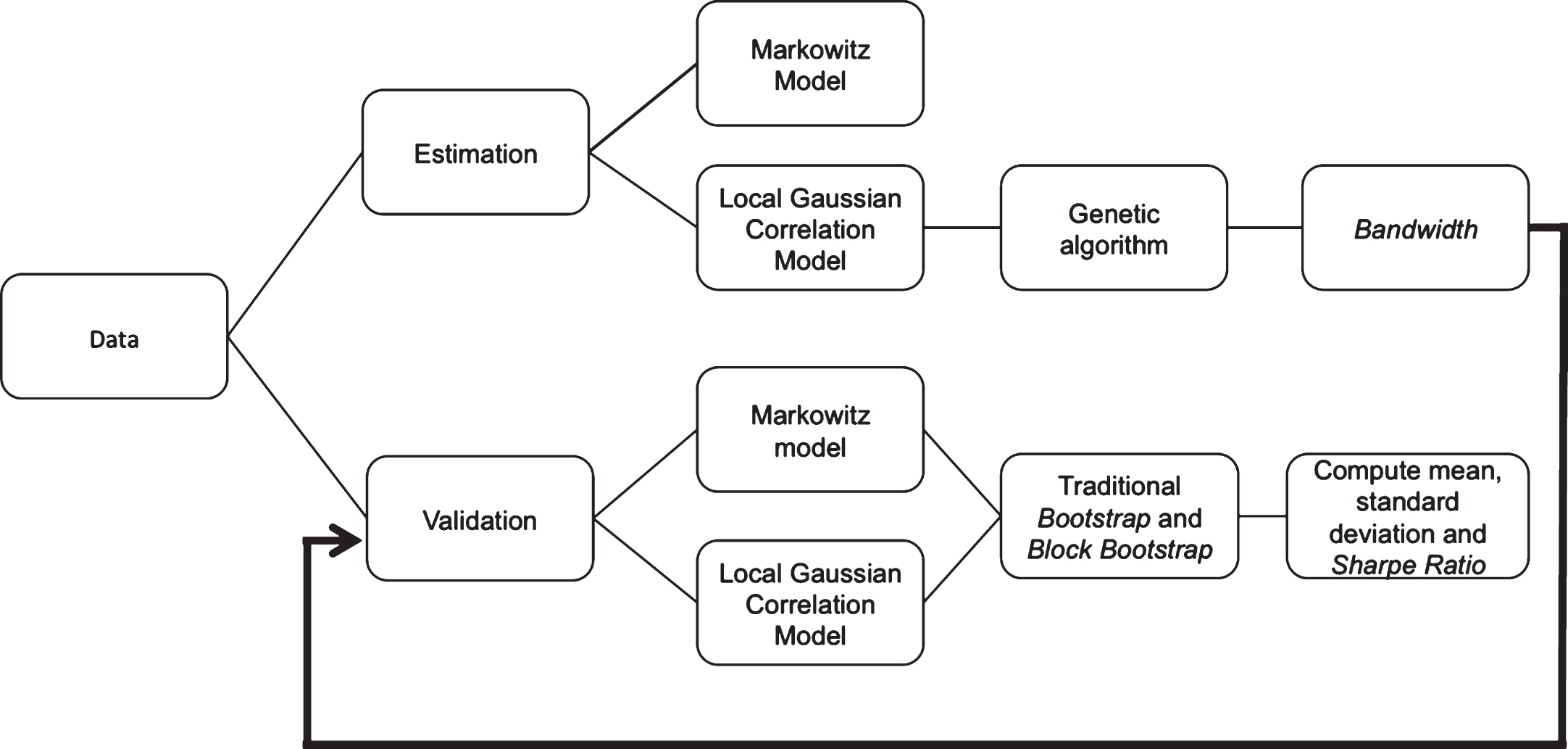
Figure 1 briefly points out the methodology process developed with the financial data.
Fig.1
Methodology using financial data.
Tables 2 and 3 show the results obtained with the application of simple return on ten stocks from S&P500 from 1992 to 2015. The first column reports each year under review, the second name three measures: mean, standard deviation and Sharpe ratio. The third and fourth show the results found using traditional bootstrap in Markowitz (1952) model and in the local Gaussian correlation model, respectively. The fifth and sixth, the results obtained using the block bootstrap in Markowitz (1952) model and in local Gaussian correlation model, respectively. The best result for each year is highlighted in bold.
Table 2
Portfolio results using S&P500 data from 1992 to 2003
| Year | Measure | Markowitz | Local Gaussian | Markowitz | Local Gaussian |
| Bootstrap | Correlation | Block Bootstrap | Correlation Block | ||
| Bootstrap | Bootstrap | ||||
| 1992 | Mean Ret | 0.00091 | 0.00087 | 0.00110 | 0.00096 |
| SD Ret | 0.00077 | 0.00039 | 0.00077 | 0.00037 | |
| Sharpe Ratio | 1.18054 | 2.24235 | 1.42148 | 2.56443 | |
| 1993 | Mean Ret | 0.00048 | 0.00048 | 0.00066 | 0.00054 |
| SD Ret | 0.00087 | 0.00033 | 0.00086 | 0.00086 | |
| Sharpe Ratio | 0.55625 | 1.45163 | 0.76089 | 1.62560 | |
| 1994 | Mean Ret | 0.00059 | 0.00054 | 0.00068 | 0.00054 |
| SD Ret | 0.00079 | 0.00035 | 0.00077 | 0.00043 | |
| Sharpe Ratio | 0.73880 | 1.53047 | 0.87427 | 1.26499 | |
| 1995 | Mean Ret | 0.00080 | 0.00077 | 0.00080 | 0.00072 |
| SD Ret | 0.00102 | 0.00027 | 0.00108 | 0.00028 | |
| Sharpe Ratio | 0.79145 | 2.91316 | 0.73757 | 2.57980 | |
| 1996 | Mean Ret | 0.00137 | 0.00159 | 0.00159 | 0.00168 |
| SD Ret | 0.00103 | 0.00083 | 0.00111 | 0.00083 | |
| Sharpe Ratio | 1.33410 | 1.91418 | 1.43394 | 2.02518 | |
| 1997 | Mean Ret | – 0.00075 | – 0.00091 | – 0.00111 | – 0.00095 |
| SD Ret | 0.00252 | 0.00433 | 0.00266 | 0.00120 | |
| Sharpe Ratio | – 0.29668 | – 0.21132 | – 0.41835 | – 0.79446 | |
| 1998 | Mean Ret | 0.00179 | 0.00195 | 0.00201 | 0.00198 |
| SD Ret | 0.00164 | 0.00096 | 0.00159 | 0.00054 | |
| Sharpe Ratio | 1.09054 | 2.02347 | 1.26150 | 3.65037 | |
| 1999 | Mean Ret | 0.00148 | 0.00167 | 0.00162 | 0.00168 |
| SD Ret | 0.00126 | 0.00110 | 0.00122 | 0.00054 | |
| Sharpe Ratio | 1.17950 | 1.51530 | 1.32768 | 3.11629 | |
| 2000 | Mean Ret | 0.00127 | 0.00111 | 0.00147 | 0.00106 |
| SD Ret | 0.00109 | 0.00045 | 0.00099 | 0.00046 | |
| Sharpe Ratio | 1.16572 | 2.45846 | 1.48417 | 2.31081 | |
| 2001 | Mean Ret | 0.00150 | 0.00158 | 0.00147 | 0.00155 |
| SD Ret | 0.00093 | 0.00031 | 0.00084 | 0.00042 | |
| Sharpe Ratio | 1.61050 | 5.05790 | 1.74546 | 3.69097 | |
| 2002 | Mean Ret | – 0.00017 | 0.00002 | – 0.00024 | – 0.00047 |
| SD Ret | 0.00136 | 0.01213 | 0.00124 | 0.01342 | |
| Sharpe Ratio | – 0.12781 | 0.00170 | – 0.19312 | – 0.03525 | |
| 2003 | Mean Ret | 0.00139 | 0.00141 | 0.00161 | 0.00141 |
| SD Ret | 0.00068 | 0.00245 | 0.00062 | 0.00129 | |
| Sharpe Ratio | 2.04495 | 0.57507 | 2.61074 | 1.09152 |
Table 3
Portfolio results using S&P500 data from 2004 to 2015.
| Year | Measure | Markowitz | Local Gaussian | Markowitz | Local Gaussian |
| Bootstrap | Correlation | Block Bootstrap | Correlation Block | ||
| Bootstrap | Bootstrap | ||||
| 2004 | Mean Ret | 0.00091 | 0.00087 | 0.00110 | 0.00096 |
| SD Ret | 0.00100 | 0.00539 | 0.00094 | 0.00138 | |
| Sharpe Ratio | 1.71612 | 0.32522 | 2.05144 | 1.21543 | |
| 2005 | Mean Ret | 0.00038 | 0.00063 | 0.00035 | 0.00071 |
| SD Ret | 0.00088 | 0.00052 | 0.00097 | 0.00258 | |
| Sharpe Ratio | 0.43537 | 1.22743 | 0.35859 | 0.27743 | |
| 2006 | Mean Ret | 0.00080 | 0.00086 | 0.00075 | 0.00085 |
| SD Ret | 0.00065 | 0.00074 | 0.00066 | 0.00145 | |
| Sharpe Ratio | 1.23416 | 1.16181 | 1.12284 | 0.58959 | |
| 2007 | Mean Ret | 0.00059 | 0.00110 | 0.00085 | 0.00098 |
| SD Ret | 0.00125 | 0.02317 | 0.00141 | 0.01127 | |
| Sharpe Ratio | 0.47186 | 0.04761 | 0.60472 | 0.08719 | |
| 2008 | Mean Ret | – 0.00170 | – 0.00125 | – 0.00253 | – 0.00158 |
| SD Ret | 0.00295 | 0.00139 | 0.00267 | 0.00121 | |
| Sharpe Ratio | – 0.57571 | – 0.90032 | – 0.94733 | – 1.30759 | |
| 2009 | Mean Ret | 0.00182 | 0.00178 | 0.00175 | 0.00180 |
| SD Ret | 0.00087 | 0.00065 | 0.00085 | 0.00182 | |
| Sharpe Ratio | 2.09290 | 2.75062 | 2.05147 | 0.98735 | |
| 2010 | Mean Ret | – 0.00042 | – 0.00043 | – 0.00064 | – 0.00058 |
| SD Ret | 0.00089 | 0.00068 | 0.00092 | 0.00073 | |
| Sharpe Ratio | – 0.47361 | – 0.63353 | – 0.69687 | – 0.78958 | |
| 2011 | Mean Ret | 0.00045 | 0.00057 | 0.00057 | 0.00053 |
| SD Ret | 0.00104 | 0.00077 | 0.00108 | 0.00032 | |
| Sharpe Ratio | 0.43450 | 0.74859 | 0.53223 | 1.63726 | |
| 2012 | Mean Ret | 0.00066 | 0.00078 | 0.00037 | 0.00065 |
| SD Ret | 0.00087 | 0.00269 | 0.00078 | 0.00033 | |
| Sharpe Ratio | 0.75544 | 0.29090 | 0.46580 | 1.95866 | |
| 2013 | Mean Ret | 0.00075 | 0.00080 | 0.00088 | 0.00089 |
| SD Ret | 0.00091 | 0.00046 | 0.00083 | 0.00055 | |
| Sharpe Ratio | 0.82336 | 1.73189 | 1.07122 | 1.63093 | |
| 2014 | Mean Ret | 0.00183 | 0.00137 | 0.00202 | 0.00138 |
| SD Ret | 0.00103 | 0.00010 | 0.00109 | 0.00010 | |
| Sharpe Ratio | 1.77263 | 13.11725 | 1.84394 | 13.86504 | |
| 2015 | Mean Ret | – 0.00194 | – 0.00280 | – 0.00154 | – 0.00234 |
| SD Ret | 0.00280 | 0.03351 | 0.00286 | 0.03836 | |
| Sharpe Ratio | – 0.69321 | – 0.08358 | – 0.53723 | – 0.06112 |
Another way to visualize the results is presented in Figures 2, 3, 4 and 5. It is also possible to obtain an analysis of averages and standard deviations of different methods per year in these following Figures.
Fig.2
Comparing different methods based on return and risk from 1992 to 1997. MB = Markowitz Bootstrap; LGB = Local Gaussian Correlation Bootstrap; MBB = Markowitz Block Bootstrap; LGBB = Local Gaussian Correlation Block Bootstrap.
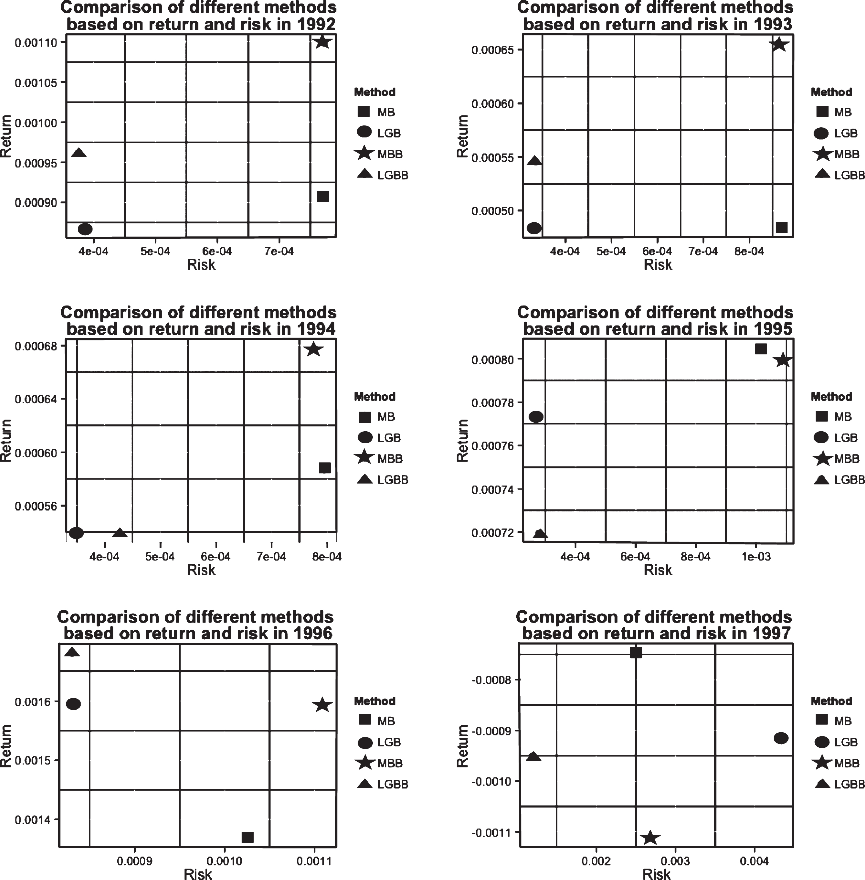
Fig.3
Comparing different methods based on return and risk from 1998 to 2003. MB = Markowitz Bootstrap; LGB = Local Gaussian Correlation Bootstrap; MBB = Markowitz Block Bootstrap; LGBB = Local Gaussian Correlation Block Bootstrap.
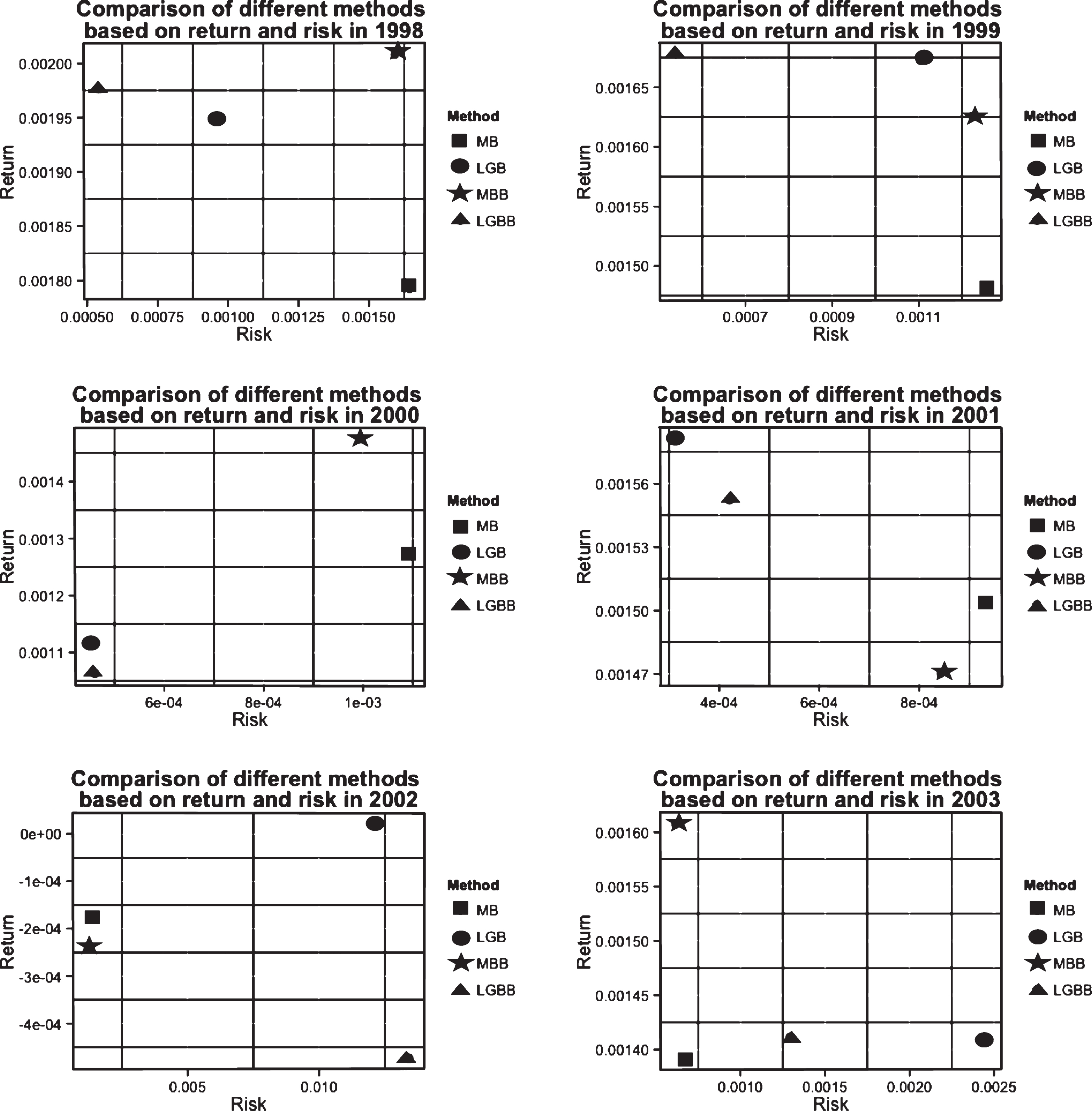
Fig.4
Comparing different methods based on return and risk from 2004 to 2009. MB = Markowitz Bootstrap; LGB = Local Gaussian Correlation Bootstrap; MBB = Markowitz Block Bootstrap; LGBB = Local Gaussian Correlation Block Bootstrap.
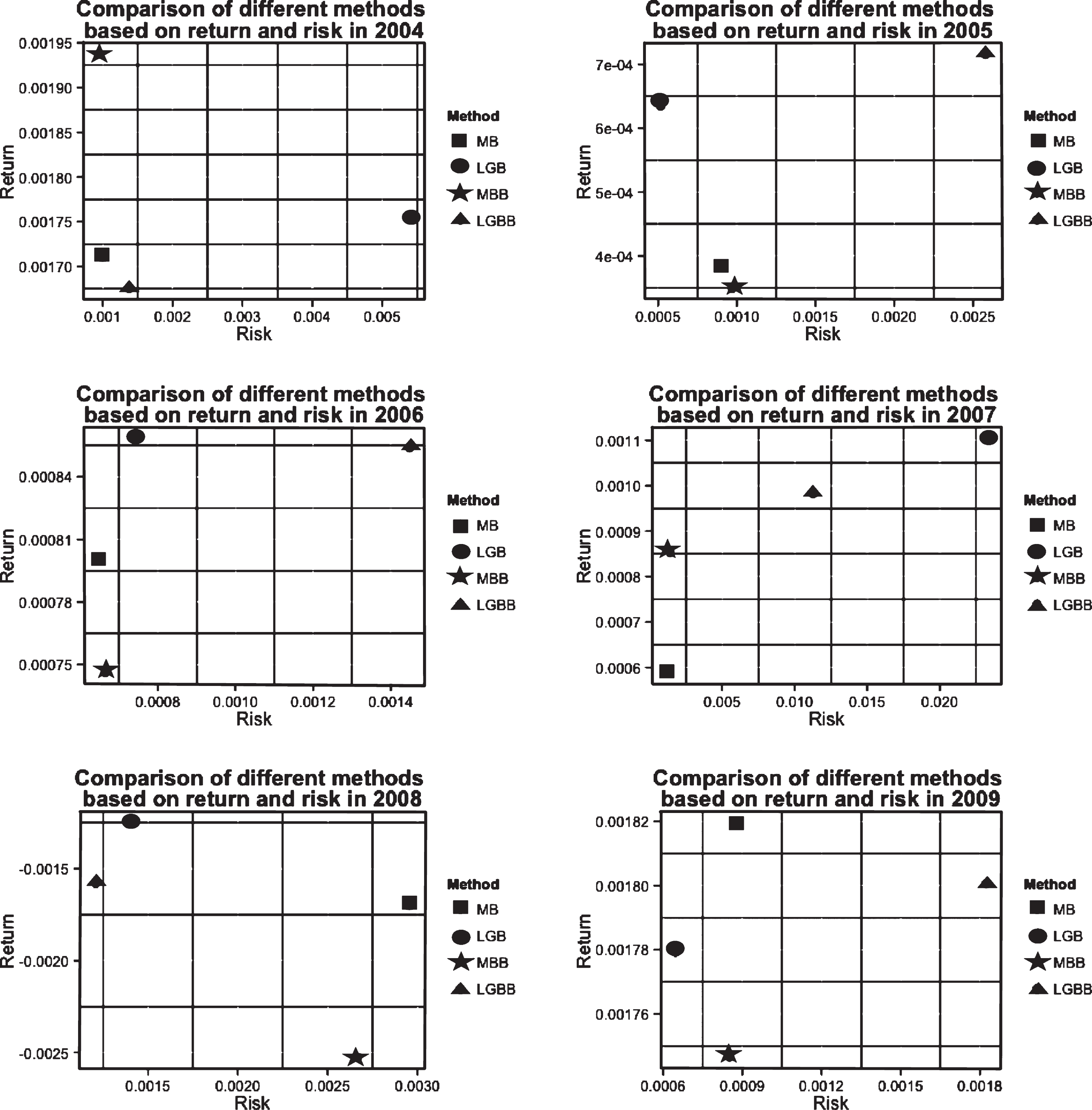
Fig.5
Comparing different methods based on return and risk from 2010 to 2015. MB = Markowitz Bootstrap; LGB = Local Gaussian Correlation Bootstrap; MBB = Markowitz Block Bootstrap; LGBB = Local Gaussian Correlation Block Bootstrap.
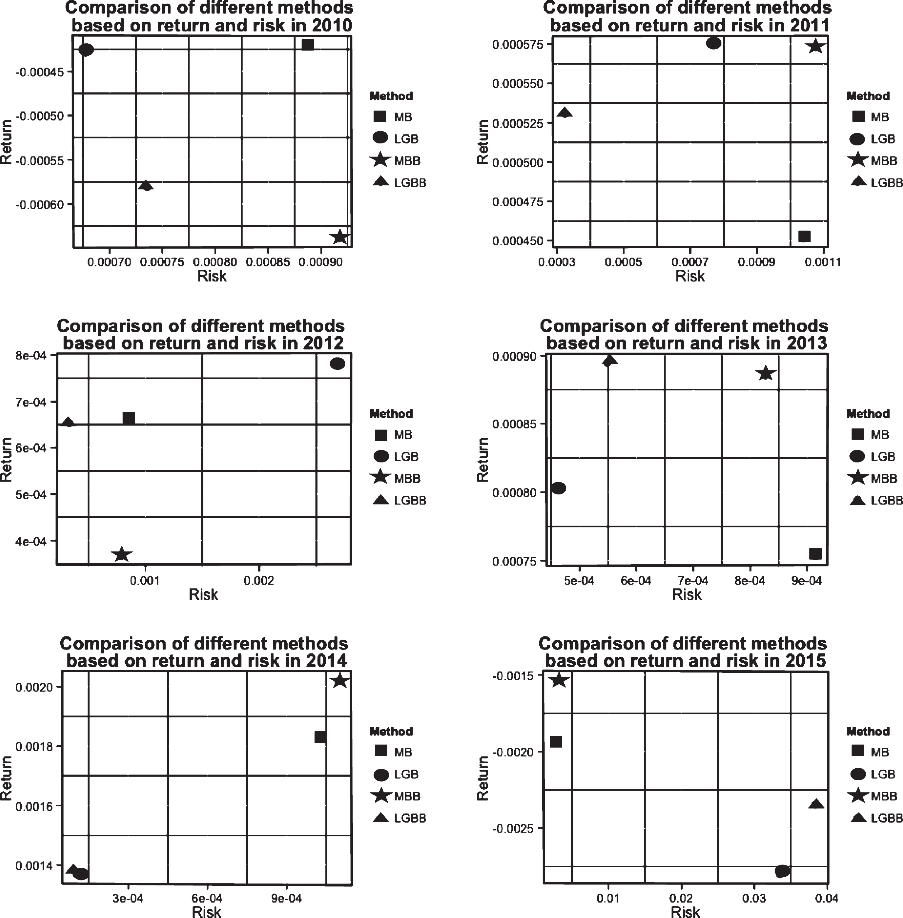
The result analysis shows that the local Gaussian correlation method obtained positive results in the optimal portfolio selection: in 63% of the cases using block bootstrap and in 71% of the cases using the traditional bootstrap. Having presented higher Sharpe ratio, the model generated a more attractive risk-adjusted return.
In other words, we get a higher return of the portfolio compared to its variance as the Sharpe ratio increases. However, combining a high return with low Sharpe ratio implies that the returns were achieved with high risk, which could indicate volatility of returns in the future. It should be noted that past performance does not guarantee what will happen in the future as well as the correlations between securities may undergo rapid change.
In addition, the model that uses local Gaussian correlation did not overcome the Markowitz (1952) model in 1997 due to the Asian financial crisis, in the period of 2003 to 2010 probably because of the financial crisis and in 2010 because of the Flash Crash. Another possible reason of this performance is that the data was divided into 80% for estimation and 20% for validation. As these crises led to a fall in the market, especially at the end of the year, the Sharpe ratio of the local Gaussian correlation was lower. It is important to note that in financial market it is common to observe volatility, however, extreme volatility is undesirable.
5Conclusion
Markowitz (1952) suggested that, for a given fixed number of assets, when the correlation between assets is equal to zero, an investor should diversify among assets according to his interest. However, Casella and Berger (2002) showed that zero correlation does not necessarily imply independence. Thus, it would not be accurate to assume that there is no relationship between those assets, given that the correlation is equal to zero.
Tjøstheim and Hufthammer (2013) pointed out the common view among financial and econometric analysts, that correlation between financial objects becomes stronger as the market declines. Moreover, the correlation value gets close to one with a market crash, resulting in the destruction of the benefit of diversification. Studies indicate the existence of asymmetric dependence between financial returns.
In order to study such asymmetry and overcome these limitations, the local Gaussian correlation model, proposed by Tjøstheim and Hufthammer (2013) presents a new measure of local dependency. According to the authors, the Gaussian distribution provides good approximation in each point of the return distribution. In other words, given an arbitrary distribution, the local Gaussian correlation will seek to find the correlation by adjusting a normal distribution locally. The local correlation in a neighborhood is considered as the correlation of an approximately Gaussian distribution.
Furthermore, the local Gaussian correlation method presents the following advantages: it does not have the conditional correlation bias problem and it is able to detect, in dependence structures, complex or nonlinear changes, which could have been previously masked with global correlation. In this sense, the method provides a better understanding of market dependence (Støve et al., 2014).
In order to improve the model proposed by Markowitz (1952), this paper proposed a modified Markowitz (1952) portfolio allocation that includes two new features: the non-linearity of returns and the non-stationarity of asset returns over time. The technique used to do so was the local Gaussian correlation.
The optimal portfolio estimation using the model proposed here, showed that the group of assets from the S&P500 from 1992 to 2015 obtained a superior performance in 63% of cases using the block bootstrap and in 71% of cases using the traditional bootstrap.
This performance enables managers, financiers and companies to perform a more precise investment analysis. More information regarding the details of the matrix of variance and covariance and the principle of diversification were incorporated into the decision-making process, thus allowing a new way of constructing an optimal portfolio for each investor.
The model also enables the investor to balance the risk and return of the portfolio, as well as indicates how to manage them. That is, the risk can be shared and balanced as a way to mitigate it, allowing managers to adopt more appropriate strategic decisions. An efficient portfolio management aligns the strategic objectives with the organization’s investments.
In the present study, we used 80% of the data from one year for estimation and the remaining 20% for validation. However, the market undergoes several changes in the last few months of the year, as the closing of the balance sheet of many companies and the increase in assets volatility. Thus, it is recommended to use the application of all the data from one year for estimation and the first three months of next year for validation. Instead of estimating the variances and covariance matrix only with past data, it is suggested to incorporate other mechanisms and variables in the matrix, in a way that may affect it over time. The matrix is influenced by the macro-economic context, by the period of time, and by other hidden relations.
References
1 | Ang A. , Chen J. , (2002) . Asymmetric correlations of equity portfolios, Journal of financial Economics 63: (3), 443–494. |
2 | Ardia D. , Boudt K. , Carl P. , Mullen K.M. , Peterson B.G. , (2011) . Differential evolution with deoptim, The R Journal 3: (1), 27–34. |
3 | Bachelier L. , (1900) . Théorie de la spéculation. Gauthier-Villars. |
4 | Bampinas G. , Panagiotidis T. , et al., (2017) . Oil and stock markets before and after financial crises: a local gaussian correlation approach. Technical report, Bank of Estonia |
5 | Berentsen G.D. , Tjøstheim D. , (2014) . Recognizing and visualizing departures from independence in bivariate data using local gaussian correlation, Statistics and Computing 24: (5), 785–801. |
6 | Campbell J.Y. , Lo A.W.-C. , MacKinlay A.C. , et al., (1997) . The econometrics of financial markets, volume 2: , princeton University press Princeton, NJ. |
7 | Campbell R.A. , Forbes C.S. , Koedijk K.G. , Kofman P. , (2008) . Increasing correlations or just fat tails? Journal of Empirical Finance 15: (2), 287–309. |
8 | Casella G. , Berger R.L. , (2002) . Statistical inference, volume 2: . Duxbury Pacific Grove, CA. |
9 | Chollete L. , Heinen A. , Valdesogo A. , (2009) . Modeling international financial returns with a multivariate regime-switching copula, Journal of Financial Econometrics nbp014. |
10 | Cont R. , (2001) . Empirical properties of asset returns: stylized facts and statistical issues. |
11 | Dietterich T.G. , (2000) . Ensemble methods in machine learning. In International workshop on multiple classifier systems, pp. 1–15. Springer. |
12 | Efron B. , (1992) . Bootstrap methods: another look at the jackknife. In Breakthroughs in Statistics, pp. 569–593. Springer. |
13 | Fama E.F. , (1998) . Market effciency, long-term returns, and behavioral finance, Journal of Financial Economics 49: (3), 283–306. |
14 | Garcia R. , Tsafack G. , (2011) . Dependence structure and extreme comovements in international equity and bond markets, Journal of Banking & Finance 35: (8), 1954–1970. |
15 | Goldfarb D. , Iyengar G. , (2003) . Robust portfolio selection problems, Mathematics of Operations Research 28: (1), 1–38. |
16 | Hjort N.L. , Jones M. , (1996) . Locally parametric nonparametric density estimation, The Annals of Statistics, pp. 1619–1647. |
17 | Hong Y. , Tu J. , Zhou G. , (2007) . Asymmetries in stock returns: statistical tests and economic evaluation, Review of Financial Studies 20: (5), 1547–1581. |
18 | Horst U. , Rothe C. , (2008) . Queuing, social interactions, and the microstructure of financial markets, Macroeconomic Dynamics 12: (02), 211–233. |
19 | Huang Z. , Victor H. , Chollete L. , (2014) . Local dependence: A bird’s-eye view of dependence in different quadrants. Texto de discusso. |
20 | Hudson R.S. , Gregoriou A. , (2015) . Calculating and comparing security returns is harder than you think: A comparison between logarithmic and simple returns, International Review of Financial Analysis 38: , 151–162. |
21 | Inci A.C. , Li H.-C. , McCarthy J. , (2011) . Financial contagion: A local correlation analysis, Research in International Business and Finance 25: (1), 11–25. |
22 | Kendall M.G. , Hill A.B. , (1953) . The analysis of economic time-series-part i: Prices, Journal of the Royal Statistical Society. Series A (General) 116: (1), 11–34. |
23 | Lura A. , (2013) . The norwegian stock market:-a local gaussian perspective. |
24 | Mandelbrot B.B. , (1997) . The variation of certain speculative prices. Springer. |
25 | Markowitz H. , (1952) . Portfolio selection, The Journal of Finance 7: (1), 77–91. |
26 | Markowitz H. , (1959) . Portfolio Selection, Effcent Diversification of Investments. J. Wiley. |
27 | Meucci A. , (2010) . Quant nugget 2: Linear vs. compounded returns-common pitfalls in portfolio management. GARP Risk Professional, pp. 49–51. |
28 | Okimoto T. , (2008) . New evidence of asymmetric dependence structures in international equity markets, Journal of Financial and Quantitative Analysis 43: (03), 787–815. |
29 | Otneim H. , Tjøstheim D. , (2017) . Conditional density estimation using the local gaussian correlation. Statistics and Computing, pp. 1–19. |
30 | Patton A.J. , (2004) . On the out-of-sample importance of skewness and asymmetric dependence for asset allocation, Journal of Financial Econometrics 2: (1), 130–168. |
31 | Politis D.N. , White H. , (2004) . Automatic block-length selection for the dependent bootstrap, Econometric Reviews 23: (1), 53–70. |
32 | Rodriguez J.C. , (2007) . Measuring financial contagion: A copula approach, Journal of Empirical Finance 14: (3), 401–423. |
33 | Silvapulle P. , Granger C.W., (2001) . Large returns, conditional correlation and portfolio diversification: a value-at-risk approach. |
34 | Statman M. , (1987) . How many stocks make a diversified portfolio? Journal of Financial and Quan-Titative Analysis 22: (03), 353–363. |
35 | Støve B. , Tjøstheim D. , (2013) . Measuring asymmetries in financial returns: An empirical investigation using local gaussian correlation. |
36 | Støve B. , Tjøstheim D. , Hufthammer K.O. , (2014) . Using local gaussian correlation in a nonlinear re-examination of financial contagion, Journal of Empirical Finance 25: , 62–82. |
37 | Tjøstheim D. , Hufthammer K.O. , (2013) . Local gaussian correlation: a new measure of dependence, Journal of Econometrics 172: (1), 33–48. |
38 | Working H. , (1934) . A random-difference series for use in the analysis of time series, Journal of the American Statistical Association 29: (185), 11–24. |

