
Study of the periodicity in Euro-US Dollar exchange rates using local alignment and random matrices
Abstract
The purpose of this study was to detect latent periodicity in the presence of deletions or insertions in the analyzed data, when the points of deletions or insertions are unknown. A mathematical method was developed to search for periodicity in the numerical series, using dynamic programming and random matrices. The developed method was applied to search for periodicity in the Euro/Dollar (Eu/$) exchange rate. The presence of periodicity within the period length equal to 24 hours and 25 hours, in the analyzed financial series, was shown. Periodicity can be detected only with insertions and deletions. The results of this study show that periodicity phase shifts, depend on the observation time. A period of 24 hours is a common phenomenon for foreign exchange rates, indices and stocks of different companies. We show it for the Bank of America and Microsoft stocks, S&P500 and NASDAG indexes and for the gold and silver prices as examples. The reasons for the existence of the periodicity in the financial ranks are discussed. The results can find application in computer systems, for the purpose of forecasting exchange rates.
Identification of the cyclic patterns in numeric time series and symbolical sequences may shed light on the processes occurring in systems of a different nature and give information about the structure of different time series. Currently, there are many mathematical methods for studying symbolic sequence periodicity. This is due to the necessity of studying DNA sequences and amino acid sequences of proteins (Miller, 2006; Mount, 2004). To identify periodicities in the time series and symbolical sequences, the methods mainly used are based on the Fourier transform, wavelet transform and dynamic programming, as well as some other method (Benson, 1999; Chechetkin and Turygin AYu, 1995; Coward and Drabløs, 1998; Dodin et al., 2000; Fadiel et al., 2006; Granger and M, 1967; Hamilton, 1994; Jackson et al., 2000; Makeev and Tumanyan, 1996; Marple, 1987; Oppenheim et al., 1999; Rackovsky, 1998; Stankovic et al., 2005; Stoica P and Moses R, 2005; Struzik, 2001). Previously, we proposed the method of informational decomposition, which allows the detection of periodicity in both symbolic and numeric sequences; however, the detection was severely impeded by the above approaches (Korotkov et al., 2003). These difficulties emanate from the fact that methods based on Fourier and Wavelet transform, decompose the statistical significance of long periods (larger than the size of the analyzed sequence alphabet) for smaller periods with a multiple of the length (Korotkov et al., 2003). Also, these methods are very sensitive to the insertion and deletion of symbols. This leads to the fact that spectral methods cannot detect periodicity at a statistically significant level, even in the presence of a few deletions or insertions. Dynamic programming, which allows the detection of deletions and insertions in the periods, cannot detect relatively “fuzzy” periodicity. This is due to the fact that this method is based on finding the similarity between pairs of periods in the studied sequence (Benson, 1999). However, if a statistically significant similarity is absent between two separate periods, dynamic programming will fail to detect periodicity in the analyzed sequence. The lack of similarity between two separate periods can be observed for latent periodicity, where the periodicity occurs on the background of random noise (Korotkov et al., 2003). To find such periodicity, the method of informational decomposition was used (Korotkov et al., 2003). This method enabled the discovery of latent periodicity in the DNA sequences of many genes (Chaley et al.,1999; Korotkov et al., 1997) and revealed the latency of amino acid specific for the protein families (Korotkov et al., 1999; Turutina et al., 2006). These results suggest that latent periodicity with insertions and deletions can be detected in sequences of a different nature and in numerical sequences also.
Today, it is known that people, animals and plants have biological rhythms. The manifestation of these rhythms can be observed at all levels of biological organization. The interaction can be observed between the rhythms that affect the internal state of the person and on various social processes. A. Chizhevsky (1976) first drew attention to the influence of natural factors on social processes The biological rhythms can also influence currency rates. If the periods in the exchange rates exist, then the various events in public life can affect them. Such events can lead to changes in the data and could be identified as a phase shift of the period. The phase shifts in the sequence could have resulted from deletion or insertion of values with respect to the existing period. Therefore, in order to detect this periodicity, it was necessary to develop a mathematical method for detecting the periodicity of the time series, taking into account the unknown location and unknown number of insertions or deletions, in the presence of large noise. It cannot be done with the help of all known mathematical methods. Previous studies have searched for insertions or deletions (Rastogi et al., 2006), but failed to find a periodicity with large noise (Suvorova et al., 2014). It is right mainly for dynamic programming. Either of these methods works well in the presence of large noise, but fails to find periodicity in the presence of even small amounts of insertions and deletions (Korotkov et al., 2003).
This paper contributed to filling the gap in mathematical methods for periodicity search. A mathematical method was developed to find periodicity in the symbolical sequences, in the presence of insertions and deletions and the big noise. The method was developed using the random matrices of periodicity and the method of dynamic programming. The developed method was applied to search for periodicity in the exchange rate of the Euro to the US Dollar. To search for periodicity, the numerical sequence was converted to a symbolical sequence. The calculations show that there is a periodicity equal to 24 and 25 h in the Euro-Dollar exchange rate. This periodicity of the exchange rate contains a lot of insertions and deletions and could not be detected by previously developed mathematical methods. The periodicity with 24 hour period is observed in a stock, financial indexes and prices. We show here the periodicity the Bank of America and Microsoft stock, S&P500 and NASDAG indexes and the gold and silver prices as examples.
1Methods and algorithms
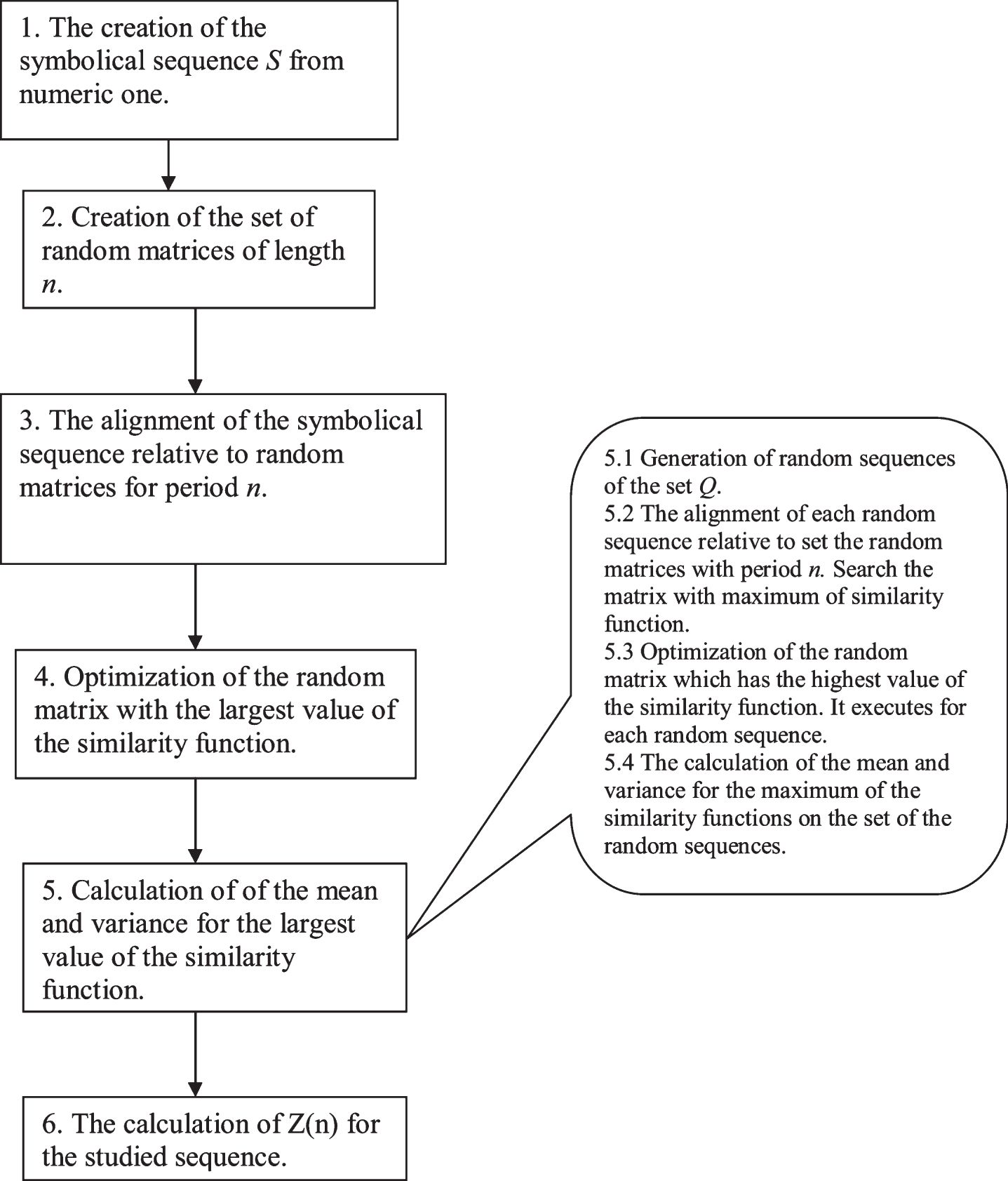
To search the periodicity with insertions and deletions, the algorithm shown in Fig. 1 was used. As can be seen from the algorithm, firstly, a set of random matrices (Fig. 1, paragraph 2) with size 20xn was generated, where n is the length of the period, and 20 is the alphabet size of the studied sequence. Then, a local alignment of the studied sequence was built relative to each of the generated random matrices (Fig. 1, paragraph 3). Dynamic programming was used to build the local alignment and in determining the similarity function F. Then, the matrices were transformed because the distribution of the similarity function F maximum for each of the matrices for the set of all random sequences (set Q, paragraph 2.2) should be similar. The transformed matrix having the highest value of the similarity function F, with the studied sequence S, was chosen. Then, this matrix was optimized to achieve the highest value of the similarity function F (maxF) with the studied sequence S (Fig. 1, paragraph 4) and the transformed matrix was called T. Then, the value of maxF for each random sequence from the set Q and for matrix T was calculated. It allowed the mean value and variance for maxF to be determined (Fig. 1, paragraphs 5.1–5.4). This algorithm was applied for periods of different lengths and for each length of the period n, the corresponding value of Z was calculated (formula 7). As a result of the algorithm, the dependence of Z on n was obtained and denoted as Z(n). (Fig. 1, paragraphs 6). It should be noted that in this study, dynamic programming was used to find a local alignment. This means that the boundaries of the regions with maxF, may differ from the beginning and end of the studied sequence. It means also that the values of Z(n) for different n can be obtained for different fragments of the studied sequence. The boundaries of the fragments, obtained for relevant values of Z(n) are shown. Subsequently, each step of the algorithm shown in Fig. 1 was examined in more detail.
Fig.1
Scheme of the mathematical algorithm which was used to calculate the statistical significance of period Z of length n in the studied sequence.
1.1Creation of a character sequence from a numerical sequence
The candle opening and closing was separated by an interval of 1 h. Let x1(i) –be the rate at the time of opening of the candle, and x2(i)- the rate at the close of the candle. The sequence A, we calculated the difference s(i) = x2(i)-x1(i), where x1(i) and x2(i) are separated by hour. The numeric sequence A of length N was transformed in the symbolic sequence S with alphabet of 20 letters (Fig. 1, paragraph 1). To convert the numerical sequence, the minimum and maximum elements of the sequence A were determined. Then, this interval was divided into 20 intervals, the number of elements of the numeric sequence in each interval was approximately equal to N/20. Each interval received the letter of the Latin alphabet. If a numeric sequence contained many of the equal values than the boundaries of the intervals were varied in such a way that the same numbers were encoded by the same symbol. We created the sequences S for Euro/Dollar (Eu/$) exchange rate (sequence S1) Bank of America (sequence S2) and Microsoft stock (sequence S3), S&P500 (sequence S4) and NASDAG (sequence S5) indexes and the gold (sequence S6) and silver (sequence S7) prices. The sequence S1 encoding is shown in Table 1. The sequence S1 was obtained for data from 01.03.2016 to 20.12.2016. Sequences S6 and S7 were received from 01.03.2016 to 20.12.2016. The sequences S2, S3, S5, S5 were obtained for data from 01.03.2016 to 20.12.2016. Method can analyze the sequence no longer than 5000 symbols and it determines the time interval for analysis. Numerical data were taken from the site http://finam.ru, Moscow time.
Table 1
The coding of sequence A2 to obtain the sequence S1 is shown
| K | N | I | M | T | R | S | L | Y | F |
| –0.00880– | –0.00120– | –0.00080– | –0.00060– | –0.00040– | –0.00030– | –0.00020– | 0.00020– | –0.00010 | 0.00000 |
| 0.00120 | 0.00080 | 0.00060 | 0.00040 | 0.00030 | 0.00020 | 0.00020 | 0.00010 | 0.00000 | 0.00000 |
| C | W | P | H | Q | V | A | D | E | G |
| 0.00000 | 0.00010 | 0.00010 | 0.00020 | 0.00020 | 0.00030 | 0.00040 | 0.00060 | 0.00080 | 0.00110 |
| 0.00010 | 0.00010 | 0.00020 | 0.00020 | 0.00030 | 0.00040 | 0.00060 | 0.00080 | 0.00110 | 0.00100 |
We also used the candle separated by an interval of 0.5 h and 4 h for Euro/Dollar (Eu/$) exchange rate and we generated the sequences S8 and S9. These sequences contain 4800 symbols and data of last kindle is 20.12.2016.
1.2Generation of random sequences
A set Q of random sequences was created by random shuffling of the sequence S (Fig. 1, Paragraph 5.1) and the set Q containing 200 sequences. To generate one random symbolical sequence, a random number sequence of length N was generated by the random number generator. Then, a random number sequence was arranged in ascending order, storing the generated permutations. The produced permutations were used for mixing the sequence S, and as a result of this mixing the random symbolic sequence from the set Q was created.
1.3Creation of a set of random matrices with length n
Random matrices with the dimension 20xn were used, where n is the length of the period (Fig. 1, Paragraph 2). Each matrix can be viewed as a point in space 20xn. A set of random matrices W was created when the distance between them in the space 20xn should not be less than a certain value. To calculate the differences between the two matrices m1(i,j) and m2(i,j), the information measure was used (Kullback, 1997):
(1)
where
(2)
Hence, 2I (M1, M2) has an approximately χ 2 (df) and df equal to 19n because I1 (M1, M2), I2 (M1, M2),..., In-1 (M1, M2) are independent and In (M1, M2) is completely determined by I1 (M1, M2), I2 (M1, M2),..., In-1 (M1, M2)(Kullback, 1997). Then we used the approximation of the chi-square distribution by the normal distribution:
(3)
The value x (M1, M2) ∼ N (0, 1)  N(0,1) was obtained and is an argument of the standard normal distribution. N(0,1) is very useful as a measure of the differences between the matrices m1(i,j) and m2(i,j). The probability p = P(x > x(M1,M2)) shows that the differences between the matrices m1(i,j) and m2(i,j) are determined by random factors. If the difference between the matrices m1(i,j) and m2(i,j) increases, then N(0,1) becomes larger. The difference between matrices not less than 1.0 was chosen.
The used algorithm to generate matrices was next. Each element of the matrix m(i,j), i = 1,...,20, j = 1,...,n was randomly filled with equal probability either 0 or 1. Then, the matrix was compared with all matrices, which were already included in the set W. If at least one matrix has this difference, less than L = 1.0, then the generated matrix was not included in the set W. If the difference was greater than L = 1.0 for all matrices from the set W, then the matrix is included in the set W. The 108 of such matrices were created for each period length n. These matrices were used to construct the alignments for sequences created in paragraph 2.1.
1.4Alignment sequence S relative to the random matrices
To search for the periodicity in the sequence S with insertions and deletions, an alignment sequence S relative to the modified matrices m’ from the W set was performed; a method of modifying matrices is described below (Fig. 1, paragraph 3). To build alignment, the matrix for the similarity function F was filled, using a modified matrix m’(i,j).
(4)
where s(i) –element of the sequence S, d –weight per insertion or deletion of a symbol in the sequence S. Here, i and j changed from 1 to n; k = j –n*int((j-0.1)/n). This means that the index j always corresponds to the column of the matrix k. The matrix F has dimension N by N, where N is the length of the sequence S. Simultaneously, with the filling of the matrix of the similarity function F, the matrix of inverse transitions F’ was filled. It has the same dimension as the matrix F. Each element of the matrix F’(i,j) contains the number of the element of the matrix F, for which the maximum is reached in the formula (4). After filling in the matrices F and F’, the maximum element maxF in the matrix F and its coordinates (im, jm) were determined. The alignment of the sequence S concerning the sequence of indices k was created with help of the matrix of the inverse transitions F’, as earlier described (Polyanovsky et al., 2011). The path in the matrix F from the point (im, jm) to the point (i0, j0) corresponds to the created alignment. At the point (i0, j0), the function F became equal to zero for the first time and served as the beginning of the alignment. The first sequence of the alignment is the sequence of numbers k, and the sequence S is the second sequence in the alignment. Each column k in the alignment, mapped the symbol of the sequence S, or sign * which indicates that this column is not mapped to any symbol of the sequence S. Similarly, each symbol of the sequence S is associated with a specific column k or sign * which indicates that this symbol is not mapped to any column k. To build the alignments created in paragraph 2.1 and 2.2 sequences, the modified matrix m’ from the set W was used. Firstly, the values A and B for matrix m were calculated as:
(5)
(6)
where p(i) = n(i)/N, n(i) is the number of symbols of type i in the sequence S, N is the total number of symbols in the sequence S.
To carry out the alignment, the matrix m’ needs to satisfy two conditions. The first condition is that the A values for matrix m’ with the same period length n would be the same and equal to 200*n. The second condition is that the distribution functions for maxF would be most similar for all matrices of length n. The distribution for each matrix can be built to align each matrix length n with random sequences from the set Q and to determine the maxF for each sequence from set Q. The value of the constant B for each matrix was selected, which provided maximum identity for the distribution function maxF, for matrices on the set Q with the same n value. The two conditions shown above, allow the replacement of matrix m on the matrix m’, for which these conditions are satisfied. Equation (5) is the equation of the surface of the ball in space 20xn, and Equation (6) is the equation of the plane. If the matrix m’ satisfies these conditions, then it lies on a circle formed by intersection of the surface of the balloon (Equation 5) by the plane (Equation 6). The matrix m is considered as a point in space 20xn, from which the nearest point was obtained, which lies on the circle formed by the intersection of the surface plane with the ball. The coordinates of this point are the m’ matrix. It is easy to write a few simple equations to determine the coordinates of this point (the values of the matrix m’) on base of the matrix m, using Equations 5 and 6. Practically, this means that the constants A, B, and the matrix m can be used to calculate the p(i) for a sequence S, thus the matrix m’ can be clearly defined (if there is an intersection of the surface of the plane with the ball plane). Further, the aim was to find for each matrix length equal n the constant B, which would ensure a maximum identity of the distribution function of maxF on the set of sequences Q.
Simultaneously, with the calculation of the distribution function for maxF on the set of sequences Q, the average length of a random alignment was calculated as the difference (im-i0), where im –is coordinate of the maxF in the sequence S, and i0 –coordinate, where F = 0.0 (the coordinate of the beginning of the alignment in the sequence S). The average length of a random alignment equal to 600±60 symbols was selected. This value provides the best search of the alignment boundaries relative to the real boundaries on the model sequences. The choice of the constant B was carried out by an iterative procedure. The constant B, which gives
1.5Optimization of a random matrix with the largest value of the similarity function
For all matrices from the set W, was determined the modified matrix max(m’) which had the highest value of the similarity function maxF. For it, the alignment was calculated and the coordinates of the alignment were determined (Fig. 1, paragraph 4). However, despite the fact that a very large number of matrices was used, the matrix max(m’) may have the value maxF, which is not the largest for a sequence S and for length of period n. This means that the largest value can be achieved for the matrix T, which lies at some distance from the matrix max(m’) that is less than the chosen threshold L (paragraph 2.3). Therefore, approximately 107 matrices were created, having distance from the matrix max(m’) L less than that specified in paragraph 2.3 (L = 1.0) but greater than 0.0. This means that the difference L with max(m’) matrix was in the range (0.0–1.0). These matrices were also used, as indicated in paragraph 2 and a final matrix T was chosen which had the highest value maxF. The described algorithm is faster than the genetic algorithm used for matrix optimization (Pugacheva V.M. et al., 2016).
1.6Calculation of Z values for the period n of the studied sequence
The procedures described in paragraphs 2.4 and 2.5 were used for random sequences from the set Q. This allowed the mean value
(7)
As a result, the dependence Z(n) for symbolic sequences S (Fig. 1, paragraphs 5-6) was constructed. As sequence S we used the sequences S1–S9.
1.7The using of the Fourier transform and its statistical significance
The results obtained from the study of sequences S1 were compared with the results on a search of periodicity, using the Fourier transform. Fourier transform calculates the intensity of the spectral density for a set of orthogonal periods (Granger & M, 1967). However, for a comparative study of our method with the method of Fourier transform, it is desirable to consider not a spectral intensity but the magnitude similar to the Z(n), defined by formula (5).
To build this spectrum, numeric values of the analyzed sequence were randomly mixed, without changing the values of the sequence. After this mixing, a numerical sequence same length as the original was received, and to this sequence we applied the Fourier transform. A 1000 sequence shuffle was done and the resulting intensity for each orthogonal period had a range of 1000 values. This range allowed the determination of the mean value and variance of intensities for different period lengths. As a result, for each intensity the value of Z was determined by formula (7) and a Fourier transform spectrum identical to the spectra obtained in paragraph 2.6, was obtained.
2Results and discussion
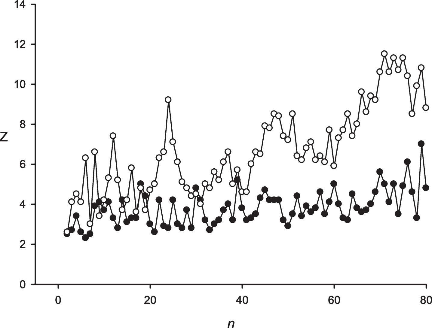
Figure 2 shows the application of the developed approach to the random sequence and the sequence S10 obtained from the sequence S10’ = (EFKLWNMSTWRYLQKLWQSMETMQ)16. In random cases 75% substitutions were performed in the sequence S10’; and after that our developed approach was applied. The results of the random sequences analysis demonstrate that Z(n) fluctuated around 4.0. It should be noted that the insignificant trend toward increasing the Z-values in the random sequence corresponds to the periodicity length of more than 70. Judging from these results, it could be concluded that periodicities with Z-values >7.0 were found to be interesting. The results of the S3 sequence study show that the developed approach could be applied to identify the fuzzy frequency and determine the optimal weighting matrix for the detection of periodicities with the length equal to 24 symbols. It is possible to register the periodicities equal to 48 and 72 symbols. However, significant Z-values also received periodicities with the lengths close to 48 and 72 symbols, because there appears a possibility of insertions or deletions. It is always possible to perform insertions or deletions to align the sequence S3 against the matrices and to receive periodicities close to 48–72 symbols with a high Z-value. However, this leads to a slight drop in the Z-values, which is related to the penalties for insertions or deletions. So, the graph around 48 and 72 symbols looks like a gently sloping mountain.
Fig.2
Black circles show the Z(n) for the random sequence. White circles show the Z(n) for the artificial sequence with a period of 24 symbols with total length of 384 symbols and 75% random substitutions. It is evident that despite the large number of random substitutions, the developed mathematical method could detect the periodicity with n = 24.
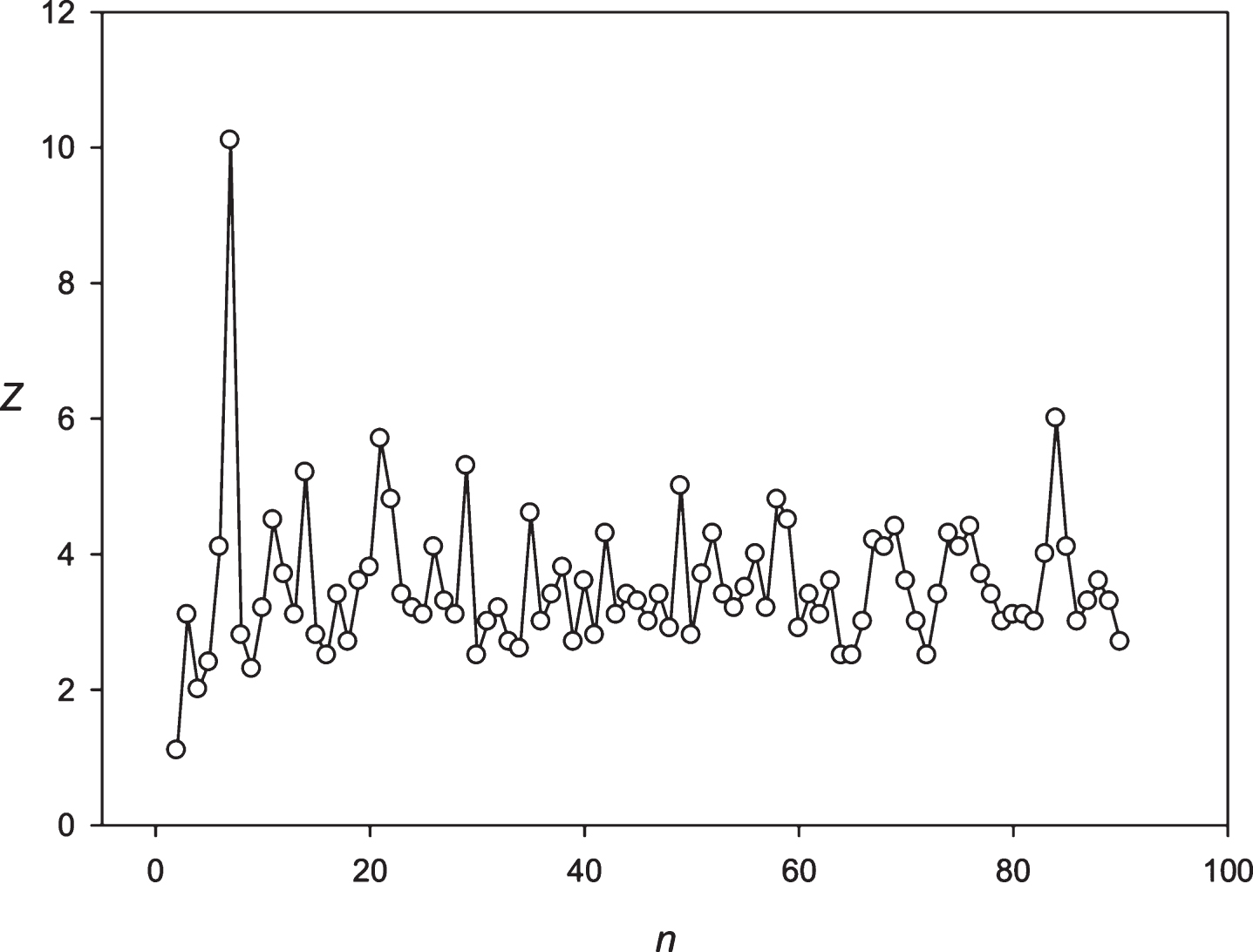
Next, the developed approach was applied to the periodicity search within the symbol sequence S1 (paragraph 2.6). The Z(n) spectrum obtained for the sequence S1 is shown in Fig. 3. For the sequence S1, periodicities were registered in 24 and 25 h. Both periodicities were analyzed based upon almost the same data. The 24 h periodicity was observed for the 29 to 4165 h sequence S1 ; and the 25 h periodicity was observed from the 29 to 4224 h sequence S1. The periodicity equal to 25 h was the mostly statistically expressed (Z≈14.0), compared to the periodicity having the length of 24 h (Z≈10.5). It could be assumed that building a significant alignment for two periodicities is associated with the ability to create symbol insertions or deletions in the sequence S1.
The optimal weighting matrix for the 24 h periodicity is shown in Table 2. This matrix was obtained by applying the developed algorithm. The matrix in Table 2 demonstrates that the matrix elements oscillation amplitude max(m’) is different in different columns. The matrix shows that every hour is characterized by significant fluctuations in up and down directions.
Fig.3
The spectrum of Z(n) obtained for the sequence S1 (paragraph 2.6).
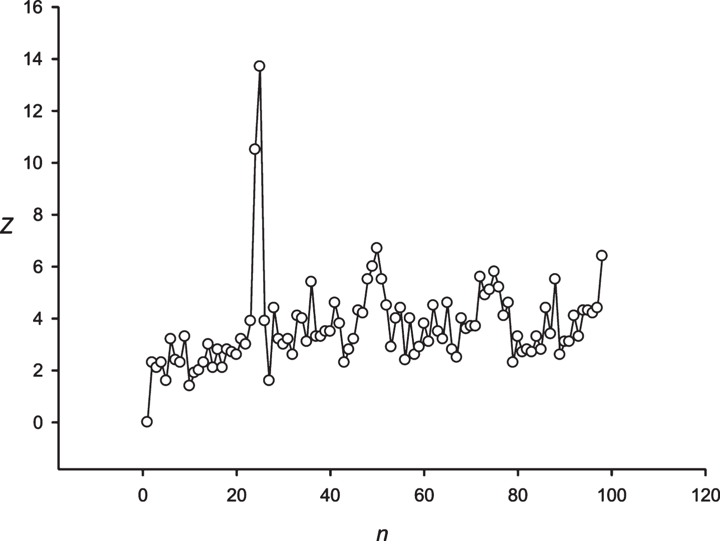
Table 2
The table contains the weight matrix for periods equal to 24 h. Position period and the weight for each symbol in each position of the period are shown
| 1 | 2 | 3 | 4 | 5 | 6 | 7 | 8 | 9 | 10 | 11 | 12 | |
| K | 1.6 | 1.8 | –0.1 | 0.7 | –2.7 | –2.3 | –2.7 | –1.0 | –1.4 | –3.1 | –2.7 | –0.6 |
| N | 2.0 | 1.5 | 1.9 | –0.6 | –1.9 | –1.0 | –2.7 | –3.2 | –3.2 | –1.9 | –3.2 | –0.6 |
| I | 2.2 | –1.8 | 0.3 | 1.5 | 1.5 | –1.8 | –1.0 | –0.1 | –3.1 | –1.8 | –0.5 | –1.0 |
| M | –1.4 | –0.5 | 0.4 | 1.5 | –0.5 | 1.5 | –0.5 | –1.8 | –0.5 | 1.2 | –0.5 | –3.1 |
| T | –3.6 | 1.7 | –1.9 | 1.6 | –0.7 | –1.1 | 1.7 | –1.9 | –0.7 | –0.3 | –1.9 | 0.6 |
| R | –0.1 | –2.3 | 0.3 | 1.2 | 1.5 | 0.3 | 1.5 | –1.4 | –0.1 | 1.9 | –3.1 | –1.0 |
| S | 0.5 | –3.3 | –2.8 | 1.3 | 1.4 | –1.6 | –0.7 | 1.5 | –1.2 | –1.2 | 1.5 | 1.5 |
| L | –1.1 | –0.6 | –3.2 | –0.2 | –0.2 | –1.5 | 0.6 | –0.6 | 1.3 | 1.7 | 1.7 | 1.8 |
| Y | –1.3 | –2.2 | 1.6 | –2.6 | 1.3 | 1.7 | –0.4 | 1.7 | 1.6 | –1.7 | 1.6 | –1.7 |
| F | –2.8 | –1.6 | –0.7 | –2.4 | 1.0 | 1.7 | –0.3 | 2.1 | 1.7 | –0.3 | 1.6 | 1.4 |
| C | –2.3 | –0.5 | –2.3 | –0.5 | 0.3 | –2.3 | 1.2 | 1.6 | 1.8 | 1.8 | 0.8 | 1.7 |
| W | –0.7 | –1.1 | –1.6 | –0.7 | 1.6 | 1.8 | –1.1 | –2.4 | 0.5 | 1.4 | 1.3 | –2.8 |
| P | –1.9 | –1.5 | –0.2 | –1.5 | –3.2 | 0.3 | 1.5 | 1.5 | 1.8 | 0.7 | 1.5 | 1.8 |
| H | –1.1 | –2.4 | –1.5 | –1.9 | 1.6 | 1.6 | 1.7 | 1.7 | 1.3 | 1.7 | –0.3 | –1.5 |
| Q | –1.3 | –1.7 | –0.9 | 0.0 | –2.6 | 1.3 | 0.5 | 1.3 | 1.3 | –2.6 | 1.4 | 0.9 |
| V | –0.5 | –1.0 | –1.0 | 1.4 | 1.2 | 0.3 | 1.8 | –1.4 | –0.1 | 0.7 | 0.7 | 1.5 |
| A | 0.3 | –1.4 | 1.8 | –2.3 | 1.6 | –2.3 | 1.4 | –1.0 | –2.3 | 0.3 | 1.4 | 0.3 |
| D | 1.7 | 1.2 | –1.4 | 1.4 | 0.7 | –0.5 | –1.8 | –1.0 | –1.0 | –1.8 | –2.3 | –0.1 |
| E | –2.3 | 2.2 | 2.1 | –0.6 | –3.2 | –1.0 | –2.7 | –3.2 | –1.0 | –0.6 | –2.3 | –1.9 |
| G | 1.8 | 1.9 | 1.4 | 1.1 | –2.3 | –1.0 | –2.7 | –1.0 | –2.7 | –2.7 | –1.0 | –2.7 |
| 13 | 14 | 15 | 16 | 17 | 18 | 19 | 20 | 21 | 22 | 23 | 24 | |
| K | –3.6 | –1.4 | –1.9 | –1.4 | –2.7 | –0.1 | 0.3 | 2.1 | 2.0 | 1.8 | 1.8 | 1.8 |
| N | –3.2 | –0.6 | –2.7 | –3.6 | 0.3 | 1.5 | 2.0 | –1.0 | 1.9 | 0.3 | 1.9 | 1.8 |
| I | –0.5 | –3.1 | –2.7 | –0.1 | –1.8 | 1.6 | 0.3 | 1.6 | 2.0 | –2.3 | 0.3 | 0.7 |
| M | –0.9 | –0.1 | –1.4 | 1.6 | –0.9 | –0.5 | 0.4 | –0.9 | –0.9 | –0.5 | 1.8 | 1.8 |
| T | 0.2 | 1.9 | –1.1 | 1.6 | –1.1 | –2.8 | 1.5 | –0.3 | –0.3 | –0.7 | 1.8 | –1.9 |
| R | 0.3 | –0.6 | 1.9 | 1.4 | –2.3 | –2.3 | 1.6 | –1.0 | 0.3 | –1.0 | –0.6 | –2.7 |
| S | –1.2 | 1.8 | –0.7 | 2.1 | 2.0 | –1.6 | 1.5 | –2.4 | –2.4 | –3.3 | –1.6 | –2.4 |
| L | –1.1 | 1.8 | 1.1 | 1.5 | –1.1 | –1.5 | –2.3 | –0.6 | 1.1 | –0.6 | –1.9 | –1.5 |
| Y | 1.4 | –0.9 | 2.0 | 0.0 | –0.9 | –1.3 | –2.2 | 0.0 | –1.7 | 0.9 | –1.7 | –2.6 |
| F | 1.4 | –1.6 | 2.0 | –2.4 | 1.0 | 1.3 | –0.7 | –2.8 | –3.2 | –2.8 | –2.4 | –2.0 |
| C | 1.5 | 0.8 | –0.5 | –2.3 | 1.5 | 1.5 | –2.3 | –2.3 | –0.5 | –1.8 | –2.7 | –1.0 |
| W | 1.4 | 1.9 | 1.6 | 0.1 | 1.7 | –1.1 | –1.1 | –1.1 | –2.4 | 0.5 | –2.4 | –1.6 |
| P | 1.1 | –1.9 | 1.5 | –0.2 | –1.0 | –0.6 | 0.3 | –1.5 | –0.6 | –0.2 | –1.0 | –1.9 |
| H | 1.5 | –0.7 | 0.6 | 1.5 | –1.9 | 0.6 | –1.9 | –1.9 | –2.8 | –1.1 | –1.1 | 1.0 |
| Q | 2.0 | –0.9 | 0.9 | 0.5 | 1.4 | 0.0 | –0.9 | 0.0 | –2.2 | 0.9 | –1.7 | –1.3 |
| V | 1.2 | 0.7 | –3.1 | –0.5 | 1.2 | –1.8 | –0.1 | –1.4 | –0.5 | 1.4 | –1.8 | –1.0 |
| A | –1.4 | 1.6 | –1.9 | –0.6 | –1.0 | 1.7 | –1.0 | –0.6 | 1.8 | 1.1 | –1.9 | –1.9 |
| D | –0.5 | –1.0 | –0.1 | –0.5 | 1.5 | 0.3 | –1.4 | 1.8 | –2.7 | 0.7 | –1.0 | 2.0 |
| E | –1.5 | –2.7 | –1.9 | –1.9 | 0.7 | 1.8 | 1.4 | 1.5 | –1.0 | 1.8 | 1.8 | 0.3 |
| G | –2.7 | –3.6 | –2.3 | –3.2 | –1.5 | –1.0 | 0.3 | 2.0 | 1.7 | 1.7 | 1.9 | 2.0 |
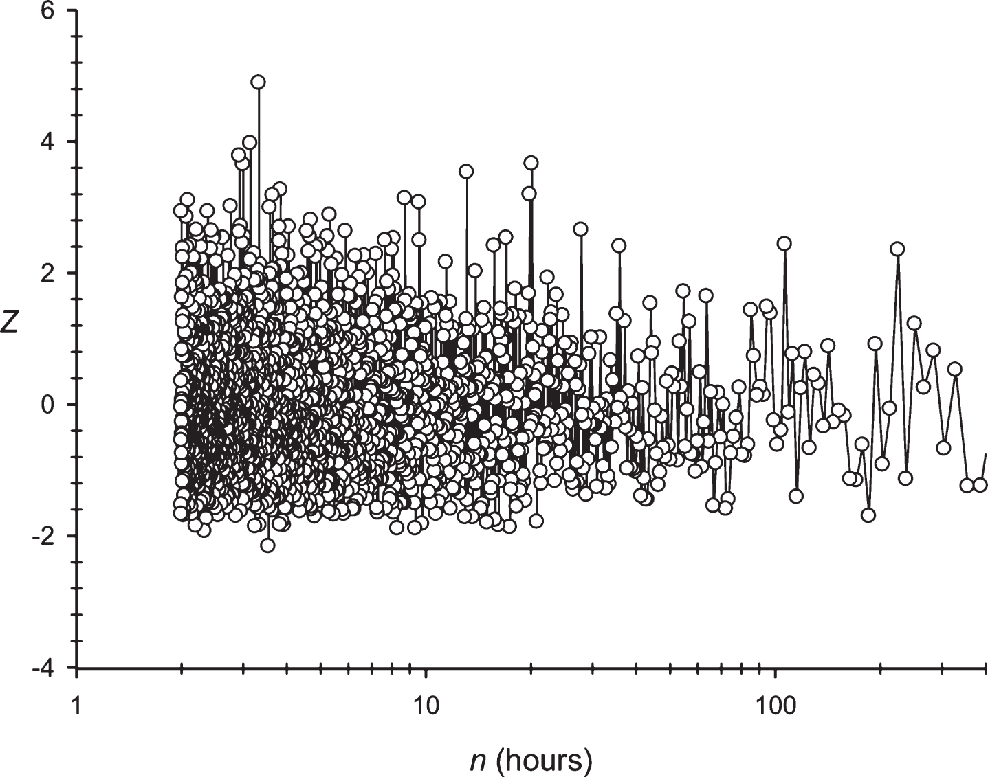
Figure 4 shows the results of the Fourier transform application to sequence A1, which created the sequence S1 basis. This figure demonstrates that the Z-values for various n-values do not exceed 5.0 and suggests that the Fourier transform is not capable of detecting the periodicity in sequence A1. This is due to the fact that the periodicity discovered using our method is characterized by insertions and deletions. Moreover, the insertions and deletions position was unknown before the sequence analysis.
Fig.4
The use of Fourier transform with the sequence A1 . The sequence S1 is a symbolical transformation of the sequence A1.
It is also interesting to consider the phase shifts of the discovered periodicity. The number of hours in a day (hours(i), i = 1,…,24) was numbered from 1 to 24, where the first hour of the day corresponds to one. Figures 5 and 6 show the difference between the column number k(1), which corresponds to the first hour of the day; and the number of first hour of the day hours(1) = 1. In the case of periodicity, the 24 and 25 h pattern of phase shifts is more complex. In the case of a periodicity equal to 24 h, Fig. 9 shows that the periodicity phase is relative to the number of hours of the day and remains the same for 4-5 days. After that, the 3 –6 h phase shifts occur. In the case of periodicity equal to 25 h each day, a stable phase shift occurs for some hours. This means that the periodicity phase was changing each day with the 25 h periodicity.
Fig.5
The phase shift for the periodicity with length equal to 24 h, in the sequence S2 is shown. The X-axis shows the number of the day in a region where there is a periodicity of 24 h. The Y-axis shows the difference between the hour of day at the time of opening of the candle and the column number.
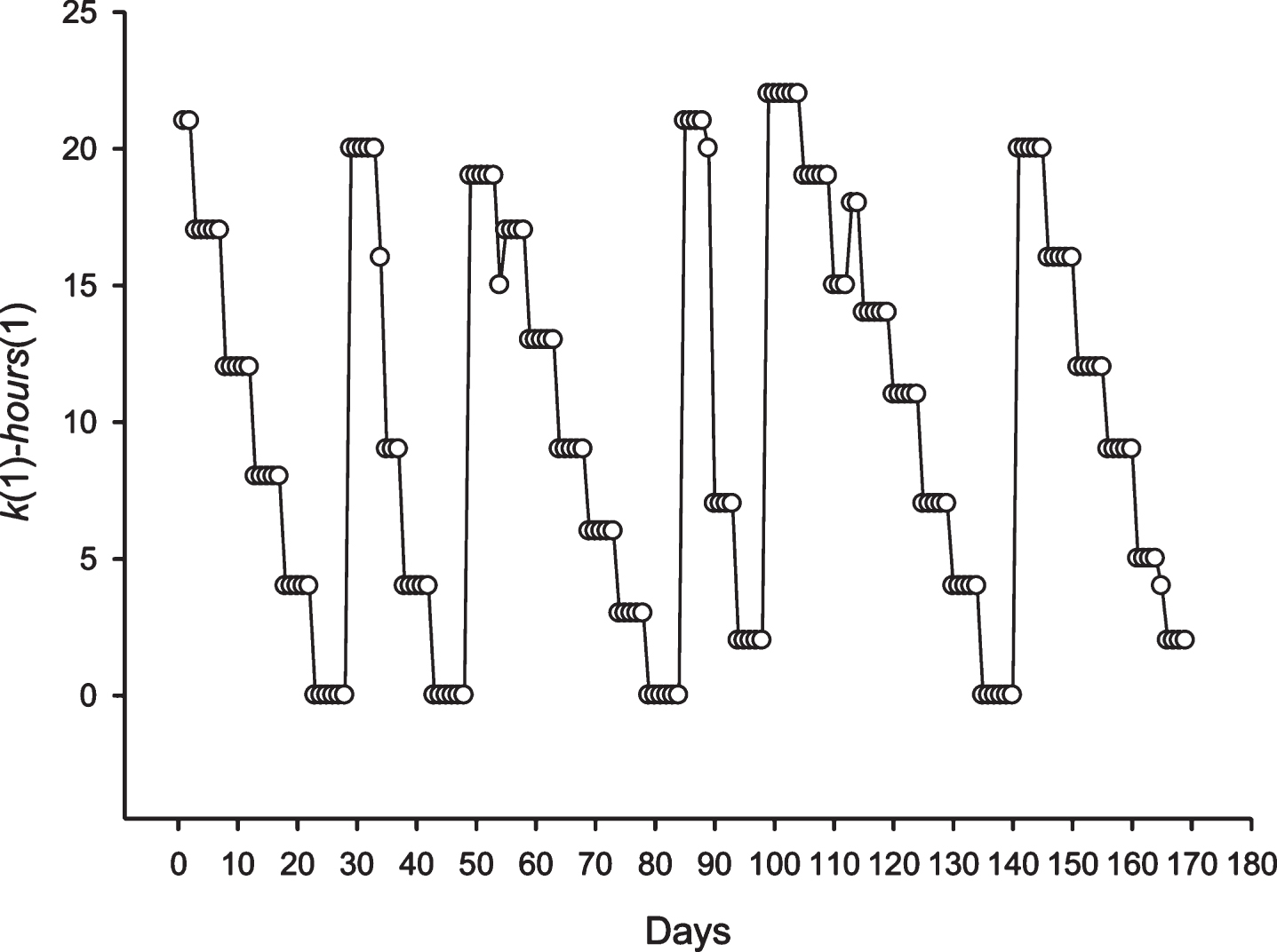
Fig.6
The phase shift for the periodicity with length equal to 25 h in the sequence S2 is shown. The X-axis shows the number of the day in an area where there is a periodicity of 25 h. The Y-axis shows the difference between the hour of day at the time of opening of the candle and the column number.
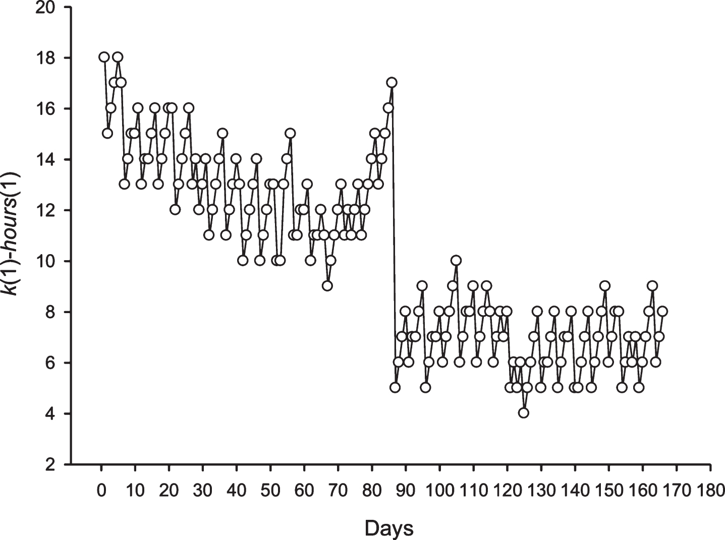
Fig.7
The spectrum of Z(n) obtained for the sequence S8 (candle is equal to 0.5 h)
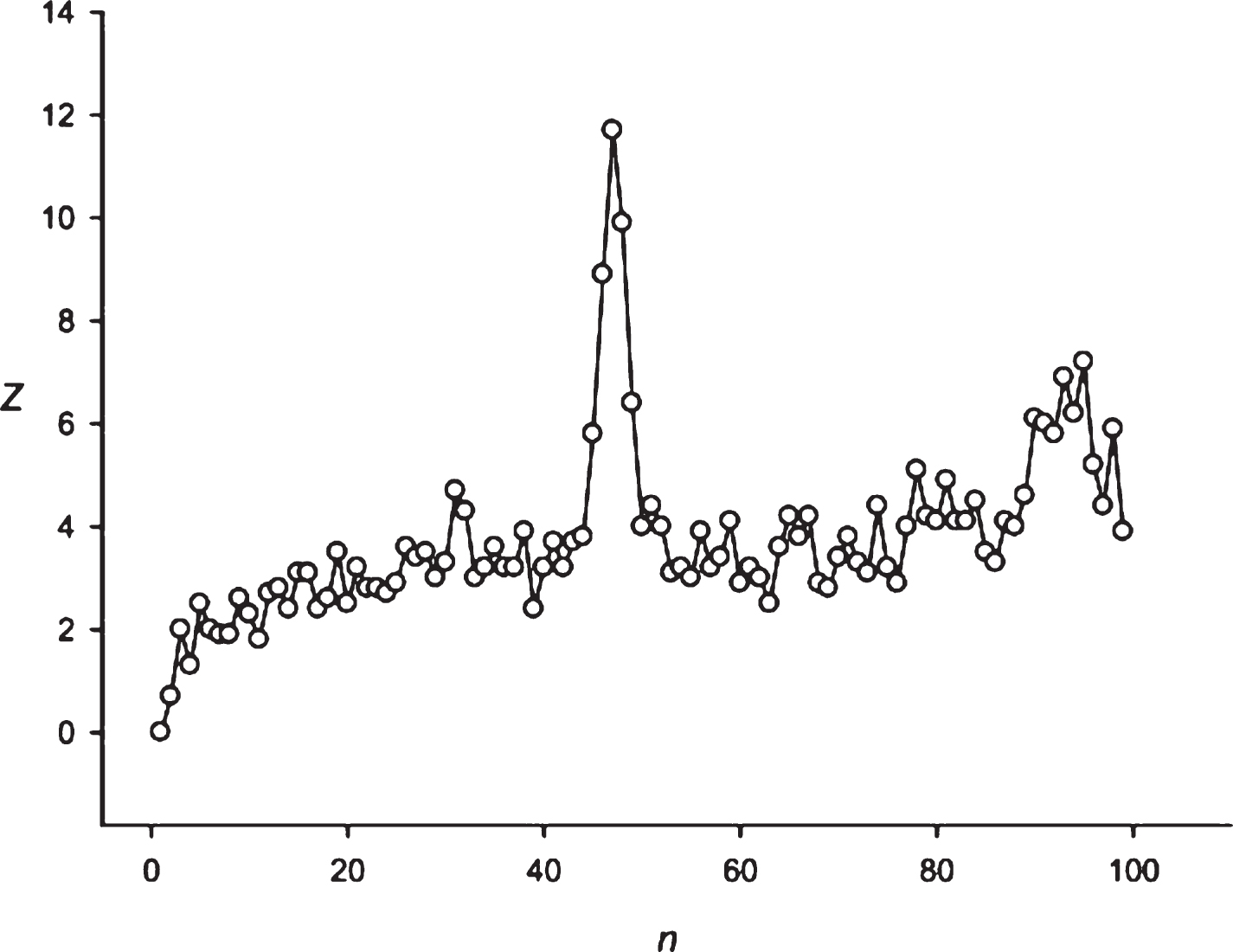
Fig.8
The spectrum of Z(n) obtained for the sequence S9 (candle is equal to 4 h).
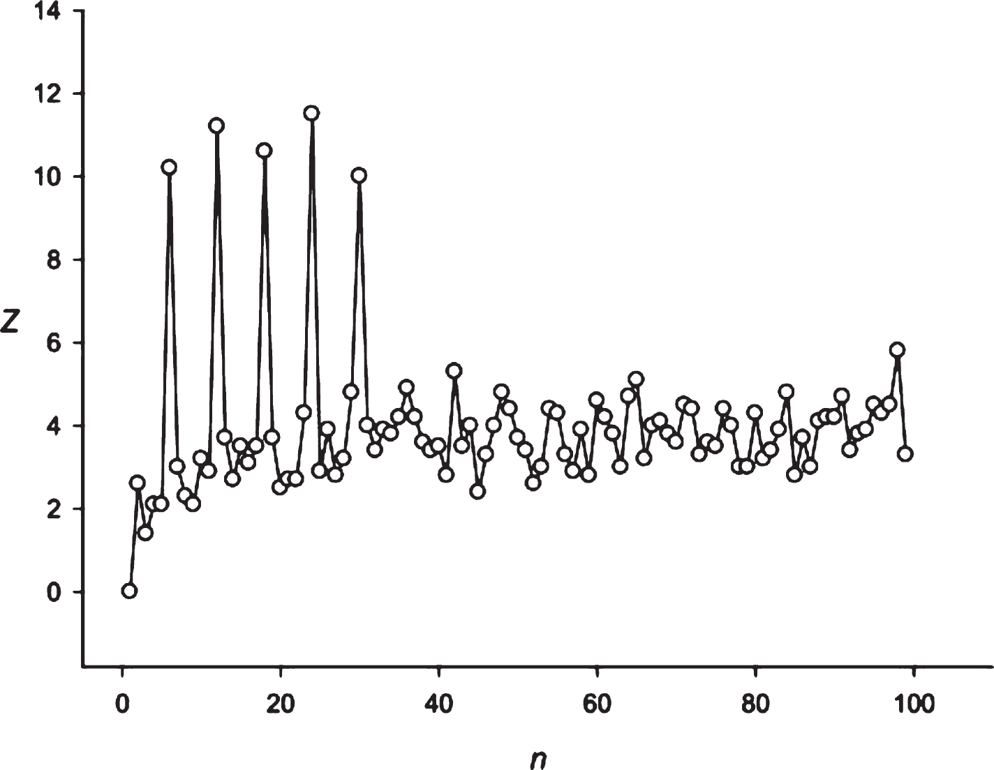
Fig.9
The spectrum of Z(n) obtained for the sequence S2 (stock of Bank of America).
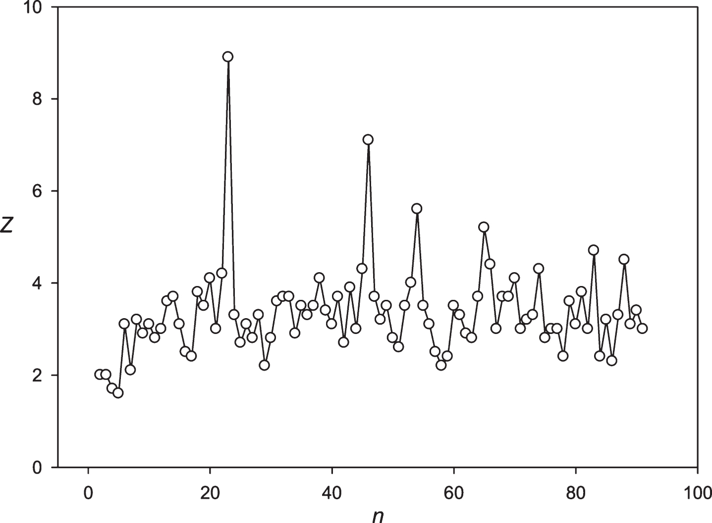
It is interesting to observe the presence of periodicity equal to 24 hours in different financial time series. To answer this question, we primarily employed the candles separated by the intervals of 0.5 h and 4 h for the Euro/Dollar (Eu/$) exchange rate. If the 24 hours periodicity is maintained, then it should be equal to 48 points (48×0.5 h = 24 h) and 6 points (6×4 h = 24 h). It is possible to see from Figs. 7 and 8 that the periodicity equal to 24 h is represented by these candles. Multiplicity periodicities of 24 hours could also be observed in Fig. 8 (48, 72, 96, 120 hours).
Then we decided to analyze the presence of periodicities equal to 24 hours in stocks randomly selected with several leading companies. The analysis was performed using the stocks of the Microsoft Corp. and the Bank of America. The results are presented in Figs. 9 and 10. These companies’ stocks are traded during the business day. So, in regard to these entities we registered about 7 candles for 1 hour each day. Data on trading these stocks within another time frame is missing. It means that the 24 hoursperiodicity could be observed as a periodicity equal to 7 points in regard to these corporations. It could be seen in Figs. 9 and 10. Then we examined the periodicities of S&P500 and NASDAG indices. These indices obtained about 8 candles for 1 hour each day. The 24 hours periodicity was transformed into the 8 points (one point is one candle) periodicity, which could be seen in Figs. 11 and 12. There is an extremely large value of Z(8); and also this periodicity induced overtones (4, 12, 16 points, etc.). Finally, we analyzed periodicities in the prices of gold and silver. Here we register 23 candles in average with the duration of 1 hour. This leads to the fact that the 24 hours periodicity becomes the periodicity equal to 23 points (Figs. 13 and 14).
Fig.10
The spectrum of Z(n) obtained for the sequence S3 (stock of Microsoft corp).
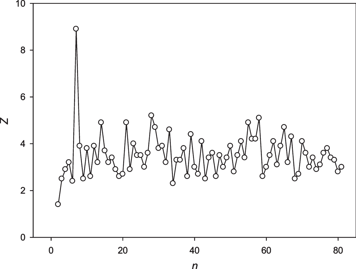
Fig.11
The spectrum of Z(n) obtained for the sequence S4 (S&P500).
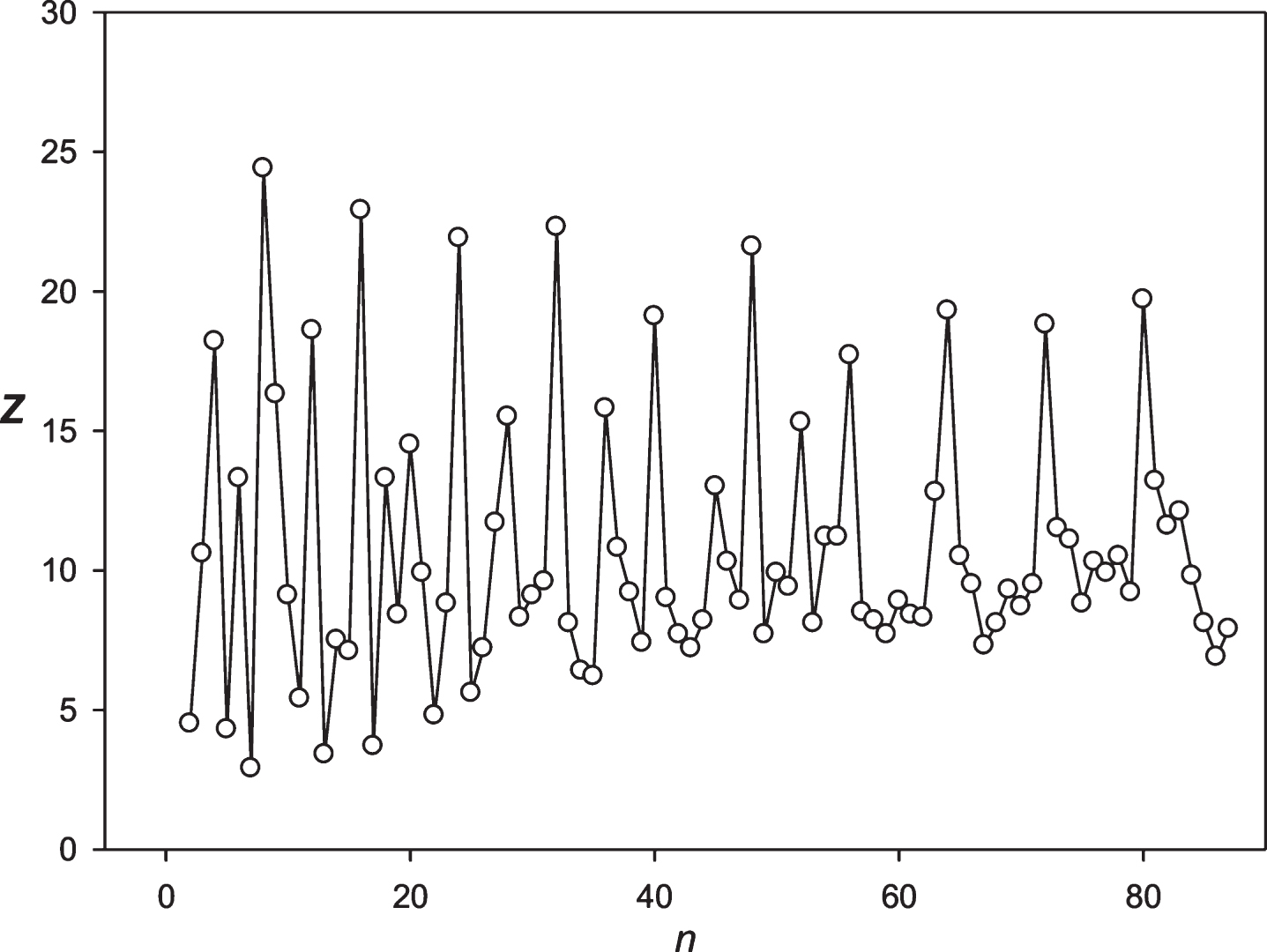
Fig.12
The spectrum of Z(n) obtained for the sequence S5 (NASDAG).
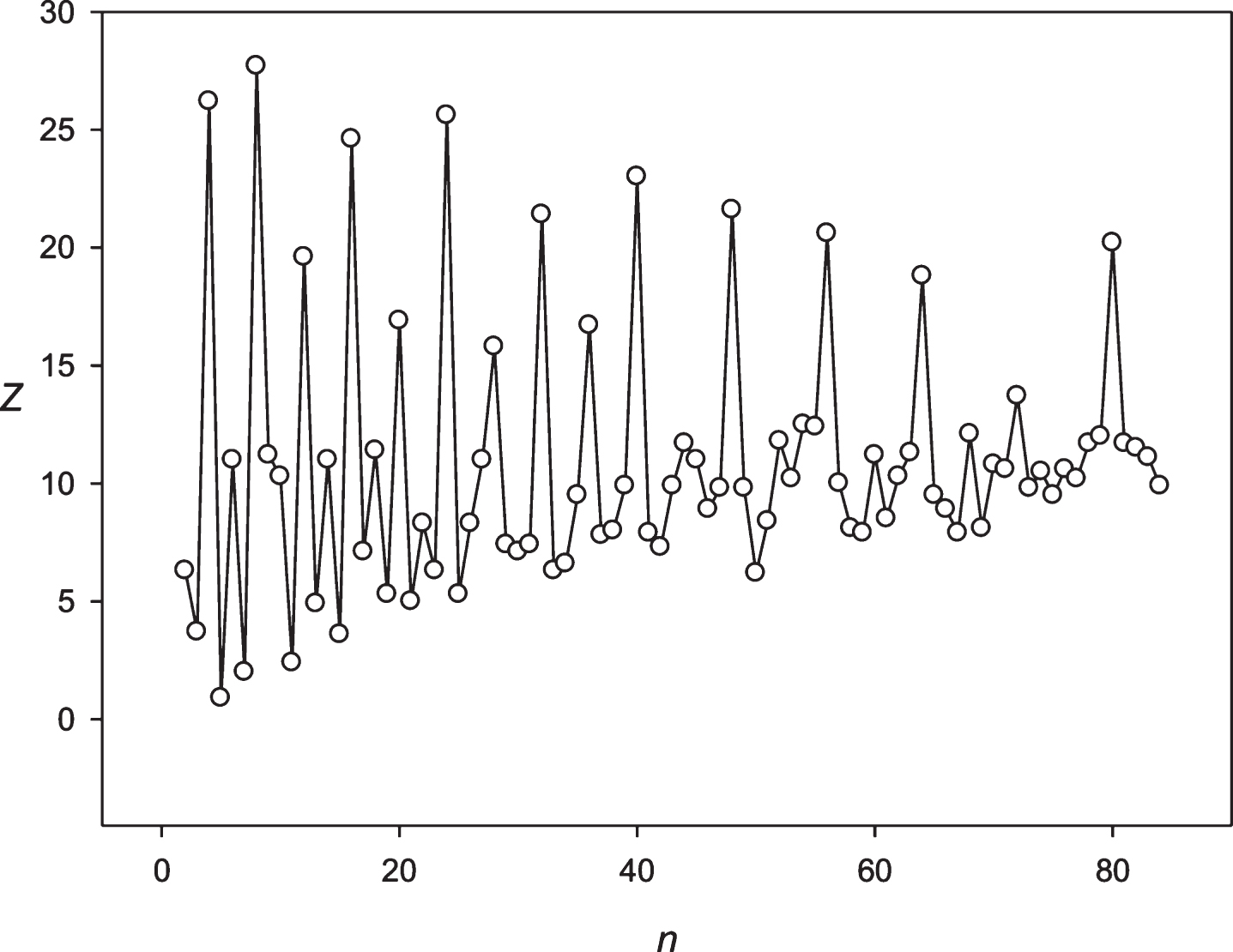
Fig.13
The spectrum of Z(n) obtained for the sequence S6 (Gold price).
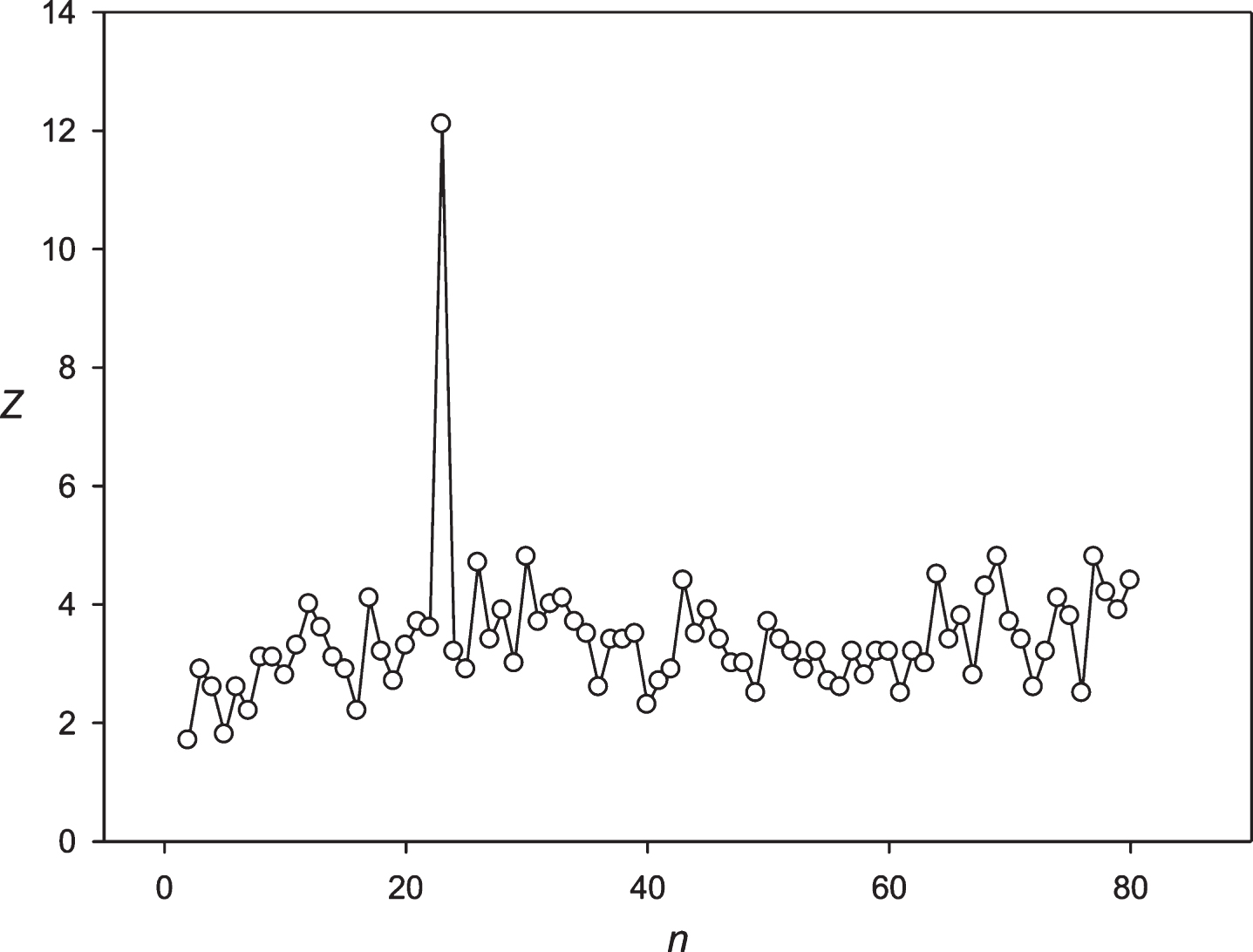
Fig.14
The spectrum of Z(n) obtained for the sequence S6 (Silver price).
All these periodicities could be found, if the symbols insertions or deletions are taken into account. The number of insertions or deletions for all alignments of the studied financial series ranged from 35 to 46. The size of a single insertion or deletion ranged from one symbol to 7 symbols. The question arises about the nature of the periodicity discovered in this work. The different periodicity processes is influencing the currency exchange rates. A person himself possesses the inherent rhythms of different frequencies; for example, Halberg (1969) classified the humans’ biological rhythms according to the periodicity length. He identified several groups of rhythms:
1. Low frequency group was characterized by periodicities ranging from 4 days to 12 months.
2. Mid-frequency group was characterized by periodicities ranging from 20 to 72 h.
3. High frequency group was characterized by periodicities less than 20 h.
Therefore, it could be assumed that the observed exchange rate periodicity at 24 and 25 h reflects the influence of the mid-frequency rhythms upon the exchange rate.
An attempt was made to find the periodicity for the sequence s(i) = x2(i)–x1(i),, where x1(i) and x2(i) are separated by minutes within the interval n from 2 to 70 min. No statistically significant periodicity was found within the given interval for a “minute” of the sequence.
It was also interesting to explain the presence of the symbols’ insertions or deletions (it was impossible to register frequencies without it) and the behavior of the phase shift for the periodicities of 24 and 25 h. Probably, there exists significant instability in the behavior of large human masses; and this instability could create phase shifts with insertions or deletions. Also, it could be assumed that certain events in public life might be the cause of phase shifts, insertions, or deletions. For a more accurate consideration of this issue, a separate study shall be required. The correlations between the phase shifts, insertions and deletions in the sequences S1 and S2 should be examined; as well as the events in public life and other factors of both social and physical nature.
This work was supported by the Russian National Foundation (http://www.rscf.ru/en). All calculations were performed at the supercomputer cluster of the Russian Academy of Sciences using 1000 processors (http://www.jscc.ru/eng/index.shtml). The web site (http://victoria.biengi.ac.ru/splinter/login.php) will be opened in 2017 and any user will be able to analyze any financial time series by the method developed in this paper.
References
1 | Benson G. , (1999) . Tandem repeats finder: A program to analyze DNA sequences, Nucleic Acids Res 27: , 573–580. |
2 | Chaley M.B. , Korotkov E.V. , Skryabin K.G. , (1999) . Method revealing latent periodicity of the nucleotide sequences modified for a case of small samples, DNA Res 6: , 153–163. |
3 | Chechetkin V.R. , Turygin A.Yu. , (1995) . Search of hidden periodicities in DNA sequences, J Theor Biol 175: , 477–494. |
4 | Chizhevsky A.L. , (1976) . The Terrestrial Echo of Solar Storms. Moscow. |
5 | Coward E. , Drabløs F. , (1998) . Detecting periodic patterns in biological sequences, Bioinformatics 14: , 498–507. |
6 | Dodin G. , Vandergheynst P. , Levoir P. , Cordier C. , Marcourt L. , (2000) . Fourier and wavelet transform analysis, a tool for visualizing regular patterns in DNA sequences, J Theor Biol 206: , 323–326. |
7 | Fadiel A. , Eichenbaum K.D. , Hamza A. , (2006) . “Genomemark”: Detecting word periodicity in biological sequences, J Biomol Struct Dyn 23: , 457–464. |
8 | Granger C. , Hatanaka M. , (1967) . Spectral analysis of economic time series, Ann Math Stat 38: , 288–293. |
9 | Halberg F. , (1969) . Chronobiology, Annu Rev Physiol 31: , 675–726. |
10 | Hamilton J.D. , (1994) . Time Series Analysis, Book, Springer Texts in Statistics. Princeton University Press. |
11 | Jackson J.H. , George R. , Herring P.A. , (2000) . Vectors of shannon information from fourier signals characterizing base periodicity in genes and genomes, Biochem Biophys Res Commun 268: , 289–292. |
12 | Korotkov, Korotkova, Kudryashov, (2003) . Information decomposition method to analyze symbolical sequences, Phys Lett Sect A GenAt Solid State Phys 312: , 198–210. |
13 | Korotkov E.V. , Korotkova M.A. , Tulko J.S. , (1997) . Latent sequence periodicity of some oncogenes and DNA-binding protein genes, Comput Appl Biosci 13: , 37–44. |
14 | Korotkov E.V. , Korotkova M.A. , Rudenko V.M. , (1999) . Latent periodicity of protein sequences, J Mol Model 5: , 103–115. |
15 | Kullback S. , (1997) . Information Theory and Statistics. Dover publications., New York. |
16 | Makeev V.J. , Tumanyan V.G. , (1996) . Search of periodicities in primary structure of biopolymers: A general Fourier approach, Comput Appl Biosci CABIOS 12: , 49–54. |
17 | Marple S.L. , (1987) . Digital Spectral Analysis: With Applications, Prentice-H. ed. |
18 | Miller W. , (2006) . An Introduction to Bioinformatics Algorithms, J Am Stat Assoc 101: , 855–855. |
19 | Mount D.W. , (2004) . Bioinformatics: Sequence and Genome Analysis. CSHL Press. |
20 | Oppenheim A.V. , Schafer R.W. , Buck J.R. , (1999) . Discrete Time Signal Processing Book, Pearson Education, Limited. |
21 | Polyanovsky V.O. , Roytberg M.A. , Tumanyan V.G. , (2011) . Comparative analysis of the quality of a global algorithm and a local algorithm for alignment of two sequences, Algorithms Mol Biol 6: , 25. |
22 | Pugacheva V.M. , Korotkov A.E. , Korotkov E.V. , (2016) . Search of latent periodicity in amino acid sequences by means of genetic algorithm and dynamic programming, Stat Appl Genet Mol Biol 15: (5), 381–400. |
23 | Rackovsky S. , (1998) . “Hidden” sequence periodicities and protein architecture, Proc Natl Acad Sci U S A 95: , 8580–8584. |
24 | Rastogi S.C. , Mendiratta N. , Rastogi P. , (2006) . Bioinformatics Methods and Applications: Genomics, Proteomics and Drug Discovery. PHI Learning Pvt. Ltd. |
25 | Stankovic R.S. , Moraga C. , Astola J. , (2005) . Fourier Analysis on Finite Groups with Applications in Signal Processing and System Design. John Wiley & Sons. |
26 | Stoica P. , Moses R. , (2005) . Spectral Analysis of Signals. Prentice Hall, New-York. |
27 | Struzik Z.R. , (2001) . Wavelet methods in (financial) time-series processing, Phys A Stat Mech its Appl 296: , 307–319. |
28 | Suvorova Y.M. , Korotkova M.A. , Korotkov E.V. , (2014) . Comparative analysis of periodicity search methods in DNA sequences, Comput Biol Chem 53: (Pt A), 43–48. |
29 | Turutina V.P. , Laskin A.A. , Kudryashov N.A. , Skryabin K.G. , Korotkov E.V. , (2006) . Identification of amino acid latent periodicity within protein families, J Comput Biol 13: , 946–964. |

