
The network of the Italian stock market during the 2008–2011 financial crises
Abstract
We build the network of the top 190 Italian quoted companies during the two financial crises of 2008-2009 (US credit crisis) and 2010-2011 (European sovereign debt crisis) and compare its structure to the pre-crises years, using both minimum spanning trees and the full network with thresholds. We also analyze the centrality and compactness of industry sectors. We find a general contraction of the network during the crises, both numerically due to stronger correlation as well as topologically, with the appearance of central dominant companies which attract the other ones into a very large cluster, dominated by financial institutions (commercial banks and insurance companies). In particular, we note the role of insurance behemoth Assicurazioni Generali, which rises from a pre-crises subordinate role to become the central company in the minimum spanning tree after the crises period. The few sectors which maintain compactness before and during the crises are utilities, publishing, and construction.
1Introduction
A long-standing empirical literature in finance has been challenging the validity of predictions of standard asset pricing theory and pointed to a long list of so-called market anomalies (see reviews in Fama (1991; 1998)). One interesting anomaly is related to institutional features that could have an important role in the stock price dynamics, causing stock price changes (returns) to comove much more than what is implied by economic fundamentals (Barberis and Shleifer, 2003; 2005). More recently, Anton and Polk 2014 have shown that stocks are connected through mutual fund owners and that the degree of shared ownership forecasts cross-sectional variation in return correlation, controlling for exposure to systematic return factors and other individual characteristics. The practical implication of this fresh evidence is to implement an active stock trading strategy that exploits the information contained in company ownership connections.
Motivated by these empirical findings, in this paper we study stock comovement, building a network based on the log difference of stock prices as in Mantegna 1999, who proposes building a correlation matrix of log-returns, an induced distance and consequently a network of companies. As the correlation matrix is dense and the resulting network would have an overwhelming amount of linkages, Mantegna suggests building a minimum spanning tree (Gower and Ross, 1969) which can give an overview of the structure without cycles, which is therefore very comprehensible for professionals. On the other hand, a minimum spanning tree’s (MST) displayed information is partial, as it sacrifices for readability purposes some potentially strong relations hiding them; therefore, it is usually coupled with a linkage’s reliability measure (Tumminello et al., 2007).
Network analysis has been used to study stock market dynamics in the last decade. The New York Stock Exchange, for its large size and importance among world capital markets, has attracted the attention of several researchers (Heimo et al., 2007; Onnela et al., 2003; Tumminello et al. 2005; Brida and Risso, 2010a; Gan and Djauhari, 2015). Further papers have applied network analysis to study different stock market economies (Huang et al., 2009; Tabak et al., 2010; Gałązka, 2011; Coronnello et al., 2005; Zhuang et al., 2008; Brida and Risso, 2010b; 2016). More recently, researchers have directed their attention to analyzing a stock market’s network at the time of financial market turbulence, such as that observed during the 2008-2009 US subprime financial crisis (Majapa and Gossel, 2016; Nobi et al., 2014; Khashanah and Miao, 2011; Wiliński et al., 2013). The Italian stock market is certainly under-researched, due to its small size and to the lack of reliable historical data (Coletti and Murgia, 2015). The few papers that focus attention on Italian stocks are by Brida and Risso (2007; 2009), who used a symbolization technique on Yahoo!’s data for a set of a few companies and for a relatively short time. Another stream of studies on the Italian market have built alternative networks based on boards of directors’ characteristics (Grassi, 2010), and company ownership structure (Piccardi et al., 2010).
Another group of studies focuses on methodological aspects and analyzes the different methods and techniques to build stock market networks. For example, Bonanno et al. (2004) compare different time frames, Coronnello et al. (2005) compare different clustering techniques, while Onnela et al. (2003a) propose the introduction of cliques in minimum spanning trees.
The literature on network analysis during financial crises includes studies on the South African and Korean markets (Majapa and Gossel, 2016; Nobi et al., 2014). Some papers also looked at the impact of the 1987 US stock market crash (Onnela et al., 2003b) showing a distinct pattern of increasing stock return correlations. This result is also known in the international finance literature, which shows that during crises and increased financial market volatility both individual stocks and market indexes’ correlations tend to increase significantly, thus reducing the benefits of cross-country diversification exactly when it is needed the most (Bekaert et al., 2009). This is instead not observed by Sandoval 2013 in his analysis of the network of stock markets’ indexes. Majapa and Gossel 2016 analyze 100 companies listed in the South African market and show a significant increase in MST clustering, in particular for banks, insurance, other financial firms and resource companies. Nobi et al. (2014) build the network of 185 Korean companies and find that the network has several clusters. During crises, stocks comove together into a single cluster, and this is specifically so for finance, heavy industry, construction and service sectors. Heiberger 2014 analyzes the network of S&P 500 companies in the US stock market. His findings show that before a crisis period many fragmented clusters are prevalent, whereas a centralized network emerges as a distinct result during the crisis, which is consistent with higher correlation and asset prices comovement during times of financial turmoil. The empirical studies that adopt network analysis all seem to reach conclusions that are consistent with stylized facts in the international empirical finance literature. Similar results on the MST are also presented by Wiliński et al. (2013) and Sienkiewicz et al. (2013), respectively on 562 listed companies of the Frankfurt Stock Exchange and 142 quoted companies of the Warsaw Stock Exchange. Both papers present the case of a company moving from a marginal role in a multi-cluster MST before the crisis to a pivotal role in a strongly centralized MST during the crisis. In the German stock market that was the case for a steel company, while it was a financial firm in the Polish stock exchange. These results share a common economic phenomenon. The shock that follows a financial crisis generates significant changes in the role that industry sectors and individual stocks play within the country’s stock market, and, as a consequence, we observe a reshaping of the asset market correlation structure.
In this paper, we study the Italian stock market during the two recent financial crises of 2008-2009 (US subprime credit crisis) and 2010-2011 (European sovereign debt crisis) and compare its structure to the pre-crises period of 2004–2007. Our methodological approach is largely the one proposed by Sandoval (2012a) that applies to a sample of the largestBrazilian listed companies. Sandoval builds a MST as well as the full network, using thresholds to filter out weak correlations. Moreover, in the case of MST and the full network, we study the consequences of financial crises on the centrality of economic sectors. Our study exploits a novel and higher quality dataset of the Italian stock market with respect to past studies that rely on small samples and a short time span. However, the database includes pre- and post-crises periods, that were not used in previous studies. The dataset we rely on is illustrated by Coletti and Murgia 2015. It has been carefully checked, specifically for aspects related to right issues, stock splits, dividend payments, and mergers and acquisitions, that very frequently are the sources of data errors in commercial databases.
We expect to find similar results to the extant literature, in particular the significantly higher correlations that are often presented in the international finance empirical literature. Moreover, as it seems that a stock market tends to reshape its topology during a crisis (Khashanah and Miao, 2011), we anticipate that this will be the case for the Italian stock market. Further, as observed in existing studies, we expect to find a switch from a clusters-dominated MST to a superstar-like MST. If this phenomenon is confirmed it can be exploited in portfolio management applications. Specifically, it could help to signal the evolution of stock market networks and to predict when the market is switching to a crisis period.
The paper proceeds as follows. Section one presents the Italian market database and illustrates the main techniques we use to obtain clean and error-free stock returns1. The second section constructs the correlation matrix using a metric distance, presents the building of the MST and its reliability measures and the definition of the measures which will be used to summarize and compare the networks. The third section shows the results for the MST and the fourth one for the full network. The concluding section sums up the paper’s main contributions and presents a few proposals for future research.
2Data
The data used in this paper are taken from Coletti and Murgia 2015, a comprehensive database of the Italian stock market. The data are thoroughly double-checked against available commercial databases and hand-filled with missed data from historical publications and Italian stock exchange data sources. We extract individual stock adjusted daily prices, dividend payments, and industry classification according to Fama and French 1997 for the 3-year period of June 2008 to May 2011. Differently from past studies (Sandoval, 2012a), we opt to analyze a longer time period in order to increase the sample size and minimize the impact of the short-term volatility that is observed during the financial crises periods.
The dataset has been filtered further by:
– excluding non-common stocks, such as preferred, savings (“risparmio”) and shares with special dividend rights, which typically represent a small percentage of company equity and are highly illiquid;
– excluding listed stocks of non-domestic companies, for which the Italian stock market is only a secondary exchange;
– excluding 137 stocks that have less than 630 observations, corresponding roughly to 30 months of data2 out of 36. Most of these companies are illiquid stocks. Many of these stocks have been suspended from listing for long periods and some of them started trading after June 2008 or were delisted before May 2011. We take a less strict approach than Sandoval (2012a) when excluding stocks that have a single missing day. This would avoid removing companies that faced a few trading halts for technical reasons.
From the remaining 249 stocks sample, we sort them according to the period’s average market capitalization and select the 190 with the largest market value. Thus, we construct the sample as in Sandoval (2012a) and are able to make meaningful comparisons with his results. The final sample of Italian companies is presented in the Appendix.
We use the industry sectors taken from the macro-classification of Fama and French 1997. No company changes sector in the sample period. If a company is a holding, it is classified according to its prevalent underlying economic activity, setting it to “Trading” when no prevalent activity is evident. In the same way, several banks are classified as “Trading” when their market-based financing is largely prevalent over the deposit-taking activity.
As is common in finance empirical analysis we use adjusted daily stock returns. We correct prices for dividends using the formula
Then, prices are also adjusted for capital changes, such as a cash equity issue, pure right or mixed issues and stock splits. Adjustment factors are taken from AIAF 2014 and their function is to ensure that the stock theoretical market capitalization betweencum-day and ex-day that overlaps with the capital change transaction remains constant.3 For each factor k with ex-day T we apply the formula
Finally, we compute daily log returns as follows:
For each stock in the sample we have available a time series of 762 daily returns. Missing returns are on average 0.73% with a maximum of 15.5% for company SAT –Aeroporto Toscano Galileo Galilei (TSA). We follow the idea originally proposed by Mantegna 1999 and calculate pair correlations ρij between each couple of stocks i and j. As in most studies, we opt to compute Pearson’s correlations instead of Spearman’s correlations used by Sandoval (2012a). According to experiments by Sandoval 2013, the induced network does not differ from the one produced using Pearson’s correlation. To double check it in our case, we rebuilt the crises’ MST using Spearman’s correlation and obtained the same tree for what concerning the reliable linkages.
As correlation takes values between -1 and +1, we can define a metric distance4
The same procedure is applied to 190 stocks listed in the pre-crises period of June 2004 to May 2007, in order to make a meaningful comparison between pre- and post-crises times. We attempt to keep the same companies in the pre- and post-crises sample; however for 47 stocks we had to replace them as they were not listed in 2004 or they did not match our selection criteria. Table 3 in the Appendix presents the complete list of analyzed stocks.
3Network construction
The distances matrix introduced in the previous section allows us to build a minimum spanning tree. We build it using Kruskal’s algorithm (Kruskal, 1956): starting from 190 isolated nodes, we select 189 edges in increasing distance order, skipping the ones that lead to a cycle. This is an easy algorithm with complexity o (n2 log n), where n is the number of nodes, which guarantees a connected tree without cycles and planar. The tree can be represented using a traditional graph picture, in which each node can also be colored according to its industry sector.5 The MST permits to define a subdominant ultrametric distance (Mantegna, 1999; Mantegna and Stanley, 2007; Rammal et al., 1986) as
We then check link reliability using two bootstrapping strategies. The first is a simple procedure: we build 100 completely random time series, using the same frequencies of correlations as the original ones, and build their distances’ matrixes. We calculate the minimum distances in these matrixes and subsequently their average which is 1.3523, which corresponds to a correlation coefficient of 0.0856. This is the average of the best distances obtained randomly and thus we claim that everything above this distance could have been randomly generated. In our MST no linkage has a distance above this level, thus no linkage can be considered to be purely random. On the other hand, the full network has 8.4% linkages whose distance is above 1.3523, that are thus eliminated.
The second bootstrap method deals with the problem that MST edges can be plagued by random noise, since the Kruskal algorithm does not choose all the best edges, but potentially good linkages must be discarded if they lead to cycles. In order to distinguish between those chosen linkages which are undoubtedly the best ones from those which are chosen because they are slightly better than the other linkages connecting that node, we use the technique proposed by Efron 1979 and applied by Tumminello et al. (2007) and Kantar et al. (2011) to spot unreliable linkages. We create 1,000 random datasets picking, allowing repetitions, 762 days. In this way, in each dataset the same day’s return can appear several times or none. For each dataset, we then compute its correlation and distances matrixes and build its corresponding MST. Thus, we have 1,000 MSTs and a probability distribution of the edges in our MST, without having to infer the joint distribution from the theoretical distribution of r. Each edge appearing in our final MST will have a reliability score equal to the percentage frequency that this edge appears in the 1,000 MSTs. In our trees’ picture we use the edge’s thickness to represent it.
For the MST and the full network we calculate some standard graph measures. Our topological measures, which do not involve distances, are:
– node’s degree: the number of edges incident upon the node in the graph. The larger the degree, the more central and more connected the node is. The theoretical minimum value is obviously 1, while the maximum value for a MST is n - 1 (in the case of a star MST) and for a full network it is n. It is important to note that in a tree the average degree is always 2 - 2/n as the number of edges is fixed n - 1;
– node’s eigenvector centrality (Newmann, 2007) (Sandoval, 2013): this measure is determined considering the graph’s adjacency matrix and calculating the eigenvector corresponding to its largest eigenvalue. That eigenvector’s elements are the nodes’ eigenvector centralities. This is a measure which considers how central the node and its neighboring nodes are, thus expanding the degree concept;
– node’s centrality betweenness (Freeman, 1977) (Sandoval, 2012b): how many times the node is in the shortest path between the other two nodes divided by all the possible nodes’ couples. This is a centrality measure which focuses on spotting those nodes which act as bridges among several loosely connected parts of the graph.
Measures which involve the distance d or the correlationρ are:
– the node’s average distance from other nodes: the sum of distances in the shortest path from this node to each other node of the graph. This measure is used to spot nodes which are far away from the rest of the graph;
– the node’s strength: the sum of the correlations of a node, i.e. for node j it is ∑i≠jρij;
– the node’s closeness centrality (Sabidussi, 1966): the inverse of the sum of all distances to other nodes.6 It can be calculated for node j as 1/∑i≠jdij;
– the node’s k-shell weighted decomposition (Garas et al., 2012): this is a measure which makes sense only for the full network. Instead of following the standard k-core decomposition (Alvarez-Hamelin et al., 2005; Sandoval, 2012a) we prefer to use a decomposition which also takes into consideration the correlations as weights, in order to improve our results when we analyze strongly interconnected networks. We define the weighted degree for node j as
4MST results
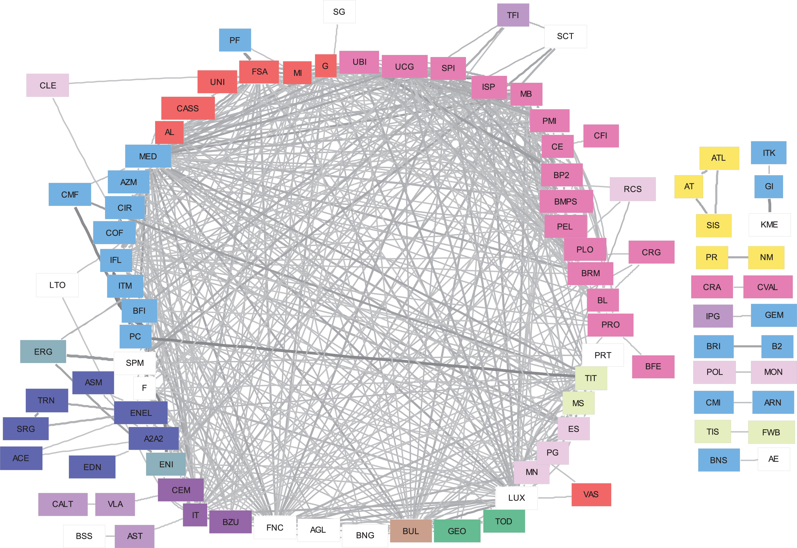
MSTs for the 2008–2011 and the reference 2004–2007 periods are presented in Fig. 1 and 2. In order to comment on them, we concentrate on the thickest linkages which are the most reliable. The most striking difference between the two figures is that during the crises period listed stocks tend to cluster around some dominant nodes as hubs, and these dominant nodes are often linked in a very reliable way among themselves. It is interesting to note that Assicurazioni Generali (G) stock plays a pivotal role. On the other hand, in Fig. 2 clusters appear larger and more scattered, with companies connected in rows and with interconnecting companies among hubs. In particular, the crises MST presents a central insurance companies hub with stocks of Assicurazioni Generali, Unipol (UNI), Fondiaria Sai (FSA), Milano Assicurazioni (MI) and Cattolica Assicurazioni’s (CASS). This is strongly connected with two large bank hubs through Intesa San Paolo (ISP) and Unicredit Group (UCG) stocks. Mediobanca (MB) has its own loosely connected non-bank hub. On the left, loosely connected with the rest, there is the Fiat (F) Pirelli (PC) hub with some companies related to the car and transportation manufacturing business, such as Piaggio (PIAG), Pininfarina (PINF) and Exor (EXOR). Also loosely connected with the rest there is the dipole ENEL and ENI, the two privatized, but still government controlled ex-monopolists of electrical power and gas, around which several utilities companies (blue) are strongly connected. The construction in dark purple and construction materials (light purple) cluster is built around Italcementi (IT) and Buzzi Unicem (BZU) which is weakly connected to a hub built on the axis SIAS (SIS), Autostrade (AT), CIR and Cofide (COF). The last cluster, linear instead of star-like, is the publishing sector with Mondadori (MN), Espresso (ES), RCS and Poligrafici Editoriale (POL) companies. On the other hand, the trading sector, in light blue color, being a catch-all sector with companies involved in several different sectors, is scattered across the entire tree. Quite unexpectedly, telecommunication companies are not grouped together.
Fig.1
Minimum spanning tree for June 2008 – May 2011. Colors represent sectors and edge’s thickness represents reliability.
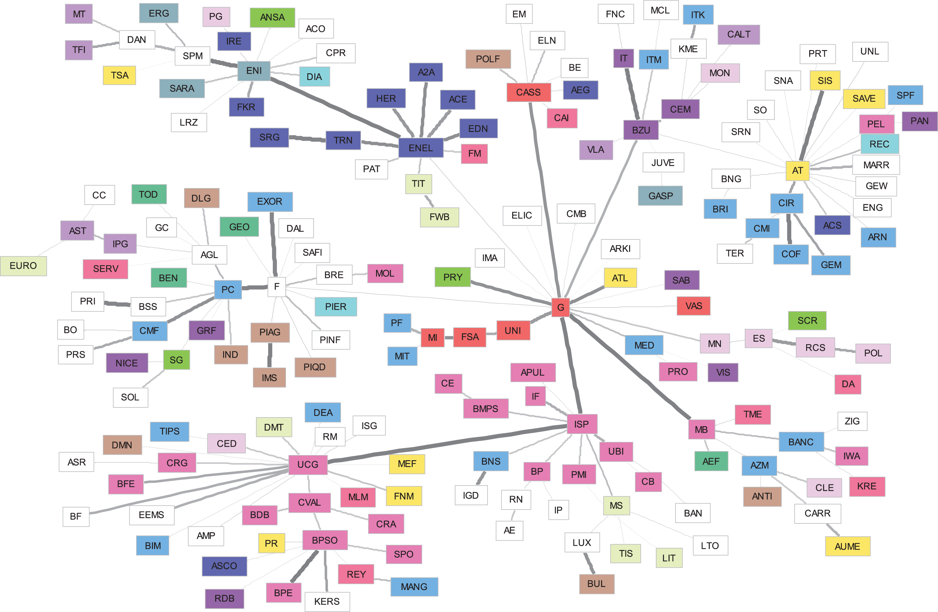
Fig.2
Minimum spanning tree for June 2004 – May 2007. Colors represent sectors and edge’s thickness represents reliability.
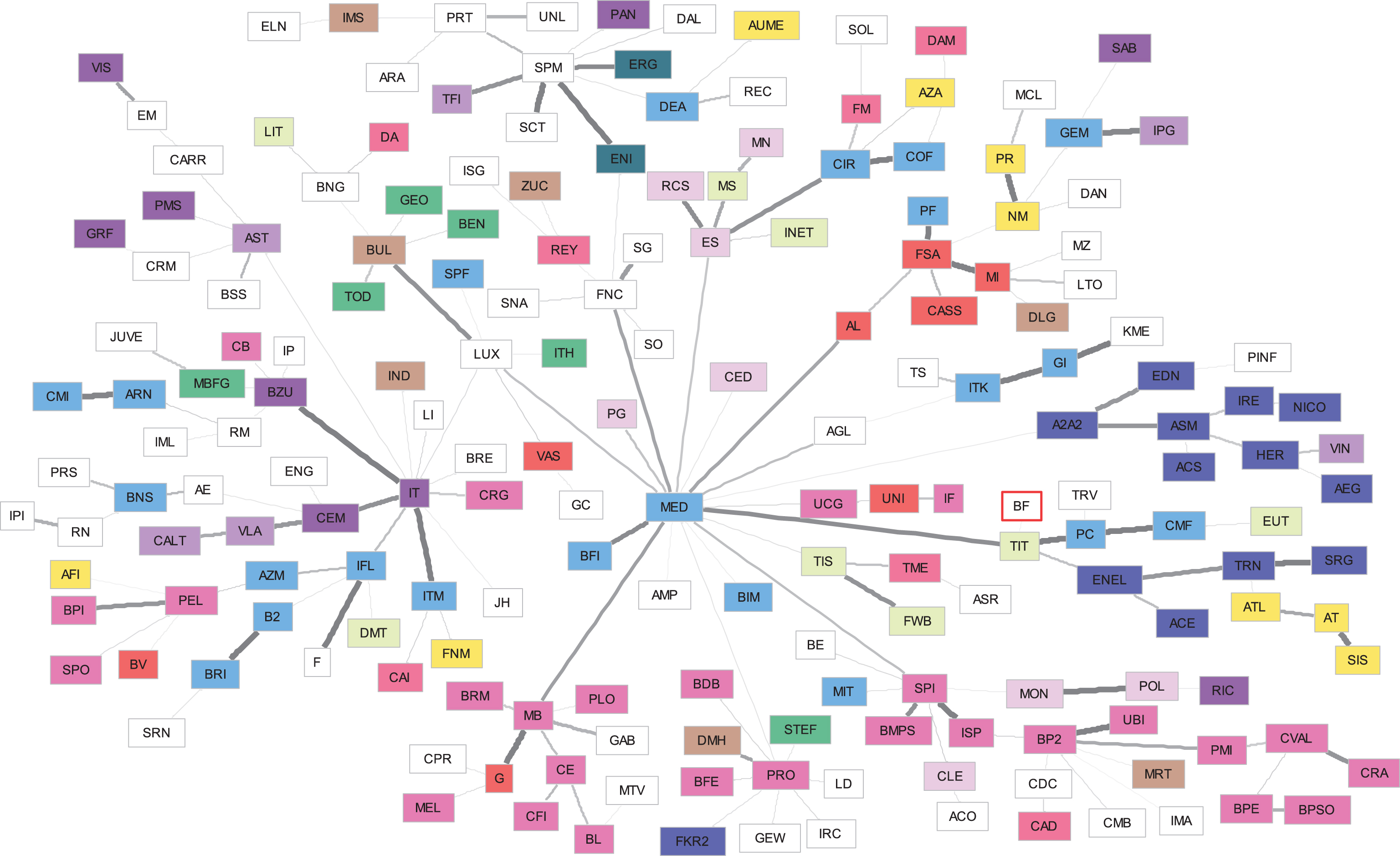
Comparing trees between pre- and post-crises, it is interesting to note that the utilities cluster still existed before, but without ENEL and without the connection with the petroleum and natural gas sector. The only other clusters which somehow existed before were the publishing sector (very light purple) and the strong construction sector (dark purple). Assicurazioni Generali (G) was not in a central position and was also in Mediobanca’s (MB) area of influence, disconnected from the insurance hub Alleanza (AL), Fondiaria Sai (FSA) and Cattolica Assicurazioni (CASS). Mediolanum (MED), a holding with significant participation in the banking and insurance sectors, seems to be the tree center.
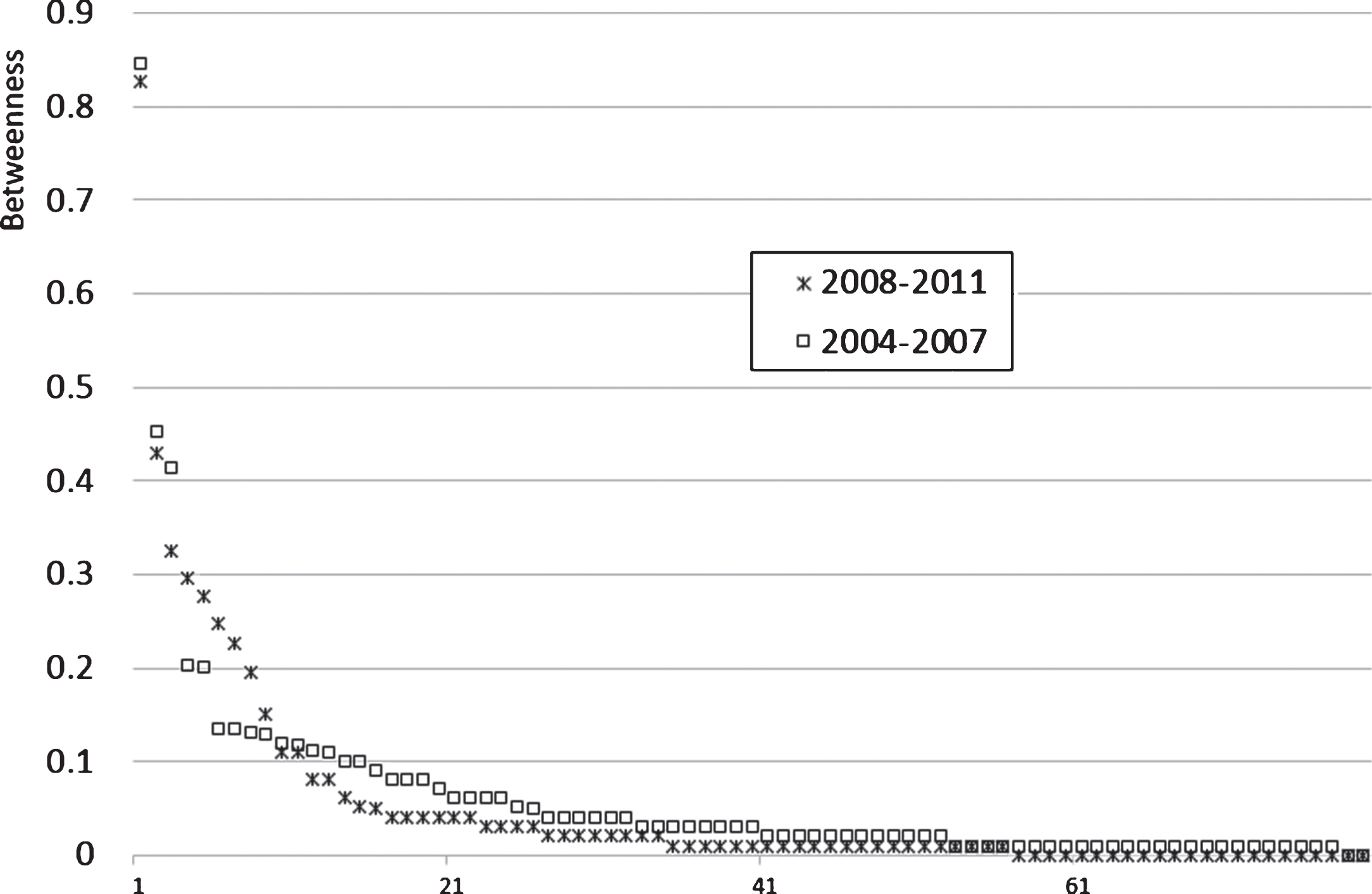
Visual inspection of a MST can hide some general characteristics, which appear clearer when using the graph measures illustrated above, whose distributions are shown in Figs. 3 - 10. From the degrees’ distribution, we immediately observe that during the crises the number of degree 1 nodes increases from 113 to 134, consequently reducing the amount of 2, 3, 4 and 5-degree nodes, as the total number of edges in a MST is constant. This is due to the presence of star-like hubs in the crises MST. Comparing our result with Sandoval’s evidence for Brazil in 2011 (Sandoval, 2012a), we observe that the Brazilian structure is much more similar to the Italian structure before the crises, with the presence of only 105 nodes with degree 1. On the other hand in Fig. 4, eigenvector centralities seem to be approximately the same ones pre- and during crises and very similar to Sandoval’s ones. Betweenness centrality in Fig. 5 shows the same situation as degree, but it is clearly amplified: during the crises we see a sequence of companies with large betweenness centrality, the ones which are at the center of the nodes, and then the rest of the nodes with slightly smaller betweenness centrality with respect to the pre-crises situation, as there are fewer nodes which act as bridges towards a single other node. In order to compare Sandoval’s results we need tomultiply our betweenness centrality by the number of possible node combinations, 190·189/2 and we see that the Brazilian distribution looks like the Italian pre-crises distribution.
Fig.3
Distribution of nodes’ degrees for the MSTs during crises and pre-crises.
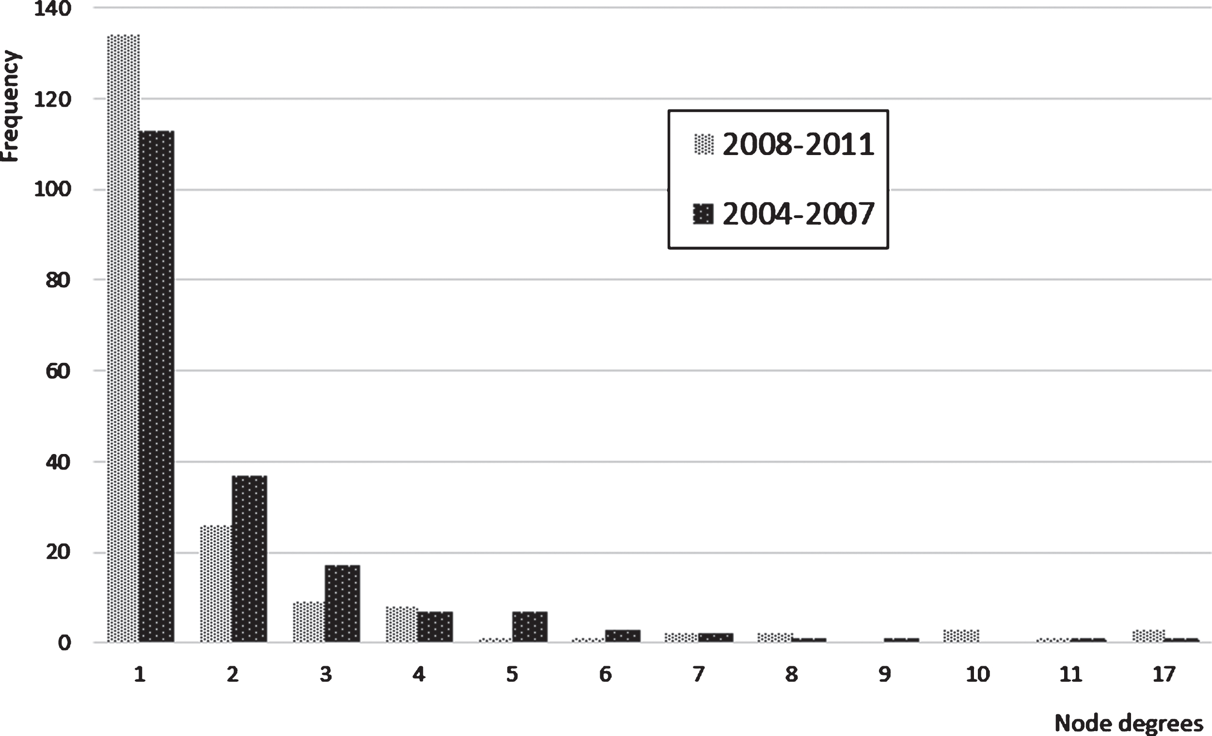
Fig.4
Distribution of nodes’ eigenvector centrality for the MSTs during crises and pre-crises.
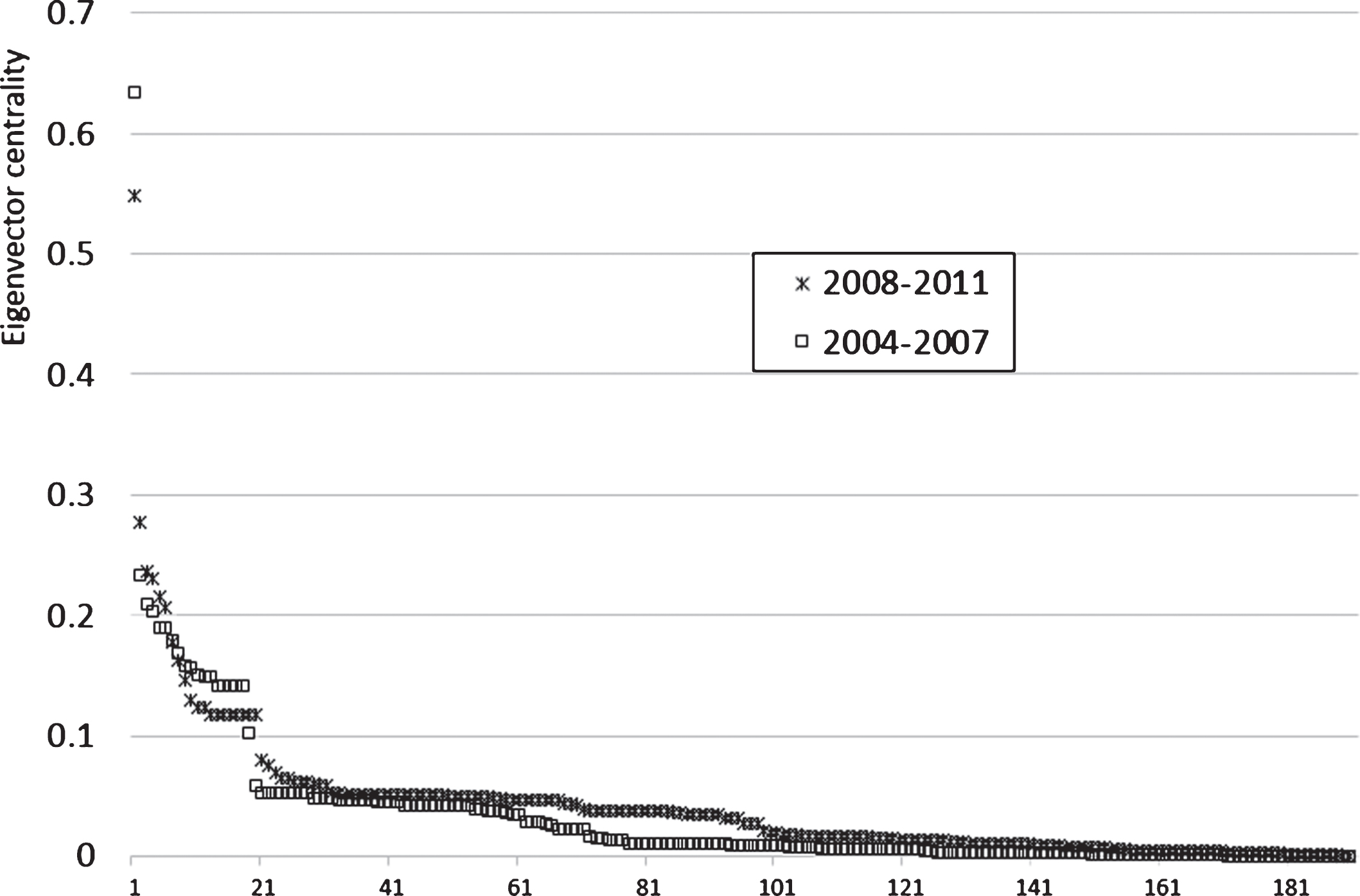
Fig.5
Distribution of nodes’ betweenness centrality for the MSTs during crises and pre-crises. Nodes after the 78th always have a betweenness of 0.
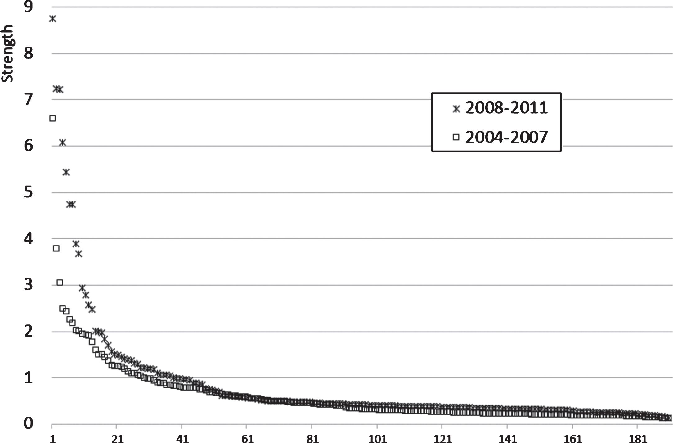
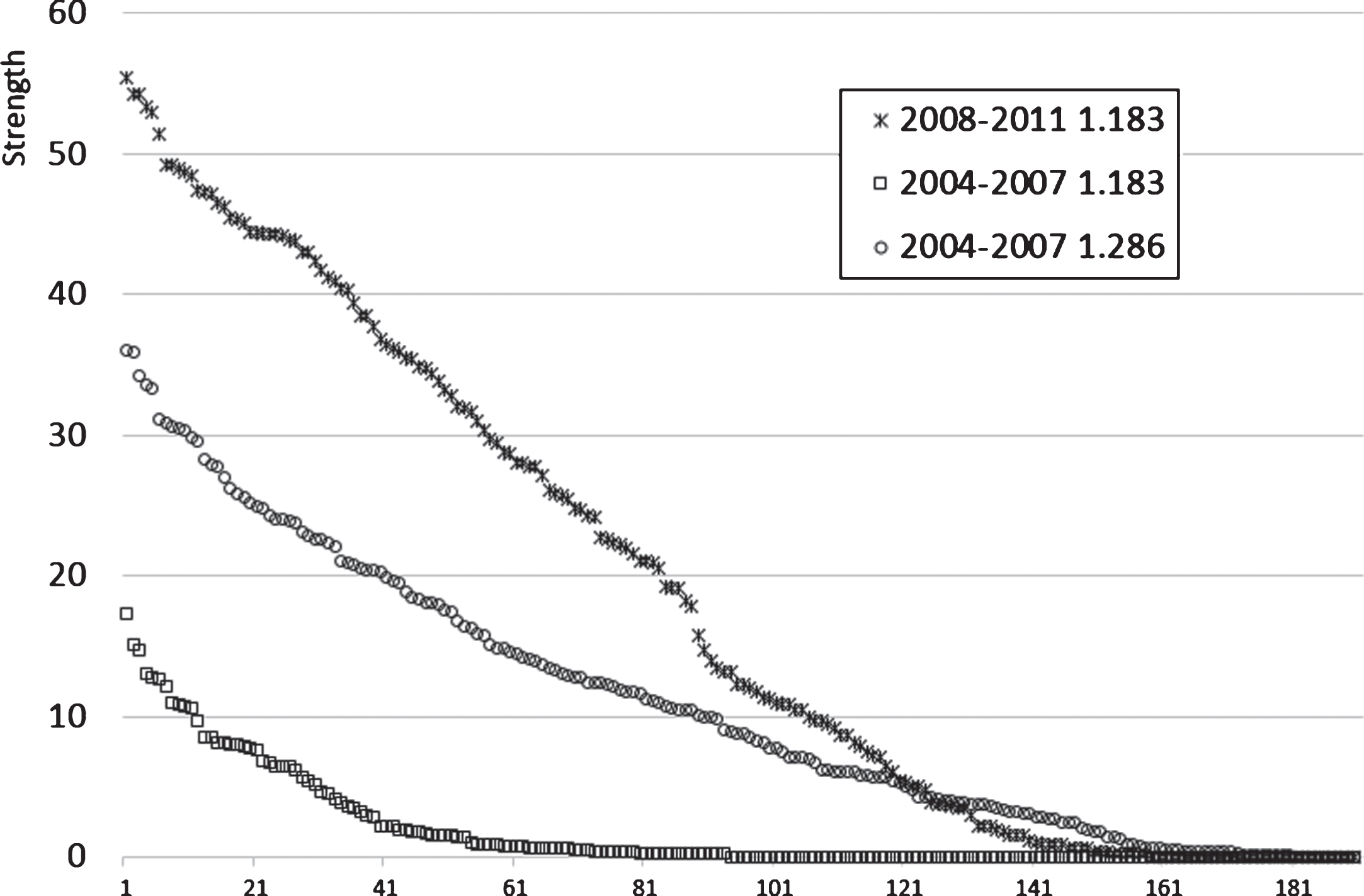
Switching to metric distances, the total distance of the MST drops by 9%, from 221 before the crises to 201 during the crises. Therefore, if the topological structures of the two MSTs were similar, we would expect a similar drop in the average distance of each node from the other ones. Looking at Fig. 6 we observe a general drop of 20% for the most far away nodes and even more for the other ones, meaning that the tree does not only have shorter distances but also shorter paths and is thus more compact. In Fig. 7 we depict the nodes’ strength which is, as expected, greater during the crises as correlations are larger. Our pre-crises situation is similar to the Brazilian market, in particular for large strength nodes. The same conclusions may be drawn for closeness centrality in Fig. 6.
Fig.6
Distribution of nodes’ average distance and closeness centrality for the MSTs during crises and pre-crises.
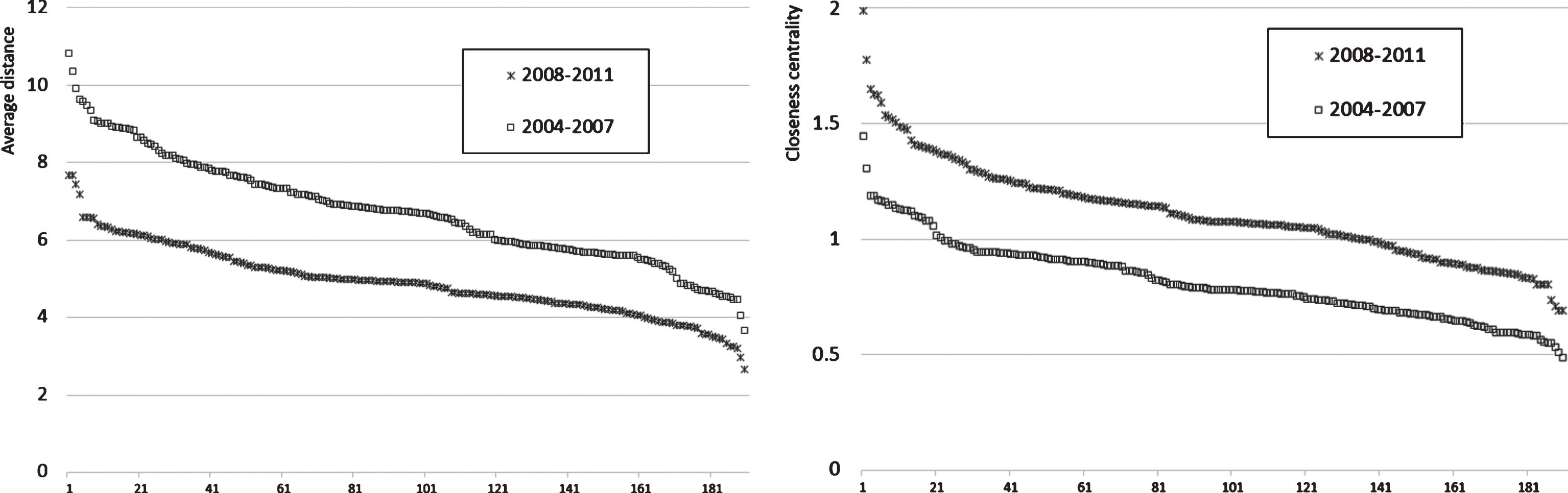
Fig.7
Distribution of nodes’ strength for the MSTs during crises and pre-crises.
In order to perform a deeper analysis of the trees’ structures, we analyze some measures by industry sector. In Table 1 we illustrate the average distance intra-sector for some sectors, i.e. calculated only among the sector’s companies. It is worth pointing out that for large sectors it is very difficult that this measure may be small, as it is easier to find one of the sector’s companies far away in the tree. We observe a general decrease in the average distance during the crises, with some sectors strongly reducing it, such as construction materials and transportation. The most striking sectors are, however, real estate, banking and in particular the insurance sector which drops from 12.21 to 5.23. This is also evident from the qualitative analysis of the MSTs, where Assicurazioni Generali (G) plays a key central role in the financial crises tree. We also checked the average distance intra-sector for the insurance sector without Assicurazioni Generali and it resulted in 5.46, meaning that it is the entire sector which is now more connected. A counter trend sector is the trading one, which is a catch-all sector for holdings and investment institutions.
Table 1
Average distance intra-sector, average degree by sector and average betweenness by sector, for sectors with at least 5 companiesfor the MSTs during crises and pre-crises
| June 2008 – May 2011 | June 2004 – May 2007 | |||||||
| Sector | Count | Average distance intra-sector | Average degree | Average betweenness | Count | Average distance intra-sector | Average degree | Average betweenness |
| Printing and Publishing | 8 | 10.34 | 1.75 | 1.4 | 8 | 8.09 | 1.88 | 1.8 |
| Consumer goods | 9 | 11.12 | 1.11 | 0.1 | 7 | 13.85 | 1.71 | 1.0 |
| Apparel | 4 | 8.35 | 1.00 | 0.0 | 6 | 8.35 | 1.17 | 0.2 |
| Construction materials | 9 | 11.83 | 2.11 | 4.2 | 9 | 16.43 | 2.89 | 6.4 |
| Construction | 6 | 13.72 | 1.50 | 0.9 | 6 | 14.56 | 1.83 | 1.4 |
| Machinery | 8 | 11.87 | 1.75 | 1.0 | 7 | 14.91 | 2.14 | 2.0 |
| Electrical equipment | 6 | 12.13 | 1.00 | 0.0 | 4 | 11.20 | 1.00 | 0.0 |
| Automobiles and Trucks | 6 | 9.42 | 3.00 | 5.3 | 5 | 11.49 | 1.20 | 0.4 |
| Utilities | 12 | 9.84 | 1.92 | 2.2 | 13 | 11.52 | 2.00 | 2.3 |
| Communication | 7 | 12.25 | 1.57 | 0.7 | 8 | 9.77 | 1.75 | 2.0 |
| Business Services | 8 | 11.78 | 1.13 | 0.1 | 7 | 13.82 | 1.57 | 0.6 |
| Transportation | 9 | 13.42 | 2.78 | 2.5 | 9 | 18.27 | 1.67 | 1.2 |
| Banking | 23 | 8.28 | 3.09 | 4.8 | 27 | 14.36 | 2.41 | 3.0 |
| Insurance | 6 | 5.23 | 5.33 | 16.4 | 8 | 12.21 | 2.50 | 4.2 |
| Real Estate | 5 | 12.31 | 1.20 | 0.2 | 7 | 20.05 | 1.29 | 0.7 |
| Trading | 22 | 14.62 | 2.05 | 1.7 | 22 | 12.89 | 2.91 | 5.9 |
The sum of degrees for a MST is fixed as the number of edges is 189: thus we observe in Table 1 a general decrease of the average degree for manysectors with a sharp increase for banking, construction materials, and especially insurance which doubles from 2.50 to 5.33. This effect is even more evident in betweenness centrality by sector, as in a tree the path between two nodes, without traversing the same edge twice, is unique, and therefore in a tree betweenness reflects degree distribution. Instead this is due to Assicurazioni Generali being at the tree’s center, as removing it from the sector’s average led to an average degree of 3.0 and a betweenness of 3.1, still large but smaller than banks.
4.1Ownership effect
When a strong relation exists between two listed companies, we observe a strong comovement between their shares’ prices. There may be, however, several explanations for the observed comovement. One of them is related to cross-ownership: a company owns an equity stake in the other or they share the same ultimate controlling shareholder. When news to one company reaches the market, both stocks will be affected. In order to identify such cases, we use ownership data that we retrieve from the CONSOB website (2016), the Italian Stock Market Authority, which lists all ownerships with at least 2% of voting rights7. Initially, we calculate the correlation between the direct ownership among companies and our prices’ correlation matrixes, obtaining 5.44% before and 2.73% during the crises. In order to consider also the frequent indirect ownerships by a non-listed company or person, for each couple of companies A and B owned by a third subject C, we add to our two ownership matrices the minimum between the ownership of C on A and of C on B. Recalculating the correlation of these new ownership matrices with our prices’ correlation matrixes, we get 6.98% before and 4.80% during the crises. All these correlations are significantly different from 0 at 1/1000 level. This means that there is in general a significant effect of ownership on correlations, even though the effect is responsible, on average for less than 7% of the correlation’s value. Very interestingly the effect almost halves during the crises, probably because the general market effect overwhelms the ownership’s effect.
In order to analyze the effect of ownership on the MSTs and networks, we take into account all the ownerships with at least 10% of voting rights. We built the ownerships’ networks for the 2004–2007 and 2008–2011 companies in Fig. 8 and 9, respectively. These networks are oriented, each arrow starting from the owner and pointing at the owned company, and they include companies and individuals not in the sample, indicated with circles without a name. We draw companies approximately in thesame positions as the corresponding MSTs. Thus, comparing the ownership’s network with the tree can point out which tree’s linkages are mostly affected by share ownership connections.
Fig.8
Oriented graph for the 2008 – 2011 average ownerships. Companies are approximately in the same position as in Fig. 1 and companies without owners above 10% are not displayed. Circles are non-quoted companies or people; the black circle is the Italian government. The edge’s thickness represents the ownership percentage.
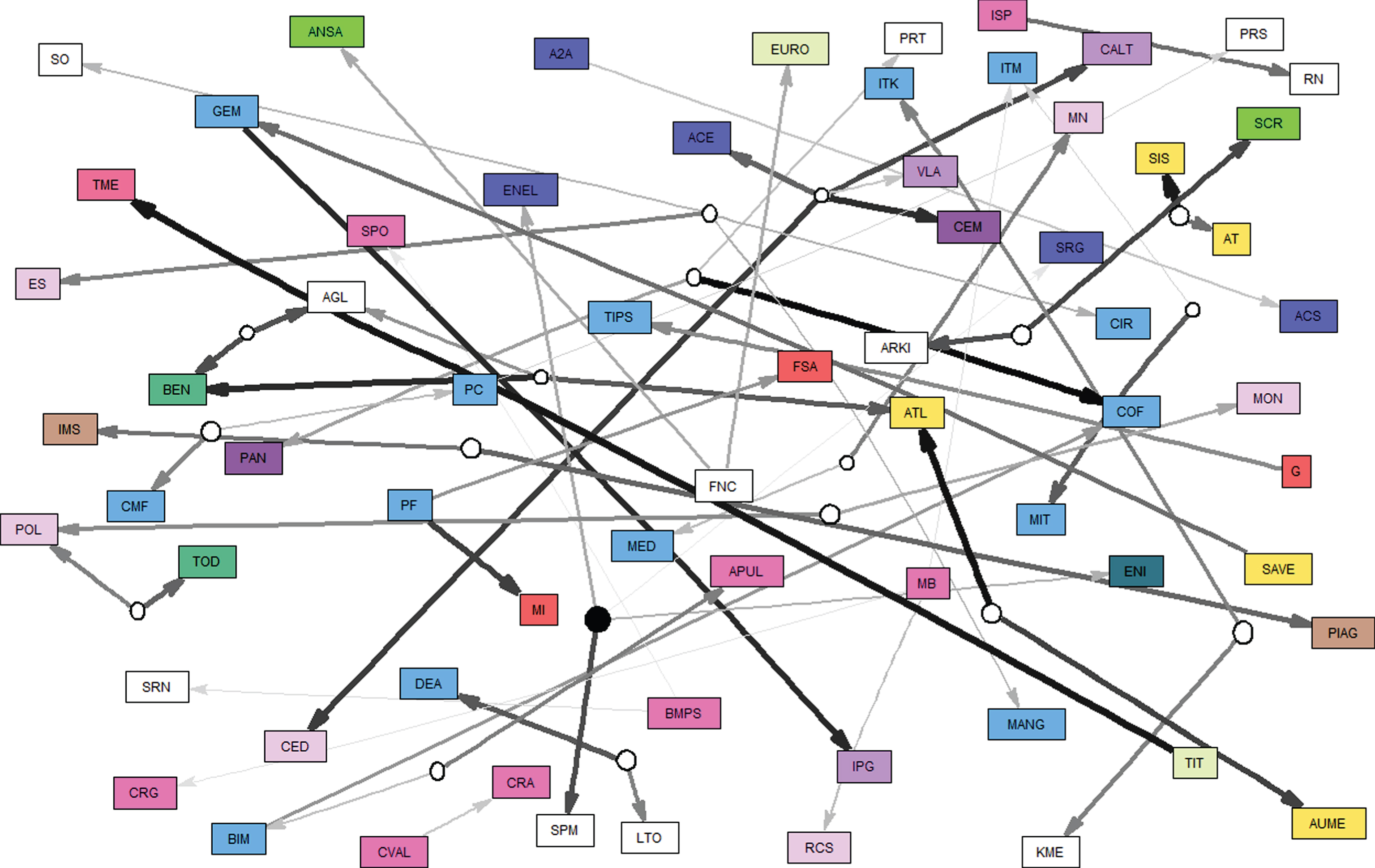
Fig.9
Oriented graph for the 2004 – 2007 average ownerships. Companies are approximately in the same position as in Fig. 2 and companies without owners above 10% are not displayed. Circles are non-quoted companies or people; the black circle is the Italian government. The edge’s thickness represents the ownership percentage.
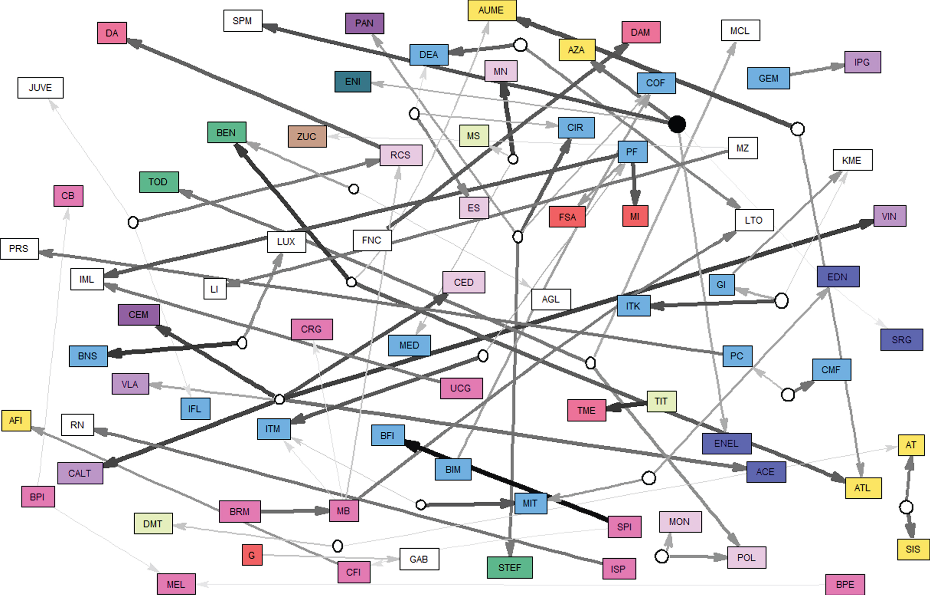
In Fig. 8 the most striking feature is the presence of several strong ownerships for companies far away in the tree, meaning that these ownerships do not influence the MST structure. There are however some ownerships which overlap with the tree’s linkages in Fig. 1: CALT and CEM, SIS and AT, PIAG and IMS, CVAL and CRA, CMF and PC, SPM SRG and ENEL. These ownerships clusters have the feature of involving companies of the same or similar sectors and thus part of the relation is also due to industrial factors. On the other hand, the relation among PF (finance), MI and FSA (insurance) may be due entirely to the ownerships of PF of 40% and 63% respectively.
Switching to Fig. 9 and Fig. 2 we observe that some situations remain the same, in particular for PF with MI and FSA, AT and SIS, CMF and PC, CEM and CALT which gets a direct linkage to VLA. On the other hand, GEM’s ownership of IPG despite being less (46% pre-crises and 68% during the crises) causes reliable linkages between the two companies in the MST. A completely opposite effect is the one between ENEL and SRG, both government-controlled with the same percentage before and during the crises, which are far away before the crises but join together during it. Other linkages influenced by ownership before the crises, which did not exist during the crises, are between MN and MS, GI and ITK, MON and POL, BRM and MB.
In general, we see that both before and after the crises several very large ownerships do not influence the MST construction, as is evident from the many thick arrows which cross Fig. 8 and 9 from one side to the other. There are some exceptions as mentioned before, but they are usually combined with the fact that the involved companies belong to the same or to two similar sectors. Therefore, ownership causes a linkage in the MST when the companies are also in the same sector. As a counterexample, we point out two well-known Italian diversified conglomerates which are in fact very far away in both MSTs. The Benetton family is the controlling shareholder of both Benetton BEN (apparel) and Atlantia ATL (transportation, in particular highways) companies. The De Benedetti family controlled CIR (trading), Stefanel STE (apparel) and Panaria PAN (construction materials) before the crises and CIR, L’Espresso ES (publishing) and Sogefi SO (automobiles) after the crises.
Further inspection of the ownership effects in section 4’s full networks reveals that for the crises networks in Fig. 13 the only relations that correspond to ownerships are between SIS and AT and between MI and FSA, where the involved companies share the same economic activity. Slightly more are the relations in the pre-crises networks of Fig. 15, between SPM and ENI, PC and CMF, PF with MI and FSA. Also, these ones are companies of the same or similar sectors, which suggests that ownership alone does not explain the strong stock return correlation.
Fig.10
Minimum spanning tree for June 2008 – May 2011, considering only the 143 companies present in both periods. Colors represent sectors and edge’s thickness represents reliability.
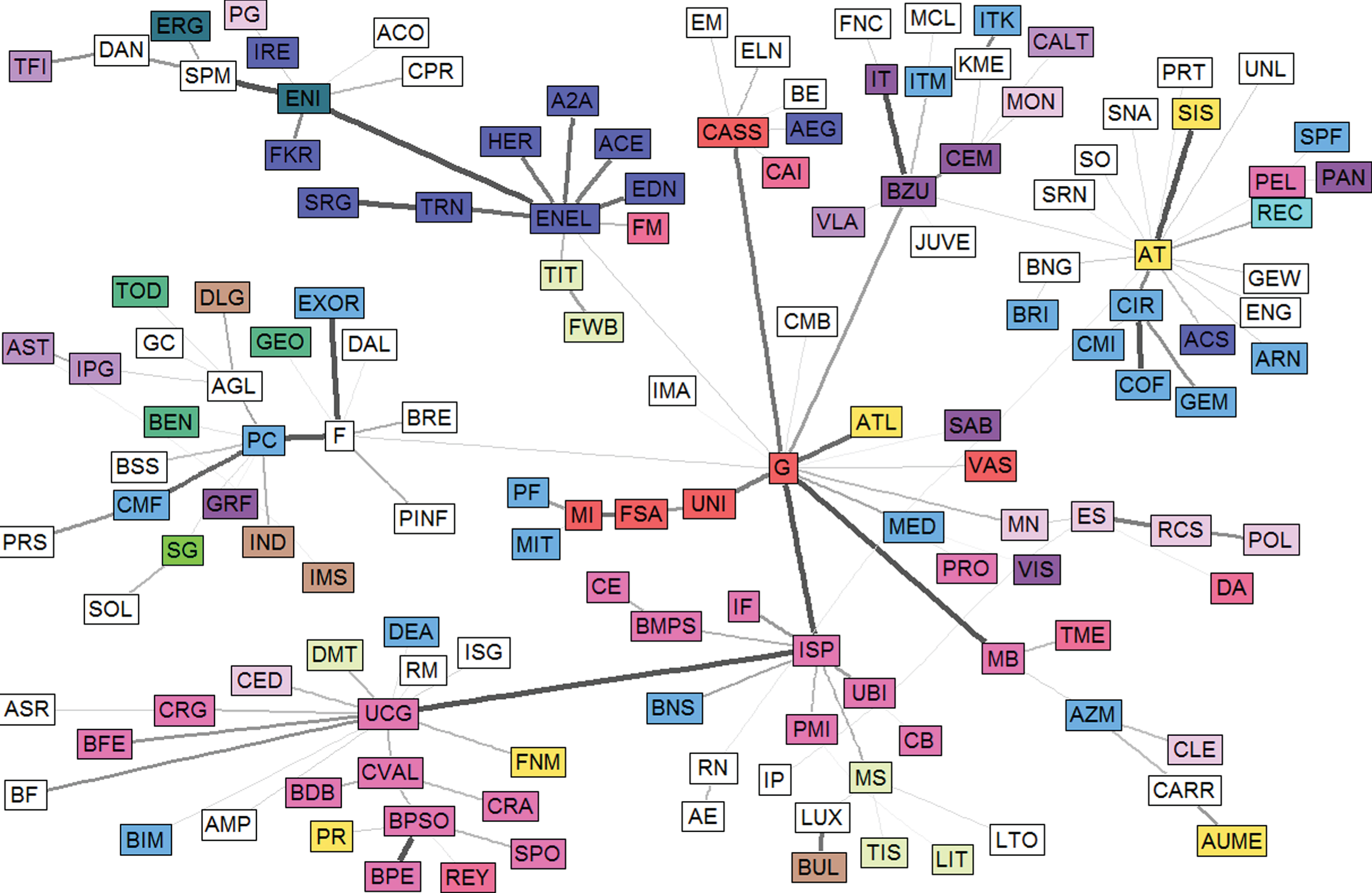
Fig.11
Minimum spanning tree for June 2004 – May 2007, considering only the 143 companies present in both periods. Colors represent sectors and edge’s thickness represents reliability.
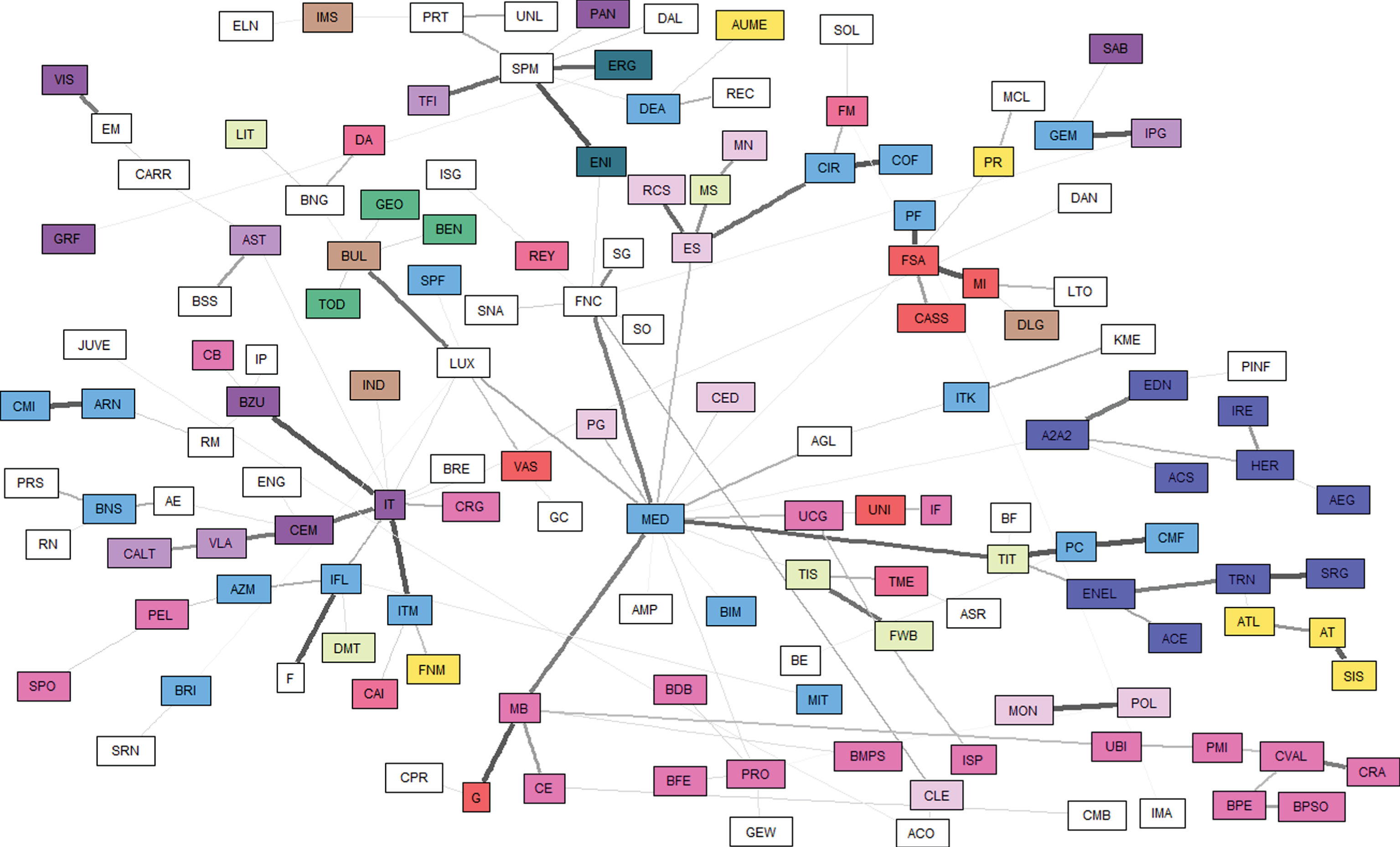
Fig.12
The network for June 2008 – May 2011 with distance threshold 0.775 corresponding to a minimum correlation of 0.7 and to distance 0.3 for Sandoval (2012a). Colors represent sectors and edge’s thickness represents correlation.
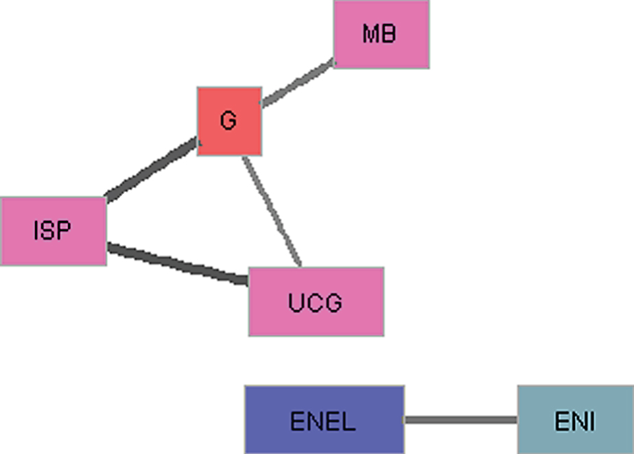
Fig.13
The network for June 2008 – May 2011 with distance threshold 0.894 corresponding to a minimum correlation of 0.6 and to distance 0.4 for Sandoval (2012a). Colors represent sectors and edge’s thickness represents correlation.
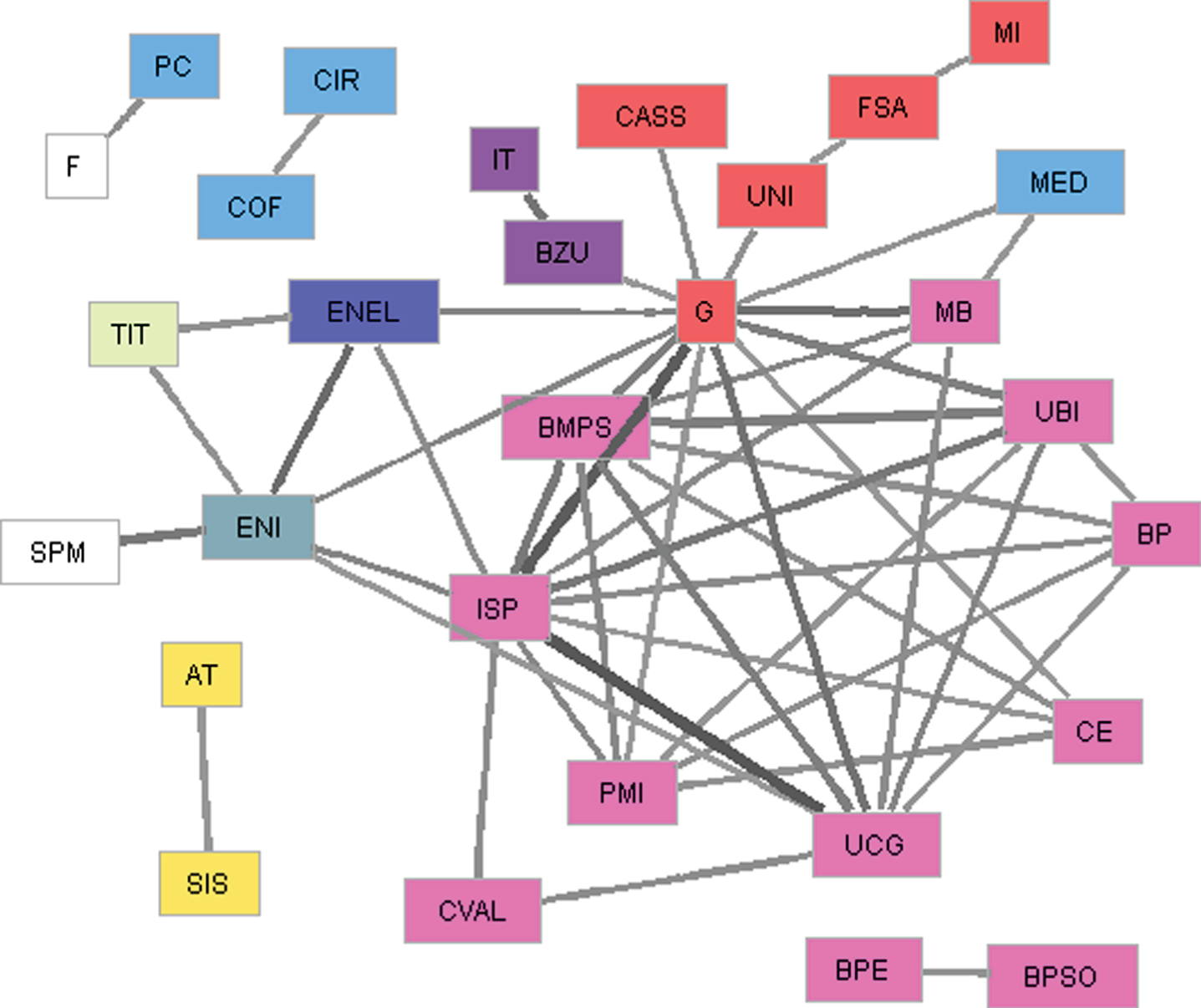
Fig.14
The network for June 2008 – May 2011 with distance threshold 1.0 corresponding to a minimum correlation of 0.5 and to distance 0.5 for Sandoval (2012a). Colors represent sectors and edge’s thickness represents correlation.
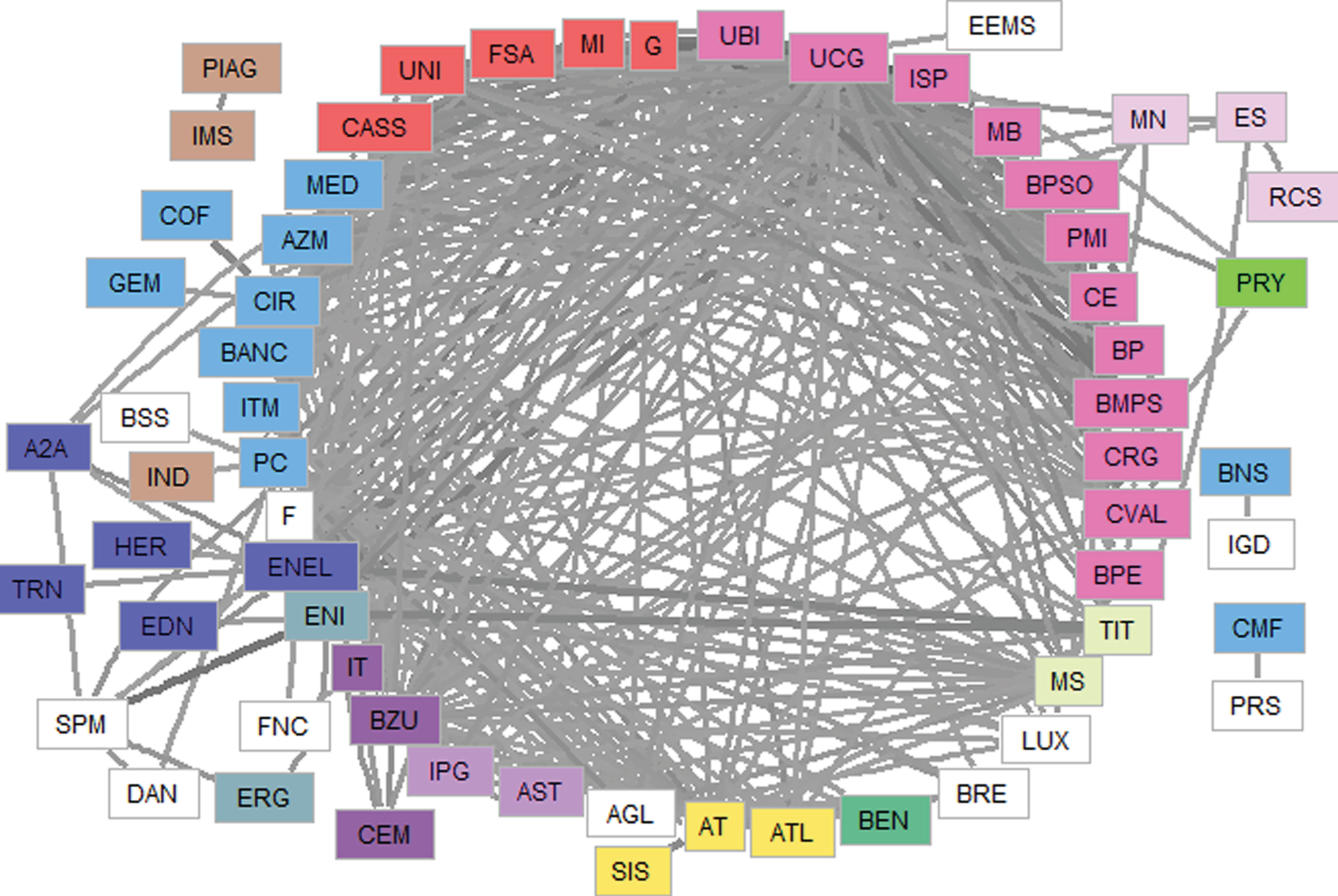
Fig.15
The network for June 2004 – May 2007 with distance threshold 0.894 corresponding to a minimum correlation of 0.6 and to distance 0.4 for Sandoval (2012a) and with distance threshold 1.0 corresponding to a minimum correlation of 0.5 and to distance 0.5 for Sandoval (2012a). Colors represent sectors and edge’s thickness represents correlation.
4.2Survivorship bias
The two samples we use in our empirical analysis do not include the same companies and may influence the MSTs construction. In order to analyze the matched sample bias, we built the MSTs of Fig. 1 and 2, only considering the 143 companies that existed before and during the crises. As usual, companies are kept in the same position to compare these MSTs with the previous ones.
Except for the absence of the 47 non-common companies, the crises MST of Fig. 10 is identical to the one in Fig. 1, with only 3 unreliable linkages that change (IP and ES, AT and RN, IMS and AST). The pre-crises MST of Fig. 11 is also very similar to the one of Fig. 2, but much more unreliable linkages change. Reliable linkages which cause the main hubs remain the same. Only the banking hub in the lower right corner of Fig. 2 is completely taken apart by the removal of SPI and BP2, with the remaining banks however still building linkages to other banks, UCG and mostly MB.
We have also rebuilt the networks of section 4 for the 143 common companies. Apart from the obvious absence of the non-common companies, the crises networks of Fig. 12 remain the same except for the absence of the linkage G UCG whose correlation drops slightly below our threshold, while the ones of Fig. 13 and 14 remain identical. For the pre-crises networks, the networks with only common companies are identical to the ones in Figs. 15–17.
Fig.16
The network for June 2004 – May 2007 with distance threshold 1.095 corresponding to a minimum correlation of 0.4 and to distance 0.6 for Sandoval (2012a). Colors represent sectors and edge’s thickness represents correlation.
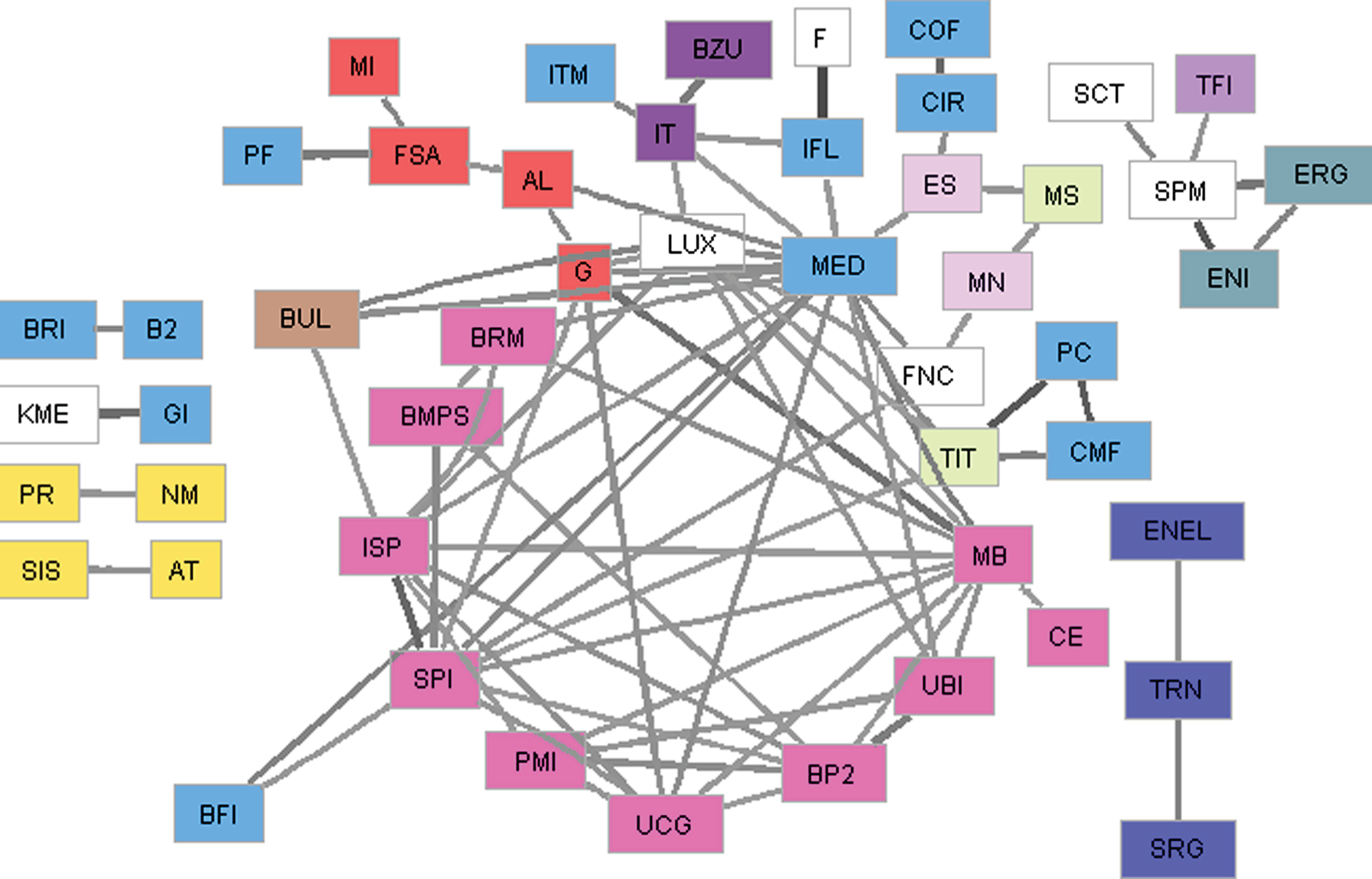
Fig.17
The network for June 2004 – May 2007 with distance threshold 1.183 corresponding to a minimum correlation of 0.3 and to distance 0.7 for Sandoval (2012a). Colors represent sectors and edge’s thickness represents correlation.
We conclude that in general survivorship bias only affects weak linkages, in terms of a low correlation in the network or a small reliability in the MST. This is particularly true for the crises period.
5Network results
Although we introduced the concept of linkage’s reliability, the minimum spanning tree can hide some important correlations in favor of a slightly more important one and in particular never shows cliques. Therefore, following the approach of many authors (Sandoval, 2012a; Onnela et al., 2003a; Nobi et al., 2014; Onnela et al. 2003b), here we illustrate the results for the full network structure. We use a mandatory threshold to filter out edges affected by random correlations as proposed in Section 2, which still leaves too many edges for the graph to be comprehensible in a two-dimensional picture. Thus, we use the same sequence of maximum distance thresholds used by Sandoval (2012a), which also induce minimum correlation thresholds, and display only those edges where the distance is below the threshold.
In Fig. 12 we show the graph for distances below 0.775, which corresponds to the threshold of 0.3 used by Sandoval (2012a) and to correlations above 0.7. Only 5 linkages survive out of 17,955, but they are enough to give us an idea of the core clique of the Italian stock market: Intesa San Paolo (ISP), Unicredit Group (UCG) and Assicurazioni Generali (G), always bound to Mediobanca (MB), something we have already deduced from MST in Fig. 1. The other linkage is the strong bound between ENEL and ENI, the two ex-monopolists of Italian electrical power and natural gas respectively.
Increasing the distance threshold to 0.894, corresponding to a minimum correlation of 0.6 and to Sandoval’s threshold of 0.4, we observe 50 linkages in Fig. 13, building a strongly correlated cluster of banks (pink) together with Assicurazioni Generali (G) that dominates the insurance sector cluster (red) and construction companies (dark purple). The clique ENEL, ENI, Telecom Italia (TIT) is connected to the main companies of the cluster and to the oil extraction machinery company Saipem (SPM). Mediolanum (MED), a financial conglomerate with banking and insurance businesses, is connected to Assicurazioni Generali and Mediobanca (MB), while other dipoles spring into existence.
With a threshold of 1.0 (minimum correlation 0.5) the graph has 365 edges (2% of the total possible edges) and connects 63 companies out of 190. It has become incomprehensible in two dimensions, but it is clear that there exists a large cluster in which banks (pink) and insurance companies (red) held the largest number of linkages, as can be seen from the high density of lines in the upper right part of Fig. 14. The utilities cluster (blue) is strongly connected, the publishing sector (very light purple) is connected as is the construction sector (dark purple), which however is much more integrated in the central cluster.
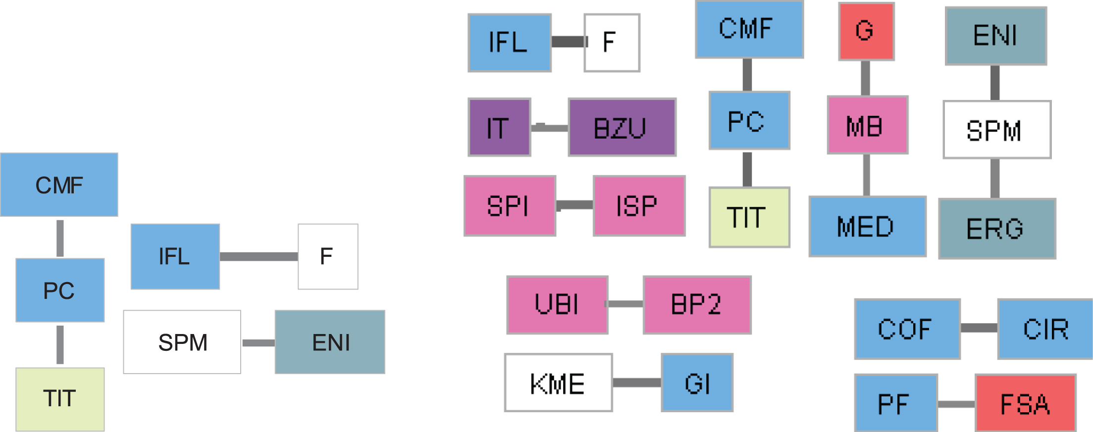
It is interesting to observe the pre-crises network with the same thresholds. Using the first threshold of 0.775, no linkage survives during the pre-crises period. Using the second one, only 4 linkages survive, as can be seen in Fig. 15, which produce no clique but only dipoles and triples among non-banking companies, while the crises graph at this threshold already has a large bank cluster. Increasing it even further to the last step of 1.0, in Fig. 15 we still only observe dipoles and triples with a very small involvement of banks and insurance companies. To see the formation of a bank-dominated cluster as for a crises threshold of 0.894 we have to raise the distance threshold to 1.095, corresponding to a minimum correlation of 0.4 in Fig. 16. However, many disconnected subgraphs exist and to arrive at a situation similar to Fig. 14 we need to further raise the threshold to 1.183 (minimum correlation 0.3) for which, in Fig. 17, we still find the presence of a large number of disconnected dipoles. We can, therefore, conclude that during financial turmoil Italian companies not only increase their correlation but also tend to cluster more with banks and insurance companies rather than building a small subcluster with similar companies, as they did before the crises.
It is also worth noting that the results for theBrazilian market in Sandoval (2012a) are similar to the Italian crises period. Even though they display much shorter minimum distances8, as Sandoval obtains cliques already at our distance threshold of 0.6324 for which we obtain no surviving linkage at all, increasing the threshold to 1, however, he also obtains a large cluster, even though he needs to go one step further to have the same amount of companies in it. On the other hand, the Brazilian market does not display a preference for aggregation around banks and industries, probably also due to the smaller presence of banks (15 against 23) and insurance companies (2 against 6). We conducted further experiments, only considering data for the year 2010, as done by Sandoval (2012a). However, the results are qualitatively similar to those obtained using three years of data with the only difference of more surviving linkages at lower thresholds.
In order to analyze network measures we are going to use a network with a distance threshold of 1.183 to be consistent with Sandoval’s study which applies measures to a network with his distance threshold of 0.7, with both thresholds corresponding to a minimum correlation of 0.3. This results in 4,583 surviving linkages and 158 connected companies. However, when switching to the pre-crises network, this threshold produces a much smaller network with only 502 linkages and 93 connected companies. We do present the results for this network for completeness, but the only conclusion we would be able to draw is its lack of edges. Therefore, we also present the results for the pre-crises period obtained with a second higher threshold of 1.286 (minimum correlation 0.173) which produces 4,528 linkages for 180 connected companies, a situation similar to the crises one.
Analyzing degree’s and eigenvector centrality’s distributions in Fig. 18 we observe no clear difference between the crises network and the pre-crises network with the same amount of linkages, while obviously the results for the pre-crises period with the same threshold as the crises period are completely different due to the smaller amount of linkages. More interesting is the betweenness in Fig. 19 and thek-shell values in Fig. 21. Betweenness centrality for the crises period displays a much smaller betweenness and this can be explained by looking at the k-shell values. The presence of a large number of companies with a high k-shell value means that the crises period has a central cluster, as can be observed in Fig. 14. The crisis cluster is much more populated than the pre-crises cluster. On the other hand, the fact that crises’ k-shell values drop rapidly from the cluster is an indication that the pre-crises period has an outer region of satellite companies which is more connected, while for the crises period these satellite companies have fewer connections with the central cluster. We can thus say that the pre-crises network is more continuously distributed without a net cut between companies in the central cluster and theothers. Strength in Fig. 20 clearly suffers from the fact that the average correlation rises from 13.3% before the crises to 23.3% during the crises, but despite this for low strength nodes we still observe that pre-crises strength is larger, confirming the fact that loosely connected nodes are more connected before the crises.
Fig.18
Distribution of nodes’ degrees and eigenvector centralities for the crises and pre-crises networks with distance threshold 1.183 and for the pre-crises network with distance threshold 1.286.
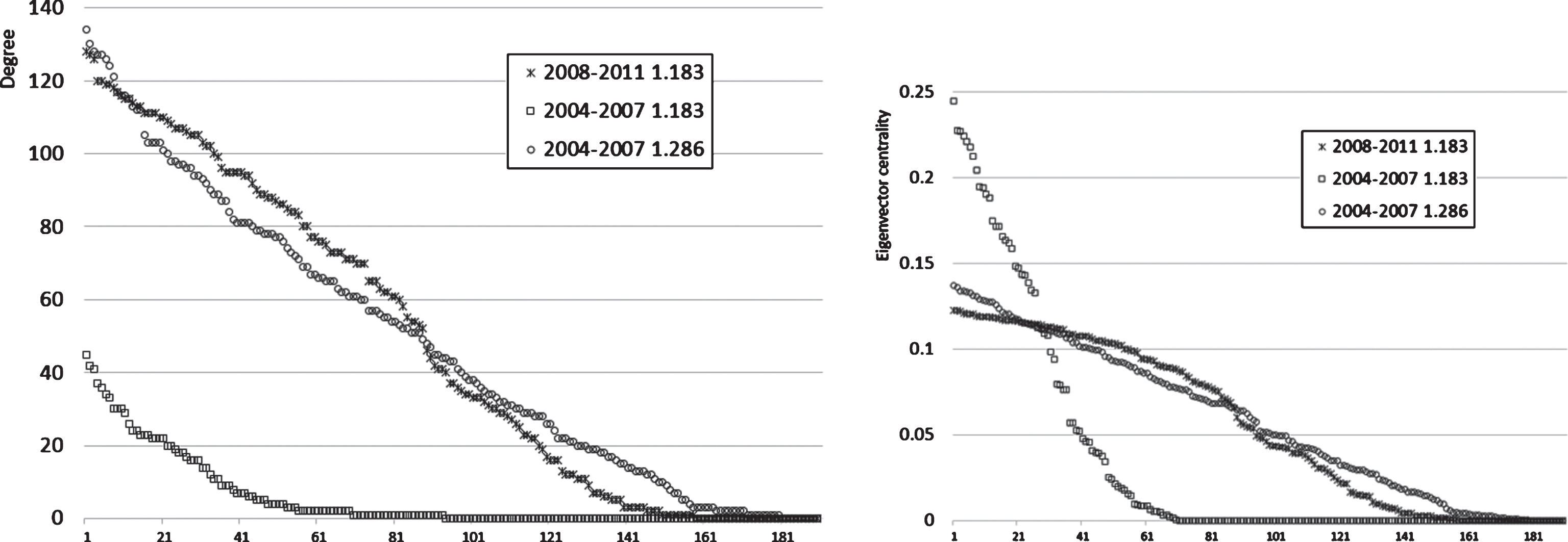
Fig.19
Distribution of nodes’ betweenness centrality for the crises and pre-crises networks with distance threshold 1.183 and for the pre-crises network with distance threshold 1.286. Non-visible nodes have a betweenness of 0.
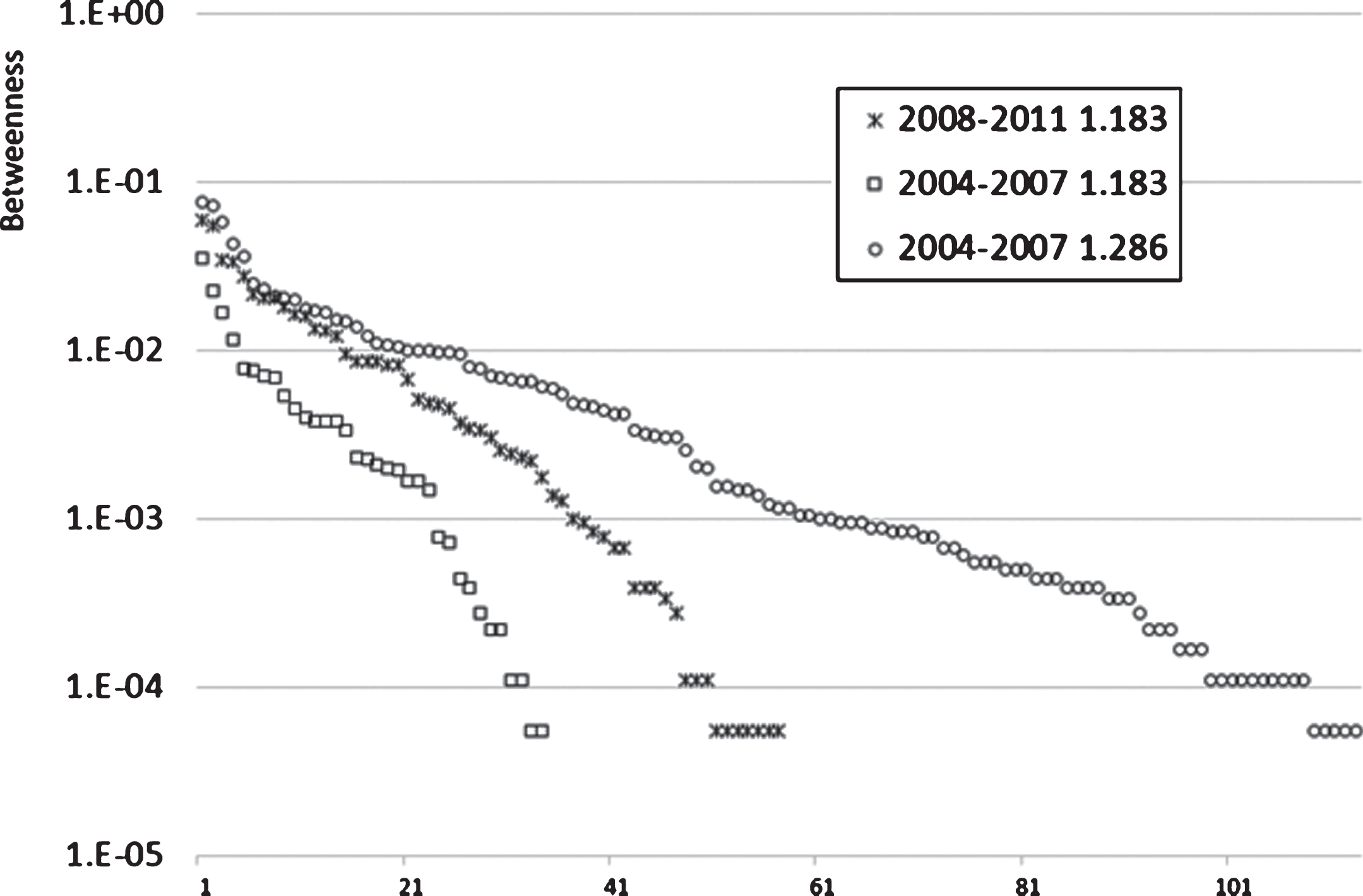
Fig.20
Distribution of nodes’ strength for the crises and pre-crises networks with distance threshold 1.183 and for the pre-crises network with distance threshold 1.286.
To analyze distance and closeness centrality we need to revert to the fully connected network obtained with the threshold 1.3522 explained in Section 2, otherwise disconnected nodes would induce infinity distances which would affect the average distancecalculation. The situation here is obviously dominated by the fact that pre-crises distances are much larger, as evident in Fig. 22.
Fig.21
Distribution of k-shell weighted decomposition’s values for the crises and pre-crises networks with distance threshold 1.183 and for the pre-crises network with distance threshold 1.286. Pre-crises network has 53 nodes with value 47, while crises network has 68 nodes with value 61.
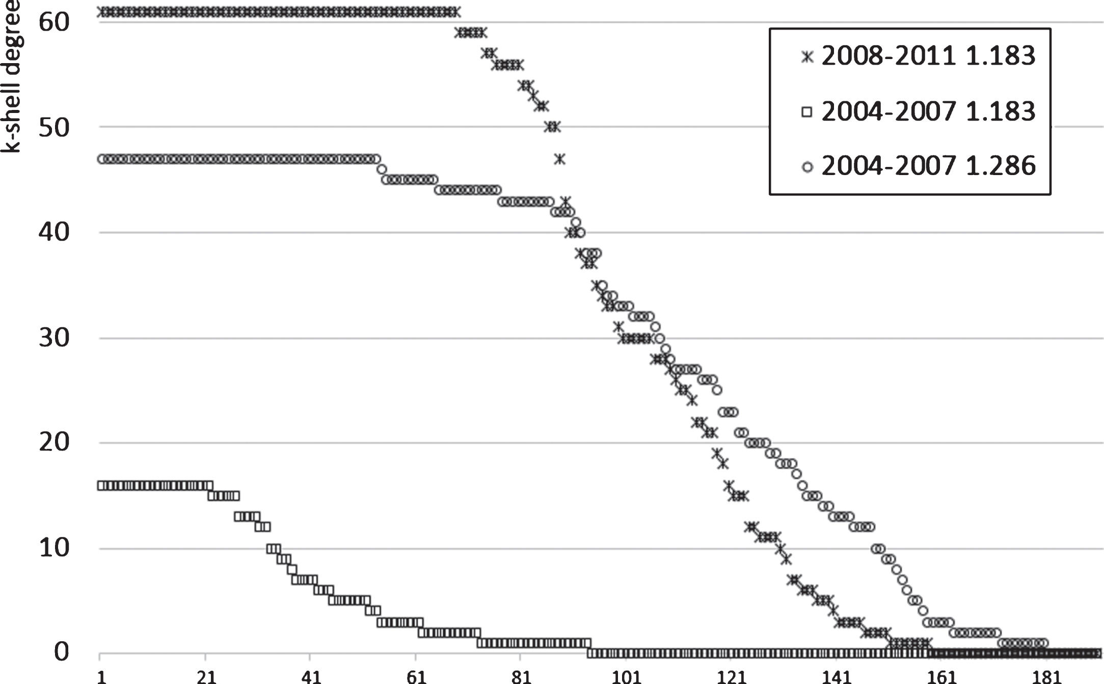
Fig.22
Distribution of nodes’ average distance and closeness centrality for the crises and pre-crises full networks with distance threshold 1.3522.
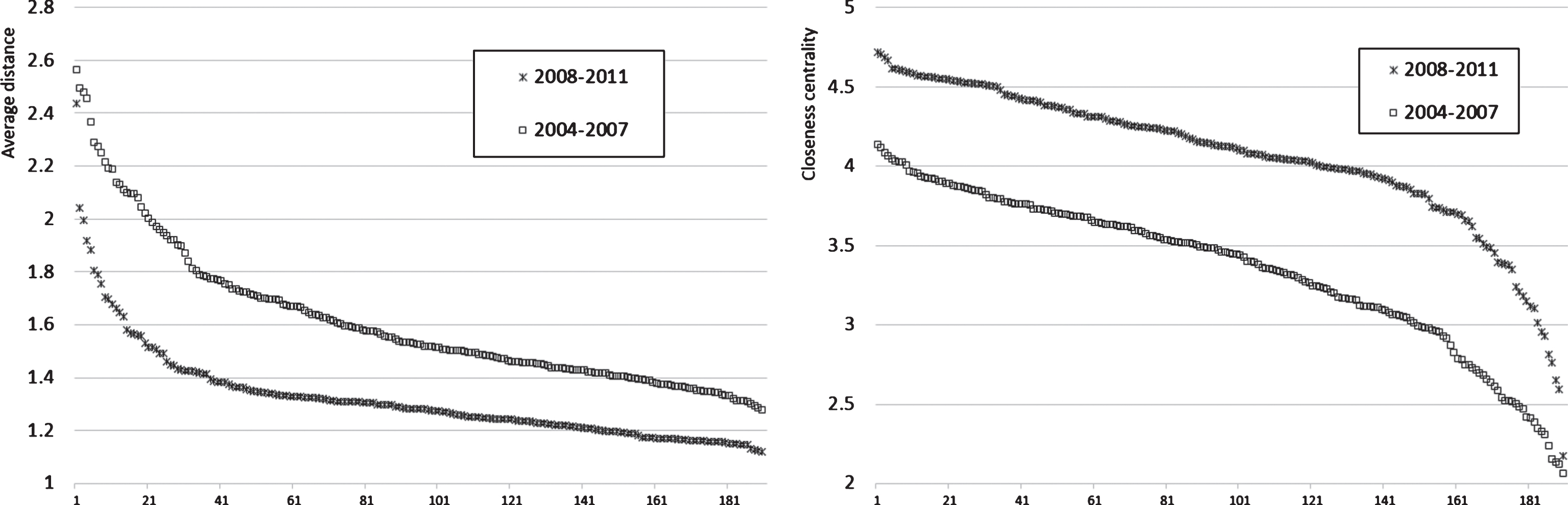
Fig.23
Scatterplot of nodes’ k-shell value versus degree for the crises and pre-crises networks with distance threshold 1.183 and for the pre-crises network with distance threshold 1.286.
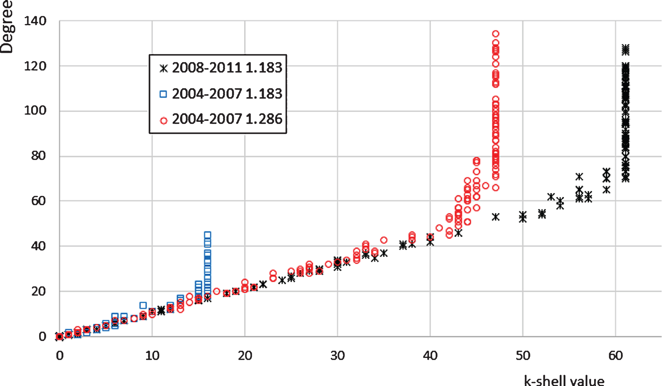
Comparing our result with the Brazilian stock market again we observe a stronger clustering for the Italian network, with 33 nodes (against 23) with degree≥100. The relation between the nodes’ degrees and k-shell value is linear with a final peak, exactly as in Sandoval (2012a), with the major difference that in the Italian case the k-shell limitvalue8 is 61 against 30, meaning that we have twice the amount of companies in the central big cluster. As already highlighted, the Brazilian network looks more similar to the Italian pre-crises period network.
Analyzing the economic sectors in Table 2, we observe that the average intra-sector distance shrinks during the crises for the majority of industries. The few exceptions are the publishing and trading sectors and with a strong contraction for real estate companies. The average intra-sector distance reduction is 15.4%, while the average distance reduction for the network with the same threshold is 5.5%, meaning that companies tend to shorten their distance to similar ones much more than to other companies. Degree by sector, on the other hand, presents a surprise when switching from the pre-crises network 1.286 to the crises network: the banking sector’s degree remains the same which is probably due to the fact that banks are already strongly connected before the crises. Insurance companies, on the other hand, skyrocket their average degree and their average betweenness. We subsequently repeated the calculations excluding Assicurazioni Generali from the insurance sector and we got an average sector degree of 98.6 and betweenness of 0.9. This means that it is not only Assicurazioni Generali but also the entire insurance cluster which jumps at the center of the network. The measure which helps us better understand the dynamics of the network is the k-shell value, which increases for consumer goods, apparel, construction, electrical equipment, automobiles, communication, banking, insurance and real estate, meaning that these sectors are dragged closer to the central big cluster. Some sectors instead, in particular business services, decrease their k-shell and degree average values and they seem to behave in a different way with respect to the rest of the companies.
Table 2
Average distance intra-sector (always for network with threshold 1.3522 to avoid disconnected companies and consequent infinity distances), average degree by sector, average betweenness centrality by sector and average k-shell value by sector, for sectors with at least 5 companies for the network during crises with threshold 1.183 and pre-crises with thresholds 1.183 and 1.286
| June 2008 – May 2011 | June 2004 – May 2007 | ||||||||||||
| Averages by sector | Averages by sector | ||||||||||||
| Sector | Count | Distance intra-sector | Degree | Betweenness centrality | K-shell value | Count | Distance intra-sector | Degree (t = 1.183) | Degree (t = 1.286) | Betweenness (t = 1.183) | Betweenness (t = 1.286) | K-shell value (t = 1.183) | K-shell value (t = 1.286) |
| Printing and Publishing | 8 | 2.3 | 45.3 | 0.1 | 31.4 | 8 | 2.1 | 5.9 | 51.5 | 0.0 | 0.2 | 5.0 | 34.1 |
| Consumer goods | 9 | 2.1 | 39.4 | 0.0 | 31.8 | 7 | 3.7 | 5.1 | 41.0 | 0.0 | 0.3 | 2.3 | 25.6 |
| Apparel | 4 | 1.9 | 65.3 | 0.0 | 47.5 | 6 | 2.9 | 1.7 | 48.7 | 0.0 | 0.2 | 1.7 | 31.0 |
| Construction materials | 9 | 3.5 | 34.7 | 0.2 | 20.4 | 9 | 4.1 | 7.0 | 42.7 | 0.3 | 1.2 | 4.0 | 18.6 |
| Construction | 6 | 2.0 | 63.0 | 0.1 | 42.2 | 6 | 2.4 | 1.7 | 41.3 | 0.1 | 0.1 | 1.5 | 29.2 |
| Machinery | 8 | 2.0 | 48.9 | 0.2 | 30.3 | 7 | 2.4 | 1.4 | 48.4 | 0.1 | 0.5 | 1.1 | 31.9 |
| Electrical equipment | 6 | 3.3 | 25.8 | 0.0 | 22.7 | 4 | 3.9 | 0.0 | 4.0 | 0.0 | 0.0 | 0.0 | 4.0 |
| Automobiles and Trucks | 6 | 2.0 | 79.3 | 0.7 | 53.3 | 5 | 2.0 | 3.6 | 57.0 | 0.0 | 0.0 | 3.0 | 36.8 |
| Utilities | 12 | 2.5 | 44.3 | 0.3 | 31.9 | 13 | 3.0 | 2.5 | 37.1 | 0.1 | 0.2 | 2.0 | 29.2 |
| Communication | 7 | 2.0 | 57.1 | 0.1 | 41.3 | 8 | 2.7 | 4.5 | 46.3 | 0.0 | 0.1 | 3.4 | 34.0 |
| Business Services | 8 | 2.9 | 18.8 | 0.0 | 17.1 | 7 | 3.2 | 0.0 | 35.1 | 0.0 | 0.0 | 0.0 | 25.6 |
| Transportation | 9 | 3.3 | 40.1 | 0.7 | 26.3 | 9 | 3.3 | 0.9 | 35.0 | 0.0 | 0.2 | 1.4 | 25.9 |
| Banking | 23 | 2.1 | 67.9 | 0.5 | 43.8 | 27 | 3.0 | 12.0 | 67.3 | 0.1 | 0.5 | 8.1 | 37.6 |
| Insurance | 6 | 1.9 | 102.0 | 1.3 | 59.2 | 8 | 2.1 | 14.4 | 87.5 | 0.1 | 0.6 | 9.5 | 43.4 |
| Real Estate | 5 | 2.0 | 37.0 | 0.0 | 33.4 | 7 | 3.5 | 0.1 | 28.9 | 0.0 | 0.2 | 0.1 | 22.3 |
| Trading | 22 | 3.4 | 47.4 | 0.2 | 31.3 | 22 | 3.3 | 6.7 | 59.1 | 0.2 | 0.7 | 5.0 | 34.3 |
6Conclusions
Using data for the 190 largest listed Italian companies, we built their network for the two crises period from June 2008 to May 2011. We then compared it to another network, constructed for the pre-crises period June 2004 to May 2007. We followed the methodology first proposed by Mantegna 1999, building a matrix using individual stock return correlations. As a further sample comparison, we selected the Brazilian stock market map during 2010 from Sandoval (2012a). The obtained correlation matrix induces a distance, a minimum spanning tree and a full-connected network which can be pruned with thresholds.
Our empirical analysis highlights the dominance of insurance companies in the Italian stock exchange, which switch from a secondary role in the pre-crises period to a pivotal one during the years of crises. In particular, the large cap company Assicurazioni Generali plays a prominent role in the network map. This was evident from the MST graphs as well as from the lower threshold network graphs, but also its sector’s degree and betweenness centrality increase much more than all the other ones. In the MST, Assicurazioni Generali is a node connecting several star-like hubs, as happens in Sandoval (2012a) for a trading company, while in the full network it is strongly connected with the banking big cluster. Bank stocks are the other main point of difference when comparing results between pre- and post-crises time periods. Their cluster is stronger before and during the crises, but during the crises it absorbs the other companies one after the other, while before the crises there exist several dipoles, triples or cliques of non-banking companies. Majapa and Gossel 2016 found a similar effect in the South African market, where banks originally scattered tend to join together in the crisis MST.
The sectors which remain well clustered beforeand during the crises are publishing, construction, and construction materials. Furthermore, utility and oil & gas stocks show the strongest connections before and during the crises, forming a cluster on its own in the crises MST. This is in contrast to the results in Majapa and Gossel 2016 for South African and in Sandoval (2012a) for Brazil, where multinational companies Sasol and Petrobas, respectively, become the dominant center of their crisis MST, playing the role of Italian banking and insurance industries. The contrasting empirical evidence which emerges between Italy and South Africa and Brazil can be explained by the different role played by oil & gas companies in the three countries. In Italy their main domestic business is distribution, while in South Africa and Brazil it is production (International Energy Agency, 2011). Therefore, as said by Majapa and Gossel 2016, links of oil & gas companies are influenced by foreign economies and they play a mediational influence, which is played by banks and insurance industries in Italy.
Analyzing the graphs, the general contraction of the distances is evident, as found by other authors (Nobi et al., 2014; Heiberger, 2014), but both the MST as well as the network graph change topology in a similar way. The crises MST concentrates its clustering on building several star-like hubs, connected through Assicurazioni Generali, while in the pre-crises MST there were longer chains of companies and Mediolanum played the pivotal role, as already discovered by Brida and Risso 2007 in a similar study with a few Italian companies. The leading role of Mediolanum in the Italian stock market may be related to its indirect ownership of 35% by Silvio Berlusconi, who was prime minister in that period.
While the general increase in correlation coefficients and thus the decrease in distances is exactly what was expected and is evidently due to the decreases in the subsequent rebounds of prices which typically affect the whole market simultaneously during a crisis, the reshaping of the MST is not the same as Nobi et al. (2014) or as the parallel works by Wiliński et al. (2013) and Sienkiewicz et al. (2013). For those works the MST switches from a hierarchy of local stars to a superstar-like tree, whilst the MST of the pre-crises Italian stock market shows a rather diffused tree, without any strongly predominant cluster, and a tree with many local stars around a central company during the crises. In both cases, we do have the rising of a central company, but for the Italian market it plays the role of interconnection among other clusters with a large betweenness, rather than that of a large-degree node. On the other hand, a similar result before and during the crises is obtained by Majapa and Gossel 2016 and we can interpret this as a hint that the transformation MST topology undergoes depends on the pre-crises structure of the market and on the country itself. Further, it must be emphasized that the Italian stock market was first affected by the 2008-2009 financial crisis that started in the USA, and subsequently in 2010 impacted Europe through the sovereign debt crisis that peaked in Italy with a government crisis.
In the network graphs we observe the formation of a large central cluster, as in Nobi et al. (2014) for the Korean market, which during the crises absorbs the companies one after the other leaving the satellite ones loosely connected, while before the crises the central companies were fewer and there was an intermediate shell of companies with many connections among themselves and with the central cluster, as in Heiberger 2014 for the New York stock exchange. This is much more in line with our expectations and with other studies which use networks instead of MST. This discrepancy may be due to the fact that MST tends to hide some strong linkages in favor of slightly better ones and that full networks have a deeper understanding of the situation, even though it is more difficult to represent. We also found an apparent contradiction: on the one side it is very evident from Table 2 that companies shorten the distance to companies of the same sector during the crises much more than to companies outside their sector, but on the other side we observe, in Fig. 17 compared to Fig. 14, during the crises companies abandoning a clustering with a few similar companies in favor of joining the big central cluster. This can be explained by the fact that often pre-crises clusters are not sector clusters but companies with related activities even though they are in a different sector, such as ENI with Saipem (SPM), or by the fact that during the crises it is the entire sector cluster that gets dragged into the central big cluster.
Comparing the Italian network with the Brazilian one (Sandoval, 2012a), however keeping in mind that Sandoval’s analysis does not include the pre-crises period, the Italian pre-crises results show many similarities with the Brazilian crises results, both in terms of numerical distances as well as network topology. The general difference can be attributed to the big differences between the two stock markets, with the Italian one much more dominated by banks, insurance and holding companies. This is confirmed by Tabak et al.’s 2010 study for the Brazilian pre-crises period on a smaller number of companies, which clearly demonstrates the importance of the raw materials sector in the MST, and is further confirmation that transition affects countries in a different way, according to their situation and network pre-crises structure.
Analyzing stock market topology has important implications for portfolio management, such as designing optimal diversification strategies. Practical approaches to portfolio diversification rely on techniques based on size and industry sectors. Approaching a portfolio composition with a market’s network can point out relations among companies which go beyond different sectors and company market capitalization. Alternative clusters can be identified and used to build a portfolio of companies with an effective different price behavior. From the crises tree in Fig. 1 the further information which can be derived is the strong relations of cluster leaders, which means they are not suitable to be considered for good diversification, despite being the representative of their hub. Moreover, the increase in price correlation can be used to confirm a state of crisis and, with further analysis of other crises and countries, to determine the type of crisis and forecast its duration.
Further work could include a much more detailed analysis using sliding time-frames from before the crises up to its core to study linkages survival, as done by Sandoval (2012b and 2013) and Majapa and Gossel 2016, which however would have to cope with the listing, delisting and suspension of some companies which can significantly change the sample characteristics. Using stock market data from Coletti and Murgia 2015, which starts in 1973, we can also study the network’s topology during past decades’ crises like Sandoval and Franca 2012 and Sandoval (2012b) to identify common stock market’s patterns across different economic cycles. Moreover, since MST tends to hide some important relations and does not display cliques while the full network is difficult to visualize, we could analyze the network using other alternative methods, such as planar graph PMFG (Coronnello et al., 2005; Tumminello et al., 2005) or MST with cliques (Onnela et al., 2003a).
Appendices
Appendix
Table 3
The considered companies with the symbol used in this article and the industry sector. The last column indicates whether the company is present only in the crises dataset or in the pre-crises dataset
| Symb | Names | Sector | |
| A2A | A2A | Utilities | |
| AEM | |||
| ACE | ACEA | Utilities | |
| ACO | Acotel Group | Computers | |
| ACS | ACSM Ambiente Gas Acqua Monza | Utilities | |
| AE | AEDES | Real Estate | |
| AEF | AEFFE | Apparel | C |
| AEG | Acegas APS | Utilities | |
| AFI | Aeroporto di Firenze | Transportation | P |
| AGL | Autogrill | Restaurants | |
| AL | Alleanza Assicurazioni | Insurance | P |
| AMP | Amplifon | Wholesale | |
| ANSA | Ansaldo STS | Electronic | C |
| ANTI | Antichi Pellettieri | Consumer | C |
| APUL | Apulia Prontoprestito | Banking | C |
| ARA | Arena | Wholesale | P |
| Roncadin | |||
| ARKI | Arkimedica | Healthcare | C |
| ARN | Alerion | Trading | |
| Fincasa 44 | |||
| ASCO | Ascopiave | Utilities | C |
| ASM | ASM Brescia | Utilities | P |
| ASR | AS Roma | Entertainments | |
| AST | Astaldi | Construction | |
| AT | Autostrada Torino-Milano | Transportation | |
| ATL | Atlantia | Transportation | |
| Autostrade | |||
| AUME | Autostrade Meridionali | Transportation | |
| AZA | Alitalia | Transportation | P |
| AZM | Azimut Holding | Trading | |
| B2 | Bastogi | Trading | P |
| BAN | Basicnet | Retail | C |
| BANC | Banca Generali | Trading | C |
| BDB | Banco di Desio e della Brianza | Banking | |
| BE | Beghelli | Electrical | |
| BEN | Benetton Group | Apparel | |
| BF | Bonifiche Ferraresi | Agriculture | |
| BFE | Banca Finnat | Banking | |
| BFI | Banca Fideuram | Trading | P |
| BIM | Banca Intermobiliare | Trading | |
| BL | Banca Lombarda | Banking | P |
| BMPS | Monte dei Paschi di Siena | Banking | |
| BNG | Buongiorno Vitaminic | Recreation | |
| BNS | Beni Stabili | Trading | |
| BO | Borgosesia | Textiles | C |
| BP | Banco Popolare | Banking | C |
| BP2 | Banco Popolare di Verona e Novara | Banking | P |
| BPE | Banca Popolare dell’Emilia Romagna | Banking | |
| BPI | Banca Popolare di Intra | Banking | P |
| BPSO | Banca Popolare di Sondrio | Banking | |
| BRE | Brembo | Automobile | |
| BRI | Brioschi | Trading | |
| BRM | Capitalia | Banking | P |
| Banca di Roma | |||
| BSS | Biesse | Machinery | |
| BUL | Bulgari | Consumer | |
| BV | Bayerische Vita | Insurance | P |
| Ergo Previdenza | |||
| BZU | Buzzi UNICEM | Constr. materials | |
| CAD | CAD IT | Business services | P |
| CAI | Cairo Communication | Business services | |
| CALT | Caltagirone | Construction | |
| Vianini | |||
| CARR | Carraro | Automobile | |
| CASS | Cattolica Assicurazioni | Insurance | |
| CB | Credito Bergamasco | Banking | |
| CC | Cucirini Cantoni | Textiles | C |
| CDC | CDC | Wholesale | P |
| CE | CREDEM | Banking | |
| CED | Caltagirone Editore | Printing | |
| CEM | Cementir | Constr. materials | |
| CFI | Cassa di Risparmio di Firenze | Banking | P |
| CIR | CIR | Trading | |
| CLE | Class Editori | Printing | |
| CMB | Cembre | Electrical | |
| CMF | CAMFIN | Trading | |
| CMI | ERG Renew | ||
| EnerTAD | Trading | ||
| CMI Cantieri Metallurgici Italiani | |||
| COF | COFIDE | Trading | |
| FINCO | |||
| CPR | Davide Campari | Beer | |
| CRA | Credito Artigiano | Banking | |
| CRG | Banca CARIGE | Banking | |
| CRM | Cremonini | Restaurants | P |
| CVAL | Credito Valtellinese | Banking | |
| DA | DADA | Business services | |
| DAL | Datalogic | Computers | |
| DAM | Datamat | Business services | P |
| DAN | Danieli &C Officine meccaniche | Machinery | |
| DEA | DEA Capital | Trading | |
| CDB Web Tech | |||
| DIA | Diasorin | Pharmaceutical | C |
| DLG | De Longhi | Consumer | |
| DMH | Ducati Motor Holding | Consumer | P |
| DMN | Damiani | Consumer | C |
| DMT | DMT | Telecommunic | |
| EDN | Edison | Utilities | |
| EEMS | EEMS Italia | Electrical | C |
| ELIC | Elica | Electrical | C |
| ELN | El.En. | Measuring equip | |
| EM | EMAK | Machinery | |
| ENEL | ENEL | Utilities | |
| ENG | Engineering Ing Informatica | Computers | |
| ENI | ENI | Oil &Gas | |
| ERG | ERG | Oil &Gas | |
| ES | Gruppo Editoriale L’Espresso | Printing | |
| EURO | Eurotech | Telecommunic | C |
| EUT | Eutelia | ||
| NTS Network Systems | Telecommunic | P | |
| Freedomland | |||
| EXOR | EXOR | Trading | C |
| IFI | |||
| F | FIAT | Automobile | |
| FKR | Falck Renewables | Utilities | |
| Actelios | |||
| FM | Fiera Milano | Business services | |
| FNC | Finmeccanica | Aircraft | |
| FNM | Ferrovie Nord Milano | Transportation | |
| FSA | Fondiaria-SAI | Insurance | |
| FWB | Fastweb | Telecommunic | |
| E.Biscom | |||
| G | Assicurazioni Generali | Insurance | |
| GAB | Gabetti | Real Estate | P |
| GASP | Gas Plus | Oil &Gas | C |
| GC | Gruppo Coin | Retail | |
| Bellini Investimenti | |||
| GEM | Gemina | Trading | |
| GEO | Geox | Apparel | |
| GEW | GEWISS | Electrical | |
| GI | GIM | Trading | P |
| GRF | Granitifiandre | Constr. materials | |
| HER | Hera | Utilities | |
| IF | Banca IFIS | Banking | |
| IFL | IFIL | Trading | P |
| IGD | Immobiliare Grande Distribuzione | Real Estate | C |
| IMA | IMA Industria Macchine Automatiche | Machinery | |
| IML | Immobiliare Lombarda | Real Estate | P |
| IMS | IMMSI | Consumer | |
| IND | Indesit | Consumer | |
| Merloni | |||
| INET | I.NET | Telecommunic | P |
| IP | Interpump Group | Machinery | |
| IPG | Impregilo | ||
| COGEFAR | Construction | ||
| Impresit | |||
| IPI | IPI Attività Immobiliari | Real Estate | P |
| IRC | IRCE | Steel | P |
| IRE | Iren | ||
| Iride | Utilities | ||
| AEM Torino | |||
| ISG | Isagro | Chemicals | |
| ISP | Banca Intesa San Paolo | Banking | |
| IT | Italcementi | Constr. materials | |
| ITH | IT Holding | Apparel | P |
| ITK | INTEK | Trading | |
| ITM | Italmobiliare | Trading | |
| IWA | IW Bank | Banking | C |
| JH | Jolly Hotel | Restaurants | P |
| JUVE | Juventus | Entertainment | |
| KERS | Aión Ren-Kerself | Machinery | C |
| KME | KME | Steel Works | |
| SMI | |||
| KRE | KR Energy | Business services | C |
| LD | La Doria | Food products | P |
| LI | Linificio Canapificio Nazionale | Textiles | P |
| LIT | RETELIT | Telecommunic | |
| LRZ | Landi Renzo | Automobile | C |
| LTO | Lottomatica | Entertainment | |
| LUX | Luxottica | Medical equip | |
| MANG | M&C Management &Capitali | Trading | C |
| MARR | MARR | Restaurants | C |
| MB | Mediobanca | Banking | |
| MBFG | Mariella Burani | Apparel | P |
| MCL | Marcolin | Medical equip | |
| MED | Mediolanum | Trading | |
| MEF | Meridiana Fly | Transportation | C |
| Eurofly | |||
| MEL | Meliorbanca | Banking | P |
| MI | Milano Assicurazioni | Insurance | |
| MIT | Mittel | Trading | |
| MLM | Molmed | Business services | C |
| MN | Mondadori | Printing | |
| MOL | Mutuionline | Banking | C |
| MON | MONRIF Editoriale | Printing | |
| MRT | Mirato | Consumer goods | P |
| MS | Mediaset | Telecommunic | |
| MT | Maire Tecnimont | Construction | C |
| MTV | Mondo TV | Entertainment | P |
| MZ | Marzotto | Textiles | P |
| NICE | Nice | Constr. materials | C |
| NICO | Acquedotto Nicolay | Utilities | P |
| NM | Navigazione Montanari | Transportation | P |
| PAN | Panaria Group | Constr. materials | |
| PAT | Nuova Parmalat | Food | C |
| PC | Pirelli &C | Trading | |
| PEL | Banca Popolare dell’Etruria e del Lazio | Banking | |
| PF | Premafin Finanziaria HP | Trading | |
| PG | Seat Pagine Gialle | Printing | |
| PIAG | Piaggio | Consumer goods | C |
| PIER | Pierrel | Pharmaceutical | C |
| PINF | Pininfarina | Automobile | |
| PIQD | Piquadro | Consumer goods | C |
| PLO | Banca Popolare di Lodi | Banking | P |
| Banca Popolare Italiana | |||
| PMI | Banca Popolare di Milano | Banking | |
| PMS | Permasteelisa | Constr. materials | P |
| POL | Poligrafici Editoriale | Printing | |
| POLF | Poltrona Frau | Consumer goods | C |
| PR | Premuda | Transport | |
| PRI | Prima Industrie | Machinery | C |
| PRO | Banca Profilo | Banking | |
| PRS | Prelios | Real Estate | |
| Pirelli Real Estate | |||
| PRT | Esprinet | Wholesale | |
| PRY | Prysmian | Electronic | C |
| RCS | Holding di Partecipazioni Industriali | Printing | |
| RCS Mediagroup | |||
| RDB | RDB | Constr. materials | C |
| REC | Recordati | Pharmaceutical | |
| REY | Reply | Business services | |
| RIC | Gruppo Ceramiche Ricchetti | Constr. materials | P |
| RM | Reno De Medici | Business supplies | |
| RN | Risanamento Napoli | Real Estate | |
| SAB | SABAF | Constr. materials | |
| SAFI | Safilo Group | Medical equip | C |
| SARA | Saras | Oil &Gas | C |
| SAVE | SAVE Aeroporto di Venezia | Transport | C |
| SCR | SSBT Screen Service | Electronic | C |
| SCT | Socotherm | Fabricated Products | P |
| SERV | Servizi Italia | Business services | C |
| SG | Saes Getters | Electronic | |
| SIS | SIAS | Transport | |
| SNA | Snai | Entertainment | |
| SO | SOGEFI | Automobile | |
| SOL | SOL | Chemicals | |
| SPF | SOPAF | Trading | |
| SPI | San Paolo IMI | Banking | P |
| SPM | SAIPEM | Machinery | |
| SPO | Banca Pop Spoleto | Banking | |
| SRG | Snam Rete Gas | Utilities | |
| SRN | Sorin | Medical equip | |
| STEF | Stefanel | Apparel | P |
| TER | Ternienergia | Electrical | C |
| TFI | Trevi Finanziaria Industriale | Construction | |
| TIPS | TIP | Trading | C |
| TIS | Tiscali | Telecommunic | |
| TIT | Telecom Italia | Telecommunic | |
| Olivetti | |||
| TME | Telecom Italia Media | Business services | |
| Seat | |||
| TOD | Tods | Apparel | |
| TRN | Terna | Utilities | |
| TRV | Trevisan Cometal | Machinery | P |
| TS | Targetti Sankey | Electrical | P |
| TSA | SAT Aeroporto Toscano Galileo Galilei | Transport | C |
| UBI | UBI | Banking | |
| BPU Banche Popolari Unite | |||
| UCG | Unicredit Group | Banking | |
| UNI | Unipol | Insurance | |
| UNL | Uni land | Real Estate | |
| Perlier | |||
| VAS | Vittoria Assicurazioni | Insurance | |
| VIN | Vianini Industria | Construction | P |
| VIS | Greenvision Ambiente | Constr. materials | |
| VLA | Vianini Lavori | Construction | |
| ZIG | Zignago Vetro | Containers | C |
| ZUC | Vincenzo Zucchi | Consumer goods | P |
Notes
1 When a company pays a dividend, its share price artificially drops by approximately the dividend’s amount. When a company increases its capital, the value of the outstanding shares increases thanks to the new fresh money flowing into the company and at the same time it is diluted due to the issue of new shares with dividend and voting rights.
2 The average number of trading days per month is 20.99.
3 In the case of a non-free capital increase, the adjustment factor takes into account not only the market capitalization but also the extra money flown inside the company from the new stockholders’ payments.
4 Sandoval uses as distance dij = 1 - ρij. Since the square root is a monotonic function, both distances induce the same networks provided that a conversion factor is applied to distance thresholds.
5 For sectors with only one or two companies we always use the color white.
6 Sandoval (2012a) defines it as 1/(averagedistance) = n/∑i≠jdij  and calls it inverse closeness centrality.
7 When the voter is not the same as the legal owner, for example in the case of a pledge or an ownerships’ chain, we always take the voter into consideration. Therefore, in the case of a controller with several subsidiaries officially owning the shares, we consider the controller to be the owner.
8 After the necessary conversions, since Sandoval uses d = 1 - ρ Â instead of
9 Our k-shell decomposition uses weighted degrees while Sandoval uses degrees. However, repeating our calculation with the same algorithm used by Sandoval always leads to a limit valueof 61.
References
1 | AIAF, (2014) . Fattori di rettifica. Available at: http://www.aiaf.it/pubblicazioni/fattori-direttifica [Accessed March 6, 2014]. |
2 | Alvarez-Hamelin J.I. , Dall’Asta L. , Barrat A. , Vespignani A. , (2005) . k-core decomposition: A tool for the visualization of large scale networks, arXiv:cs/0504107. |
3 | Antón M. , Polk C. , (2014) . Connected Stocks. The Journal of Finance 69: (3), 1099–1127. doi: 10.1111/jofi.12149 |
4 | Barberis N. , Shleifer A. , (2003) . Style investing. Journal of Financial Economics 68: (2), 161–199. |
5 | Barberis N. , Shleifer A. , Wurgler J. , (2005) . Comovement. Journal of Financial Economics 75: (2), 283–317. |
6 | Bekaert G. , Hodrick R.J. , Zhang X. , (2009) . International Stock Return Comovements. The Journal of Finance 64: (6), 2591–2626. doi: 10.1111/j.1540-6261.2009.01512.x |
7 | Bonanno G. , Caldarelli G. , Lillo F. , Miccichè S. , Vandewalle N. , Mantegna R.N. , (2004) . Networks of equities in financial markets. The European Physical Journal B - Condensed Matter 38: (2), 363–371. doi: 10.1140/epjb/e2004-00129-6 |
8 | Brida J.G. , Matesanz D. , Seijas M.N. , (2016) . Network analysis of returns and volume trading in stock markets: The Euro Stoxx case. Physica A: Statistical Mechanics and its Applications 444: , 751–764.. linkinghub.elsevier.com/retrieve/pii/S0378437115009371 |
9 | Brida J.G. , Risso W.A. , (2010) a. Dynamics and Structure of the 30 Largest North American Companies. Computational Economics 35: (1), 85–99. link.springer.com/10.1007/s10614-009-9187-1 |
10 | Brida J.G. , Risso W.A. , (2007) . Dynamics and Structure of the Main Italian Companies. International Journal of Modern Physics C 18: (11), 1783–1793. |
11 | Brida J.G. , Risso W.A. , (2010) b. Hierarchical structure of the German stock market. Expert Systems with Applications 37: (5), 3846–3852. |
12 | Brida J.G. , Risso W.A. , (2009) . Dynamic and structure of the Italian stock market based on returns and volume trading. Economics Bulletin 29: (3), 2420–2426. |
13 | Coletti P. , Murgia M. , (2015) . Design and Construction of a Historical Financial Database of the Italian Stock Market 1973–2011. Journal of Data and Information Quality 6: (4), 1–23. |
14 | CONSOB, (2016) . CONSOB company data. Available at: http://www.consob.it/mainen/issuers/listed_companies/index.html [Accessed June 20, 2016]. |
15 | Coronnello C. , Tumminello M. , Lillo F. , Miccichè S. , Mantegna R.N. , (2005) . Sector identification in a set of stock return time series traded at the London Stock Exchange. In Acta Physica Polonica B 2653–2679. |
16 | Efron B. , (1979) . Bootstrap methods: Another look at the jackknife. Annals of Statistics 7: (1), 1–26. |
17 | Fama E.F. , (1991) . Efficient Capital Markets: II. The Journal of Finance 46: (5), 1575–1617. doi: 10.1111/j.1540-6261.1991.tb04636.x |
18 | Fama E.F. , (1998) . Market efficiency, long-term returns, and behavioral finance. Journal of Financial Economics 49: (3), 283–306. |
19 | Fama E.F. , French K.R. , (1997) . Industry costs of equity. Journal of Financial Economics 43: (2), 153–193. linkinghub.elsevier.com/retrieve/pii/S0304405X96008963 |
20 | Freeman L.C. , (1977) . A Set of Measures of Centrality Based on Betweenness. Sociometry 40: (1), 35. |
21 | Gałązka M. , (2011) . Characteristics of the Polish Stock Market correlations. International Review of Financial Analysis 20: (1), 1–5. linkinghub.elsevier.com/retrieve/pii/S1057521910000827 |
22 | Gan S.L. , Djauhari M.A. , (2015) . New York Stock Exchange performance: Evidence from the forest of multidimensional minimum spanning trees. Journal of Statistical Mechanics: Theory and Experiment 2015: (12), P12005. |
23 | Garas A. , Schweitzer F. , Havlin S. , (2012) . A k -shell decomposition method for weighted networks. dx. New Journal of Physics 14: (8). doi: 10.1088/1367-2630/14/8/083030 |
24 | Gower J.C. , Ross G.J.S. , (1969) . Trees Minimum Spanning and Single Linkage Cluster Analysis. Journal of the Royal Statistical Society 18: (1), 54–64. |
25 | Grassi R. , (2010) . Vertex centrality as a measure of information flow in Italian Corporate Board Networks. Physica A: Statistical Mechanics and its Applications 389: (12), 2455–2464. linkinghub.elsevier.com/retrieve/pii/S0378437110001408 |
26 | Heiberger R.H. , (2014) . Stock network stability in times of crisis. Physica A: Statistical Mechanics and its Applications 393: , 376–381. |
27 | Heimo T. , Saramäki J. , Onnela J.-P. , Kaski K. , (2007) . Spectral and network methods in the analysis of correlation matrices of stock returns. Physica A: Statistical Mechanics and its Applications 383: (1), 147–151. linkinghub.elsevier.com/retrieve/pii/S0378437107005092. |
28 | Huang W.-Q. , Zhuang X.-T. , Yao S. , (2009) . A network analysis of the Chinese stock market.. dx. Physica A: Statistical Mechanics and its Applications 388: (14), 2956–2964. doi: 10.1016/j.physa.2009.03.028 |
29 | International Energy Agency, (2011) . World Energy Outlook 2011. ISBN 9789264124134. http://www.iea.org/publications/freepublications/publication/WEO2011_WEB.pdf |
30 | Kantar E. , Deviren B. , Keskin M. , (2011) . Hierarchical structure of Turkey’s foreign trade. Physica A: Statistical Mechanics and its Applications 390: (20), 3454–3476. linkinghub.elsevier.com/retrieve/pii/S0378437111003505 |
31 | Khashanah K. , Miao L. , (2011) . Dynamic structure of the US financial systems. Studies in Economics and Finance 28: (4), 321–339. |
32 | Kruskal J.B. , (1956) . On the shortest spanning subtree of a graph and the traveling salesman problem. Proceedings of the American Mathematical Society 7: (1), 48. |
33 | Majapa M. , Gossel S.J. , (2016) . Topology of the South African stock market network across the 2008 financial crisis. Physica A: Statistical Mechanics and its Applications 445: , 35–47. linkinghub.elsevier.com/retrieve/pii/S0378437115009784 |
34 | Mantegna R.N. , (1999) . Hierarchical structure in financial markets. European Physical Journal B 11: , 193–197. |
35 | Mantegna R.N. , Stanley E.H. , (2007) . Introduction to Econophysics: Correlations and Complexity in Finance, Cambridge University Press. |
36 | Newman M.E.J. , (2007) . The Mathematics of Networks. In The New Palgrave Dictionary of Economics. Basingstoke: Nature Publishing Group, 465–470. |
37 | Nobi A. , Maeng S.E. , Ha G.G. , Lee J.W. , (2014) . Effects of global financial crisis on network structure in a local stock market. Physica A: Statistical Mechanics and its Applications 407: , 135–143. linkinghub.elsevier.com/retrieve/pii/S0378437114002945. |
38 | Onnela J.-P. , Chakraborti A. , Kaski K. , Kertész J. , Kanto A. , (2003) a. Asset trees and asset graphs in financial markets. Physica Scripta T106: (1), 48. arxiv.org/abs/cond-mat/0303579 |
39 | Onnela J.-P. , Chakraborti A. , Kaski K. , Kertész J. , (2003) . Dynamic asset trees and Black Monday.. linkinghub.com/retrieve/pii/S. Physica A: Statistical Mechanics and its Applications 324: (1-2), 247–252. linkinghub.elsevier.com/retrieve/pii/S0378437102018824. |
40 | Onnela J.-P. , Chakraborti A. , Kaski K. , Kertész J. , Kanto A. , (2003) b. Dynamics of market correlations: Toaxonmy and portfolio analysis. Physical Review E 68: (5), 056110. doi: 10.1103/PhysRevE.68.056110 |
41 | Piccardi C. , Calatroni L. , Bertoni F. , (2010) . Communities in Italian corporate networks. Physica A: Statistical Mechanics and its Applications 389: (22), 5247–5258. |
42 | Rammal R. , Toulouse G. , Virasoro M.A. , (1986) . Ultrametricity for physicists. Reviews of Modern Physics 58: (3), 765–788. doi: 10.1103/RevModPhys.58.765 |
43 | Sabidussi G. , (1966) . The centrality index of a graph. Psychometrika 31: (4), 581–603. |
44 | Sandoval L. , Franca I.D.P. , (2012) . Correlation of financial markets in times of crisis. Physica A: Statistical Mechanics and its Applications 391: (1-2), 187–208. |
45 | Sandoval L.J. , (2012) a. A Map of the Brazilian Stock Market. Advances in Complex Systems 15: (5), 1–30. arxiv.org/abs/1107.4146 |
46 | Sandoval L.J. , (2013) . Cluster formation and evolution in networks of financial market indices. Algorithmic Finance 2: (1), 3–43. |
47 | Sandoval L.J. , (2012) b. Pruning a minimum spanning tree. Physica A: Statistical Mechanics and its Applications 391: (8), 2678–2711. |
48 | Sienkiewicz A. , Gubiec T. , Kutner R. , Struzik Z.R. , (2013) . Dynamic Structural and Topological Phase Transitions on the Warsaw Stock Exchange: A Phenomenological Approach. Acta Physica Polonica A 123: (3), 615–620. |
49 | Tabak B.M. , Serra T.R. , Cajueiro D.O. , (2010) . Topological properties of stock market networks: The case of BrazilS. Physica A: Statistical Mechanics and its Applications 389: (16), 3240–3249. linkinghub.elsevier.com/retrieve/pii/S0378437110002992. |
50 | Tumminello M. , Aste T. , Di Matteo T. , Mantegna R.N. , (2005) . A tool for filtering information in complex systems. Proceedings of the National Academy of Sciences 102: (30), 10421–10426. |
51 | Tumminello M. , Coronnello C. , Lillo F. , Miccichè S. , Mantegna R.N. , (2007) . Spanning Trees and Bootstrap Reliability Estimation in Correlation-Based Networks. International Journal of Bifurcation and Chaos 17: (07), 2319–2329. doi: 10.1142/S0218127407018415 |
52 | Wiliński M. , Sienkiewicz A. , Gubiec T. , Kutner R. , Struzik Z.R. , (2013) . Structural and topological phase transitions on the German Stock Exchange. Physica A: Statistical Mechanics and its Applications 392: (23), 5963–5973. Http://linkinghub.elsevier.com/retrieve/pii/S037843711300695X. |
53 | Zhuang R. , Hu B. , Ye Z. , (2008) . Minimal spanning tree for Shanghai-Shenzhen 300 stock Index. In IEEE Congress on Evolutionary Computation, CEC 2008 1417–1424. |

