Sparse modeling of volatile financial time&nbsp;series via low-dimensional patterns over&nbsp;learned dictionaries

Tzagkarakis, George; Caicedo-Llano, Juliana; Dionysopoulos, Thomas

doi:10.3233/AF-150051

Sparse modeling of volatile financial time series via low-dimensional patterns over learned dictionaries

Article type: Research Article

Authors: Tzagkarakis, George^{a; *} | Caicedo-Llano, Juliana^b | Dionysopoulos, Thomas^{c; d}

Affiliations: [a] EONOS Investment Technologies, Paris, France | [b] Université d’Evry-Val-d’Essonne, Evry, France | [c] AXIANTA Research, Nicosia, Cyprus | [d] Avenir Finance Investment Managers, Paris, France

Correspondence: [*] Corresponding author: George Tzagkarakis, EONOS Investment Technologies, 12 Rue Mederic, 75017 Paris, France. Fax: +33 148781972; [email protected]

Keywords: Dictionary learning, sparse modeling, financial time series, financial analytics, symbolic representations, transform coding

DOI: 10.3233/AF-150051

Journal: Algorithmic Finance, vol. 4, no. 3-4, pp. 139-158, 2015

Published: 29 December 2015

Get PDF

Abstract

Financial time series usually exhibit non-stationarity and time-varying volatility. Extraction and analysis of complicated patterns, such as trends and transient changes, are at the core of modern financial data analytics. Furthermore, efficient and timely analysis is often hindered by large volumes of raw data, which are supplied and stored nowadays. In this paper, the power of learned dictionaries in adapting accurately to the underlying micro-local structures of time series is exploited to extract sparse patterns, aiming at compactly capturing the meaningful information of volatile financial data. Specifically, our proposed method relies on sparse representations of the original time series in terms of dictionary atoms, which are learned and updated from the available data directly in a rolling-window fashion. In contrast to previous methods, our extracted sparse patterns enable both compact storage and highly accurate reconstruction of the original data. Equally importantly, financial analytics, such as volatility clustering, can be performed on the sparse patterns directly, thus reducing the overall computational cost, without deteriorating accuracy. Experimental evaluation on 12 market indexes reveals a superior performance of our approach against a modified symbolic representation and a well-established wavelet transform-based technique, in terms of information compactness, reconstruction accuracy, and volatility clustering efficiency.

1Introduction

Perceiving and interpreting complicated time-varying phenomena are challenging tasks in several distinct engineering and scientific fields. Such issues become even more demanding in view of the large volumes of raw data that have emerged thanks to the advances of computing technologies. Typical examples include large panel and e-commerce data in finance and marketing, microarray gene expression data in genetics, global temperature data in meteorology, and high-resolution images in biomedical applications, among many others. Knowledge discovery from this data deluge necessitates the extraction of descriptive features in appropriate lower-dimensional spaces, which provide a meaningful, yet compact, representation of the original implicit information to be further employed for executing high-level tasks, such as classification, clustering, pattern discovery and similarity search by content, to name a few.

Focusing on the financial domain, dealing with financial data, which are usually large in size and unstructured, is by no means a non-trivial problem. Technical analysis (Murphy, 1999), which is one of the most commonly used methods for analyzing andpredicting price movements and future market trends, is based on the examination of large volumes of already available past data. To this end, efficient modeling and discovery of informative repetitive patterns in time series ensembles can be applied to understand the underlying behavior within a time series or the relationship among a set of time series and reach a more accurate inference. In the framework of financial data modeling, high-dimensional models, such as vector autoregression (VAR) (Stock and Watson, 2001), have recently gained considerable interest in capturing interdependencies among multiple time series and extracting their inherent structural information. However, standard VAR models are usually constrained in a few tenths of variables, since the number of parameters grows in a quadratic way with the size of the model. In practice, though, financial analysts deal with hundreds of time series, thus making the use of such approaches prohibitive.

Another example concerns the analysis of large stock price data and the need to incorporate cross-sectional effects, since the price of a given stock may depend on various other stocks of the same market, or of distinct markets around the globe. To this end, typical correlation analysis based on ordinary least squares (OLS) estimation can be impractical, since the regression equation may include up to a few thousand stocks. Moreover, in the modern portfolio construction approaches, asset managers rely on the estimation of a large volatility matrix of the assets returns comprising the portfolio to optimize the portfolio’s performance or to manage its risk. However, as it has been shown in Tao et al. (2011), the existing volatility matrix estimators perform poorly and in fact are inconsistent when both the number of assets and the sample sizes go to infinity.

Apart from a computational bottleneck, high dimensionality, which may refer to a large number of time series or a large number of samples, rises two critical issues during data processing, namely, the occurrence of spurious correlations (Fan and Lv, 2010) and the accumulation of noise (Fan and Fan, 2008). Both phenomena can affect unfavorably the systematic computational analysis of our data. Hence, it is important to perform analytics on a faithful representation of the time series, that acts as a close proxy of the raw data in terms of the inherent information content, but which lies in a space of reduced dimensionality enabling a more convenient manipulation.

Several solutions have been proposed to query and index large sets of time series (ref. Zhu and Shasha (2002); Reeves et al. (2009)). Despite their efficiency, these techniques do not support a dedicated storage methodology for compactly and faithfully archiving the entire data series history, as well as for executinginteractive queries on top of the corresponding compact representations. For instance, the system described in Zhu and Shasha (2002) (StatStream) is not effective for correlating noisy data or for preserving significant spikes in data, while the one designed in Reeves et al. (2009) (Cypress) introduces a multi-scale lossy compression of the original data series by maintaining multiple representations of a given time series to be used in distinct queries. However, both techniques could fail in case of financial time series, which usually exhibit quite complicated patterns characterized by non-stationary and transient behavior. On the other hand, our ultimate goal in this work is to design an efficient method for achieving a single compact representation of a given time series, as opposed to the multiple ones produced by Cypress, while still being able to capture the micro-local (spiky) structures, in contrast to StatStream.

A common characteristic of all those time series processing systems is the presence of a dimensionality reduction process, which aims at mitigating the effects of high-dimensional spaces (Jimenez and Langrebe, 1998), such as the limited scalability of algorithms to high-dimensional data, typically due to increased memory and time requirements. Dimensionality reduction techniques can be roughly classified according to their linear or non-linear nature, as well as in terms of a data-adaptive or non data-adaptive behavior.

Traditional linear techniques include principal components analysis (PCA) and factor analysis. However, the main drawback of linear techniques is their inefficiency to adequately handle complex non-linear data. Motivated by this, non-linear techniques for dimensionality reduction have been proposed recently (Lee and Verleysen, 2007). In contrast to their linear counterparts, non-linear methods have the capability to deal with complex data sets. Non-linear methods are further categorized as embedding-based and mapping-based. Embedding-based techniques (Tenenbaum et al., 2000; Roweis and Saul, 2000; Belkin and Niyogi, 2001;Jenkins and Matarić, 2004) model the structure of the data that generates a manifold without providing mapping functions between the observation space and the latent (manifold) space, thus making difficult to map new data into the low-dimensional latent space and vice versa. On the other hand, mapping-based techniques learn appropriate mapping functions either by modeling the non-linear function directly (Schölkopf et al., 1998) or by combining local linear models (Li et al., 2007).

In terms of adaptation capability, non data-adaptive techniques use the same set of parameters for dimensionality reduction regardless of the underlying data. Typical examples include methods which utilize the discrete Fourier transform (DFT) (Agrawal et al., 1993) or a multiresolution decomposition, such as those based on the discrete wavelet transform (DWT) (Chan and Fu, 1999; Kahveci and Singh, 2001). In contrast to DFT, DWT provides increased flexibility by using localized wavelet functions at multiple frequency levels to achieve more compact, yet very accurate, representations of the data. A completely different approach, especially tailored to the analysis of time series, is the piecewise aggregate approximation (PAA) (Yi and Faloutsos, 2000; Chakrabarti et al., 2002), whose simple formation appears to be competitive compared with the more sophisticated transform-based approaches.∥In contrast to the above methods, which represent each data point independently of the rest of the data, data-adaptive techniques account for the underlying data structure and adjust their parameters accordingly. For instance, methods employing a singular value decomposition (SVD) (Wu et al., 1996; Keogh et al., 2001) consider the entire data, thus acting globally and accounting for potential dependencies among them. A conceptually different data-adaptive approach for dimensionality reduction is based on the conversion of time series into sequences of symbols. Symbolic aggregate approximation (SAX) (Lin et al., 2003) is such an example, which employs a PAA representation as an intermediate step between the raw data and the resulting symbolic sequence. SAX-based methods have been utilized efficiently in performing tasks, such as classification, recognition and pattern discovery on distinct types of data (Keogh et al., 2004; Chen et al., 2005; Ferreira et al., 2006; Wijaya et al., 2013).

A major drawback of both the transform-based and symbolic representations is that they may suffer from a significant loss of the inherent information content during the conversion of the original data into highly reduced sets of transform coefficients and symbolic sequences, respectively. In addition, a large amount of historical data is required to ensure that the generated low-dimensional representations will be representative of the range of values that will be observed in the future.

To analyze complex financial time series, and especially to provide fast responses to specific queries, such as classification or indexing, the challenge is to achieve a trade-off between the degree of compactness and the representative capability of the associated low-dimensional representation. For instance, despite their representation accuracy, the majority of the embedding-based methods mentioned above do not scale well with an increasing number of time series or observations, due to their quadratic or cubic complexity in the number of data. As such, they would be inefficient for carrying out classification or indexing tasks over large databases in a timely manner. On the other hand, although transformed-based or symbolic representation methods may achieve inferior performance in terms of representation accuracy in case of complex time series, however, their computational complexity is significantly reduced, and as such they can be very efficient in executing classification or indexing queries in time-constraint applications.

The requirement to attain the trade-off between representation accuracy and high compactness of appropriately extracted patterns from a given time series ensemble can be critical in financial applications. From the one side, we have to maintain a high reconstruction quality of the original time series from the lower-dimensional patterns, in order to achieve accurate inference (e.g., forecasting, classification, indexing). On the other hand, a high compactness of such low-dimensional patterns can be very beneficial towards reducing the storing, archiving, or communication time requirements for huge volumes of financial data generated by the various markets. Motivated by this, the present work introduces a method which compromises the advantages of non-linear techniques in achieving highly accurate, low-dimensional representations of the original data to be further used in higher-level tasks (e.g., classification and indexing), with the advantages of non data-adaptive methods, as mentioned above, in terms of increased scalability and computational efficiency for an increasing number of time series or observations.

More specifically, our proposed method is developed in the framework of sparse representations over learned dictionaries. In the field of signal processing, sparse representations (Bruckstein et al., 2009; Elad, 2010) is one of the most active research areas. The key concept of this theory is that accurate, yet highly compact, representations can be constructed by decomposing signals over elementary atoms chosen from an appropriate dictionary. Sparsity enables faster and simpler processing of the data of interest, since few coefficients reveal all the meaningful information, while also presenting increased robustness to the presence of noise and enhanced reconstruction accuracy from incomplete information.

However, extraction of the sparsest representation is by no means a non-trivial problem. In a transform-based approach, the sparsifying transformation is known and fixed (e.g., DFT or DWT). On the contrary, designing sparsifying dictionaries that best fit our specific data could improve significantly their representative power and achieved sparsity. To this end, dictionary learning has been widely and successfully used in diverse machine learning applications, such as classification, recognition, and image restoration (Aharon et al., 2006). Under this model, each data point is assumed to be expressed as a linear combination of very few atoms, that is, columns of a dictionary, which are jointly learned from a set of training data under strict sparsity constraints. It is also important to highlight that the joint learning process of the dictionary atoms exploits potential correlations among distinct segments of the same time series, or between different time series. This property, which generally improves the representative power and increases the sparsity of the induced representations, is not supported by most of the dimensionality reduction techniques.

Focusing on the case of financial data, given an appropriately learned dictionary and a financial time series we aim at extracting sparse patterns characterized by high representative power, in terms of accurately reconstructing the original data, along with limited storage requirements. Furthermore, we investigate the effectiveness of these sparse patterns in performing clustering based on the volatility estimated directly from them. Volatility clustering was selected as a proper financial analytics to be evaluated due to its importance in quantitative finance. Specifically, accurate volatility clustering enables, among others, the design of more efficient mean reversion models by better understanding the micro-local behavior of a market index.

We also emphasize that the proposed method is not affected by neither the underlying distribution of the original time series, nor their relative magnitudes. These two properties mean that our method is equally efficient for Gaussian and non-Gaussian data, as well as for financial data expressed in local currencies without requiring prior normalization.

1.1Contributions

To summarize, the main contributions of this work are as follows: (i) an adaptive and scalable method is introduced, which exploits the principles of sparse representations over learned dictionaries, for extracting highly representative sparse patterns from financial time series; (ii) the superior performance of the proposed method is illustrated, in terms of information compression through efficient sparse coding, and reconstruction quality of the original time series via an appropriate averaging scheme, when compared with widely used transform-based and symbolic dimensionality reduction techniques tailored to performing queries on time series; (iii) a modified SAX algorithm is introduced by providing additional options for the estimation of more representative breakpoints, which define the associated symbols; (iv) the clustering efficiency of the sparse patterns obtained by our method is demonstrated in terms of clustering distinct segments of financial time series based on their volatility estimated directly from their sparse patterns.

We would also like to note that an exhaustive comparison with all previous state-of-the-art dimensionality reduction techniques is beyond the scope of this paper. Instead, our main goal is to introduce an alternative perspective for performing financial data analytics in an efficient and timely manner. To the best of our knowledge, this is the first time to bridge the theory of sparse representation coding over learned dictionaries with financial data analytics.

The rest of the paper is organized as follows: Section 2 introduces briefly the main concepts of transform-based dimensionality reduction techniques, and describes in detail our modified SAX-based symbolic representation. Section 3 analyzes the building blocks of our proposed method for extracting sparse patterns from financial time series, which comprises of a sparse representation coding step in conjunction with a dictionary learning phase. In Section 4, the performance of the proposed method is evaluated and compared against a transform-based approach and the modified SAX-based method introduced in Section 2, in terms of the achieved compression ratio for storing the low-dimensional representations, the reconstruction quality, and the clustering efficiency based on the estimated volatility. Finally, Section 5 summarizes the main results and gives directions for furtherenhancements.

1.2Notation

In the subsequent analysis, the following notations are adopted. Let x = [x ₁, …, x _N] denote the vectorconsisting of N time series samples. Each sample xi∈ℝ, i = 1, …, N, is the observed value at time t _i, where the set of time instants {t ₁, …, t _N} can be non-uniform (unequally spaced) in the general case. We also note that all the representation methods mentioned in this work will be applied on a rolling window of length w, which slides with a step size equal to s samples across time. Doing so, x _i,w = [x _i-w+1, …, x _i] will denote a window of length w whose ending point is the i-th sample of the original time series x. Furthermore, lowercase letters will denote a scalar, boldface lowercase letters will denote vectors, whereas boldface uppercase letters will denote matrices.

2Transform and symbolic representations of time series

In this section, the main concepts of transform-based dimensionality reduction techniques are introduced briefly, along with a detailed description of our modified SAX-based symbolic representation, which better captures the varying nature of financial data than the standard SAX. As we already noted in Section 1, these two classes of dimensionality reduction techniques were chosen for illustration purposes based on their extensive use in financial technical analysis under storage and temporal limitations for processing specific high-level queries (e.g., indexing (Fu et al., 2004), classification (Lahmiri et al., 2013), and pattern discovery (Ahmad et al., 2004)).

2.1Transform-based time series representations

Transform-based time series representations are powerful signal processing techniques, aiming at mapping efficiently a, usually high-dimensional, time series in an appropriate transform domain, where low-dimensional features can be extracted to represent the meaningful information of the original data. Prominent members of such representations are those techniques which employ the computationally tractable discrete Fourier transform (DFT) and discrete wavelet transform (DWT) (Mallat, 2008).

Specifically, DFT, which maps the time series data from the time domain to the frequency domain, has been extensively used in time series indexing (Rafiei and Mendelzon, 1998) by taking only the first few large-magnitude Fourier coefficients, thus effectively reducing the dimensionality of the representation space and speeding-up the similarity queries. Unlike DFT, which maps the original data from the time domain into the frequency domain, DWT improved the representation accuracy by transforming the data from the time domain into a time-frequency domain. To this end, a multi-scale decomposition of the original time series is performed, which results in an approximation part corresponding to the broad trend of the series, and in several detail parts which represent the localized variations. It is exactly due to its enhanced time-frequency localization property, meaning that most of the time series energy can be represented by only a few high-magnitude wavelet coefficients at multiple scales, that DWT has been shown to achieve superior performance than DFT (e.g., for time series classification) (Wu et al., 2000; Chan et al., 2003).

For convenience, in the rest of the paper we keep a uniform notation for the transform-based time series representations. In particular, if x∈ℝN is a time series with N observations, then

(1)

c=T{x}

where c∈ℝM with, in general, M > N, will denote the set of transform coefficients. Having calculated c, a lower-dimensional subset cs∈ℝS (S ⪡ M) is extracted, which contains a predetermined portion of the total energy of the time series, to represent compactly the original data and perform higher-level tasks, such as clustering and indexing. Since the DWT-based approach will be used as a benchmark for comparison against our proposed technique, we will not go further into its structural details. For a thorough analysis of the DWT’s properties the interested reader is referred to Mallat (2008).

2.2Symbolic time series representations

As mentioned in Section 1, the family of symbolic models has gained recently the interest of the data mining community, due to its simplicity and efficiency when compared with existing dimensionality reduction and data representation methods. A key advantage of symbolic representations, such as SAX, is that they enable the use of many already existing algorithms from the fields of text processing and bioinformatics.

However, financial time series usually present critical or extreme points, which the original SAX method cannot handle. To mitigate the loss of such important points, as well as to account for the underlying trend feature and capture important patterns more accurately, a modified algorithm, the so-called eSAX (Lkhagva et al., 2006), was introduced recently extending the capabilities of the typical SAX representation.

In this section, we introduce a modification of eSAX, which will be used as a benchmark to compare with the performance of sparse representations over learned dictionaries. In particular, our modified eSAX (m-eSAX) algorithm provides additional options for choosing the breakpoints, which determine the interval limits for the associated symbols. More specifically, apart from estimating the breakpoints based on a Gaussian assumption, as is the case with eSAX, for the statistics of the given time series data, we employ three additional options, namely, a) uniform partition of the time series range of values, b) estimation of k q-quantiles of the ordered data, and c) estimation of k q-quantiles of the ordered data by removing repeated values. This modification makes m-eSAX suitable for non-Gaussian distributed data, which is often the case in practice, and also more efficient in extracting specific patterns inherent in financial time series.

The m-eSAX, like any other symbolic representation, aims at representing a contiguous part of a time series as a single symbol, which is selected from a predefined alphabet. Two distinct types of aggregation (segmentation) should be considered, namely, vertical (or temporal) aggregation of the time series values in each window x _i,w, and horizontal aggregation, which changes the granularity of the values a symbol can represent.

Typical operators for vertical aggregation include the average, the sum, the maximum or the minimum value. Following the PAA approach, the average is employed hereafter. Doing so, a given window x _i,w is divided into R equally sized non-overlapping segments of size c =⌊ w/R ⌋, where ⌊a⌋ is the closest integer smaller than a, as follows: xi,w=[gi,w1,…,gi,wR], where gi,wr=[x(i-w+1)+(r-1)c,…,x(i-w+1)+rc-1], r = 1, …, R. Then, for each segment the average is computed by

(2)

μi,wr=Rw∑j=(i−w+1)+(r−1)c(i−w+1)+rc−1xj , r=1,…,R .

In order to capture a more complex data behavior, two additional values, namely, the minimum and the maximum of each segment are also considered. Let mi,wr=min{gi,wr} and Mi,wr=max{gi,wr} be the minimum and maximum values of the r-th segment in the current window, respectively. As a result, the original w-dimensional window x _i,w is mapped to a lower, (3R)-dimensional, representation

(3)

xi,w⟼{(θ11,θ21,θ31),…,(θ1R,θ2R,θ3R)}

where each triplet (θ1r,θ2r,θ3r) is a permutation of the triplet (mi,wr,μi,wr,Mi,wr), for r = 1, …, R. This permutation corresponds to the relative times of occurrence of mi,wr, μi,wr, and Mi,wr. In particular, let [t1,i,wr,…,tc,i,wr] be the time interval corresponding to the r-th segment of the current window. Let also tmi,wrr and tMi,wrr denote the time instants of occurrence of the minimum mi,wr and maximum Mi,wr, respectively, in this time interval. For the average μi,wr we follow the convention that it appears in the middle of the time interval, that is, tμi,wrr=(t1,i,wr+tc,i,wr)/2.

Then, the ordering of the triplet (θ1r,θ2r,θ3r) is determined by the relative position of tmi,wrr, tμi,wrr, and tMi,wrr, as follows:

(4)

(θ1r,θ2r,θ3r) ={(mi,wr,μi,wr,Mi,wr)iftmi,wrr<tμi,wrr<tMi,wrr(Mi,wr,μi,wr,mi,wr)iftMi,wrr<tμi,wrr<tmi,wrr⋮(μi,wr,mi,wr,Mi,wr)otherwise

From (3)-(4) the vertical segmentation of the current window x _i,w consists in forming a sequence of ordered triplets.

A horizontal segmentation comes as the next step, which associates each element of the triplets θjr, j = 1, 2, 3, r = 1, …, R, to a symbol selected from a predetermined alphabet. Horizontal segmentation changes the granularity of the values a symbol from the alphabet can represent. In our m-eSAX, we employ an alphabet consisting of dyadic symbols of variable length by dividing recursively the sub-ranges of real values. In particular, the whole range of values of a given time series is divided into 2^Q intervals, where Q∈ℕ is defined by the user according to the required granularity. In fact, this is equivalent to quantizing the time series data in 2^Q levels, or, equivalently, with Q = log ₂2^Q bits. Table 1 shows examples of dyadic alphabets by varying the value of Q.

Apart from the alphabet, the second component of a horizontal segmentation consists of a set of separator points (or breakpoints). In particular, letA={a1,…,aK} be an alphabet of size K, and B={b1,…,bK-1}, with bi∈ℝ, be a set of breakpoints. Then, each element θir of the triplets defined in (4) is mapped to a symbol aj∈A as follows:

(5)

θir⟼{a1 ifθir≤b1aK ifθir>bK-1aj ifbj-1<θir≤bj(i=1,2,3, r=1,…,R, j=2,…,K-1)

The mapping operators defined by (4) and (5) are applied sequentially on each segment and each sliding window resulting in the final symbolic representation of the original time series x. Figure 1 summarizes the steps of the m-eSAX representation.

The alphabet A and the breakpoints set B constitute the core of the horizontal segmentation. Motivated by Wijaya et al. (2013), we support two additional options to define the breakpoints in m-eSAX. In particular, the breakpoints are generated by using information from the data distribution directly. To this end, two distinct methods are employed to design the set B:

1 Uniform: If m _x = min {x} and M _x = max {x} are the minimum and maximum values of our time series data, then, the range [m _x, M _x] is partitioned uniformly in K equally sized sub-ranges for each of the K symbols.
2 Median: The ordered time series data are divided into K equal-sized subsets (K-quantiles). Then, the breakpoints are defined as the boundary values between adjacent subsets.

In a financial analytics system, data are continuously generated and the processing can be done either when a new value is obtained, or by storing and processing batches of past values. However, all the SAX-based approaches suffer from a possible lack of representation power of the induced symbolic sequence. First, the set of breakpoints B has to be learned on historical data, which should be representative enough for future data. Otherwise, if the range of values assigned to a symbol changes frequently with time, we have to update B, which makes it difficult to implement any algorithm on the generated symbols. This limitation arises naturally in financial applications, where historical data may be unable to represent and describe a typical behavior of the measured phenomenon (e.g., the condition of a global market), which often depends on unpredictable factors.

3Sparse patterns representation of financial time series

The framework of sparse representation coding (SRC) has been gaining a growing interest in the field of signal processing due to its efficiency in revealing the inherent meaningful information content in a significantly lower-dimensional space. In particular, given a signal x∈ℝN, that is, a time series of N observations in our case, and an overcomplete dictionary matrix D=[d1,…,dK]∈ℝN×K, with N < K, then x can be represented as a sparse linear combination of the columns of D. The representation of x over D may be either exact, x = Dα , or approximate, x ≈ Dα with ∥x - Dα ∥ _p ≤ ɛ, where ∥ · ∥ _p denotes the ℓ_p norm. The vector α∈ℝK, which contains the representation coefficients of x, is also known as the sparse code of x. In case of real data, the approximate representation is typically employed, where the deviation is measured in terms of ℓ_p norms for p = 1, 2, and∞.

In the following, our proposed method, hereafter denoted by FTS-SRC (Financial Time Series-Sparse Representation Coding), for representing sparsely, yet highly accurately, volatile financial time series, is analyzed in detail.

3.1Joint optimization for dictionary learning and sparse coding

The overcomplete nature of D, in conjunction with a full rank, yield an infinite number of solutions for the representation problem. Hence, appropriate regularization is required to tackle its ill-posed nature. Motivated by our need to achieve high information compaction, whilst maintaining the inherent structures of volatile financial time series, a sparsity constraint on the representation vector α serves as a means to limit the dimension of the solution space.

To this end, the sparsest representation α is calculated by solving either an exact (P ₀) or an approximate problem (P _0,ɛ) as follows:

(6)

(P0)minα∈ℝK∥α∥0s.t.x=Dα

(7)

(P0,ɛ)minα∈ℝK∥α∥0s.t.∥x-Dα∥2≤ɛ

where ∥ · ∥ ₀ is the ℓ₀ pseudo-norm, which is equal to the number of non-zero elements of a vector.

The majority of sparse representation methods are based on a preliminary assumption that the sparsifying dictionary D is known and fixed. This requires typically a trial-and-error preprocessing step to find the most appropriate dictionary for our data. On the contrary, there is a recent research focus on the proper design of sparsifying dictionaries, which are learned from the available data to better adapt to the underlying data structures, as well as to the sparsity model imposed.

In the following, let X={xj}j=1J, with xj∈ℝN, be a set of training time series. Given X, we seek for a dictionary D, which generates the training series via sparse linear combinations of its atoms (columns). This means that solving the P ₀ problem for each time series x _j yields a corresponding sparse representation α _j, j = 1, …, J. The joint estimation of an adaptive sparsifying dictionary D, along with the associated sparse codes, is performed by solving the following optimization problem:

(8)

minD∈ℝN×K,A∈ℝK×J{∥X-DA∥F2}s.t. ∥αj∥0≤τ, j=1,…,J

where ∥ · ∥ _F denotes the matrix Frobenius norm, A∈ℝK×J is the matrix whose columns are the sparse codes α _j, and τ is a predetermined sparsity level for the α _j’s.

The solution of (8) consists of alternating between a sparse coding step for the estimation of A, and an update step for the dictionary D. For the first step, the dictionary D is considered fixed, and (8) is solved over A. By noting that

(9)

∥X-DA∥F2=∑j=1J∥xj-Dαj∥22

the optimization problem is decoupled into J distinct problems of the form:

(10)

minαj∈ℝK{‖xj−Dαj‖22} s.t. ‖αj‖0≤τ, j=1,…,J .

Each one of these J constrained least-squares optimization problems can be solved efficiently by applying a pursuit algorithm, such as the matching pursuit (MP) (Mallat and Zhang, 1993) or the orthogonal matching pursuit (OMP) (Cai andWang, 2011) among many other existing algorithms. In all these cases, the sparsity level τ affects the maximum number of iterations for the estimation of the, at most, τ non-zero coefficients of each α _j. For the second step, it is assumed that both D and A are fixed, and we seek to update sequentially only one column at a time in the dictionary, d _k (k = 1, …, K), along with the coefficients that correspond to this column, that is, the k-th row of A. The algorithm terminates when a predefined maximum number of iterations has been reached, or when the approximation error falls below a given threshold ɛ.

3.2Extracting sparse micro-local patterns in financial time series

A typical characteristic in most financial data is the presence of micro-local structures in small time windows. Our aim is to represent these structures as accurately as possible by utilizing a minimal amount of information. To this end, we associate the current window of a given time series with its estimated sparse code, thus achieving a mapping between the original dense temporal observations and the space of sparse patterns. These sparse patterns are defined as the estimated sparse codes over the learned dictionary.

The accuracy of the learned dictionary in capturing the significant inherent structures depends also on the representative capability of the training samples. To tackle this issue, given a financial time series x∈ℝN of N observations, it is first divided into two parts, namely, the training set (historical data) xH∈ℝNH and the test set xT∈ℝNT, where N _H + N _T = N. In the following, the dimension of the training set is expressed as a percentage of the total dimension, that is, N _H = δ · N with δ ∈ (0, 1).

In order to better capture the transient micro-local behavior of a volatile financial series, whilst maintaining the inter-dependencies among consecutive time instants, the training data x _H is further partitioned into a set of overlapping sliding windows, x _H;i,w = [x _H, i-w+1, …, x _H, i], of length w using a step size equal to s. The ending point of x _H; i,w is the i-th sample of the training time series x _H. All these windows are then augmented in a single data matrix XH=[xH; w,w|xH; w+s,w|⋯|xH; w+(c˜-1)s,w]∈ℝw×c˜, where c˜=⌊NH-ws+1⌋ is the number of overlapping windows that span x _H.

The corresponding dictionary D _H is learned by solving (8), that is,

(11)

minDH∈ℝw×K, AH∈ℝK×c˜{‖XH−DHAH‖F2} s.t. ‖αH, j‖0≤τ, j=1,…,c˜ .

Having obtained the dictionary for the training set, the associated sparse code α _T, i′ for a window x _T;i′,w in the test set is estimated by solving an MP-like optimization problem (ref. (10)):

(12)

αT, i′=arg{minαT, j′∈ℝK{‖xT;i′,w−DHαT, j′‖22} s.t. ‖αT, j′‖0≤τ} .

By solving (12) and augmenting the resulting sparse codes for all the overlapping windows in the test set x _T, which are also of length w and slide with a step size equal to s, we obtain the sparse representation matrix AT=[αT,1|αT,2|⋯|αT,cˆ]∈ℝK×cˆ, where cˆ=⌊NT-ws+1⌋ is the number of overlapping windows that span the test data x _T. Figure 2 summarizes the steps for learning the dictionary based on a training set, and calculating the sparse codes for both the training and the test data.

The advantage of sparse coding against its symbolic representation counterpart for extracting sparse patterns from volatile time series, is its increased robustness in case of limited training data. As we mentioned before, a major drawback of the symbolic approaches is that the estimated breakpoints, which define the range of values assigned to a symbol, are highly sensitive to the available data. Thus, if the historical (training) data are not representative enough to describe future observations, the resulting symbolic representation yields a degraded approximation, as it will be illustrated by our experimental evaluation. On the contrary, sparse coding over a learned dictionary results in a set of atoms to be used for the representation of a whole window of observations, instead of a few individual values (as is the case with m-eSAX).

Given a highly reduced set of observations, it is more probable to estimate a basis (set of atoms) in which the given time series is approximated accurately, than to estimate a discrete set of transform coefficients or breakpoints, for the transform and symbolic-based methods, respectively, with the capability to represent future distinct observations. As a consequence, the learned dictionary D _H has to be updated much less frequently than the set of breakpoints B, in order to account for the potential variations as new data become available. On the other hand, the predetermined transformation, which plays the role of a dictionary in transform-based methods, remains fixed across time (e.g., wavelet functions in the DWT case).

Concerning the storage requirements, symbolic representations with small-sized alphabets are less demanding, since we only have to store the set B with K - 1 breakpoints (∈ℝ), along with the alphabet A of size K. On the other hand, in case of sparse coding, one has to store a dense matrix DH∈ℝw×K. This is also the case for a transform-based method implemented as a matrix-vector multiplication, such as the DWT, where the associated transform matrix has to be stored. However, in the later case the dictionary or the transform matrix are usually stored on a server with increased memory and processing resources, mitigating their higher size when compared with the necessary information to be stored in case of m-eSAX.

3.3Reconstruction of original volatile series from sparse patterns

Given the learned dictionary D _H and the associated sparse pattern α _j of an arbitrary window x _j,w, which is obtained by solving the optimization problem (12), reconstruction of the original window is simply obtained by

(13)

xˆj,w=DHαj.

Among the several existing algorithms for solving (8), in our proposed approach we relied on the use of K-SVD (Aharon et al., 2006), which is an efficient iterative algorithm that alternates between sparse coding of the training samples based on the current dictionary, and an update step for the dictionary atoms, so as to better fit the data. The dictionary update is performed jointly with an update of the sparse representation coefficients related to it, resulting in accelerated convergence and increased robustness. On the other hand, the sparse pattern of an arbitrary window is obtained by solving (12) using the OMP algorithm, which was shown to achieve a good trade-off between the reconstruction accuracy and the computational cost. We emphasize here that the choice of both the K-SVD and OMP is based on our empirical experimental evaluation, whilst our proposed framework is generic enough to be used with alternative optimization methods depending on the specific requirements of the end-user.

In practice, we are not interested in reconstructing a single individual window, but a series of consecutive overlapping windows as new observations are obtained, and subsequently the original 1-dimensional series. More specifically, without loss of generality, we consider the following case of three overlapping windows, x _w,w, x _w+1,w, and x _w+2,w, of length w and step size equal to s = 1. This means that each window differs from the previous one by a single sample (new observation).

First, each individual window is reconstructed as in (13). Then, the reconstructed samples which belong to more than one windows are averaged to get the final single reconstructed value of each sample. For those samples corresponding to a single window, such as x ₁, the average is the sample by itself. Figure 3 shows this averaging process, which transforms the reconstructed overlapping windows to the original time series data. The same averaging process is also employed for the transform-based approach and the m-eSAX representation to turn the window-by-window reconstruction back to the original 1-dimensional series. On the other hand, if non-overlapping windows are used to scan the original series, then the above averaging scheme is reduced to using the reconstructed sample values by themselves.

4Experimental evaluation

In this section, the performance of sparse pattern extraction over dictionaries learned from volatile financial time series is evaluated in terms of the achieved reconstruction quality of the original data, as well as the amount of information (in bits) required to represent the sparse patterns. Furthermore, the performance of the proposed approach is also evaluated in the framework of volatility clustering by utilizing the sparse patterns directly. Our proposed approach, FTS-SRC, is compared against a typical transform-based representation method by employing the DWT, as well as against m-eSAX.

Our data set consists of a group of 12 developed equity markets (Australia (XP1), Canada (SPTSX), France (CF1), Germany (GX1), Hong Kong (HI1), Japan (TP1), Singapore (QZ1), Spain (IB1), Sweden (OMX), Switzerland (SM1), United Kingdom (Z1), and USA (ES1)). Closing prices at a daily frequency for the main futures indexes of each country have been collected, expressed in local currency, while the covering period is between January 2001 and January 2013. The use of data in local currencies can be advantageous in terms of diversification of international portfolios and does not affect the sparse representation, since the learned dictionary has the capability of automatically adapting to the inherent behavior of each individual country.

During the selected time period, all markets had undergone through various financial crises, such as, the IT-bubble (or dot-com bubble), whose collapse took place by the end of 2001, the global subprimes-debt crisis, whose effects were perceived by the markets in 2007-2008, and the European sovereign crisis in 2010. All crises were followed by a recovery period, which might differ depending on the country and the continent, thus offering a good paradigm to study the adaptability of the learned dictionary in capturing highly diverse micro-local volatile patterns. Table 2 lists the average, volatility, and skewness of the 12 time series in our data set.

Concerning volatility clustering, we adopt the convention that volatility values below 10% are characterized as low, whereas volatility values above 25% are considered to be high. Finally, values ranging in the interval [10 % , 25 %] are characterized as normal. In terms of diversification capabilities for investors, low volatility is related to increased dispersion among the markets or assets, thus offering increased diversification. On the contrary, high volatility usually results in a higher fear factor, which subsequently yields a decrease of the assets trends followed by an increase of their correlation. However, a high correlation between distinct assets is equivalent to lack of diversification, since the assets of interest present similar (correlated) behavior.

4.1Performance metrics

The performance of our proposed method, as well as of the methods against which we compare, is measured in terms of the reconstruction accuracy of the original data based on the corresponding low-dimensional patterns, in conjunction with the information compression ratio between the full-dimensional (original) data and their low-dimensional representations. Concerning the volatility clustering task, its performance is evaluated based on the capability to classify and track the volatility changes in the original data in one of the above three classes (low, normal, high) based solely on the low-dimensional patterns.

Regarding the reconstruction quality of the original financial data, this is measured by means of the root mean squared relative error (RMSRE). In particular, let x and xˆ denote the original and reconstructed time series, respectively. Then, the RMSRE is defined as follows:

(14)

RMSRE(x, x^)=1N∑j=1N(xj−x^jxj)2 .

Concerning the information compression ratio achieved by the corresponding sparse patterns or symbolic sequences, it will be quantified by employing lossless data compression and encoding. In particular, the compression ratio (CR) is defined as follows

(15)

CR=Uncompressed sizeCompressed size

where the uncompressed size and compressed size correspond to the number of bits required to encode the original data and their sparse representations, respectively. Specifically, the elements of both the current data window and its associated sparse pattern are first transformed into a binary stream. Then, this binary stream is compressed in two stages: i) the LZ77 compression algorithm (Ziv and Lempel, 1977) is applied first to replace repeated occurrences of data with references to a single copy of that data existing earlier in the uncompressed stream; ii) Huffman encoding (Cormen et al., 2009) follows as a second step to generate an appropriate codebook, which represents each symbol in the already compressed binary stream, resulting in a prefix code that further compresses the data. For the recovery of the original binary stream, the inverse processes are employed by first applying Huffman decoding followed by LZ77 decompression.

In case of our proposed FTS-SRC method, the achieved compression ratio will depend mainly on the maximum sparsity level, τ, of the patterns, whereas for the transform-based and the symbolic m-eSAX representations, the compression ratios will be controlled by the maximum number of significant (largest magnitude) transform coefficients and the alphabet size, respectively. We emphasize that we do not intend to provide here a sophisticated encoding process of the corresponding representations, but to illustrate the superiority of our proposed approach, when compared with the transform and symbolic-based frameworks, in enabling highly accurate representations of volatile financial series by storing a significantly compressed amount of information. We note that our framework is generic enough and can be used by substituting the compression method adopted here with a more efficient scheme.

4.2Parameter setting for m-eSAX

Our m-eSAX algorithm is applied on the above set of financial time series by varying the window length w _m-eSAX ∈ {30, 60}, the segment size c ∈ {5, 6}, and the alphabet size K _m-eSAX ∈ {64, 128}. The uniform and median horizontal segmentation methods are employed to estimate the breakpoints, along with a dyadic alphabet to generate the symbolic sequence. The choice of the above parameters is based on a requirement to keep a balanced trade-off between the computational complexity and the achieved accuracy of the induced symbolic representations. Notice also that in case of a dyadic alphabet, the step of transforming the low-dimensional representation of the current window into a binary stream is omitted.

4.3Parameter setting for FTS-SRC

In order to achieve a comparable reconstruction quality for a fair comparison with m-eSAX, the window length in our FTS-SRC method varies in w _FTS-SRC ∈ {30, 60}, with a sparsity level τ ∈ {4, 8}. Although a dictionary of increasing size is expected to yield an improved representation performance, for simplicity, we hereafter fix the dictionary size to K _FTS-SRC = 200, and the maximum number of iterations for the K-SVD algorithm to I _max = 100. For both the FTS-SRC and m-eSAX, the number of training samples, which are used for the dictionary learning and the estimation of the breakpoints, respectively, is defined as a percentage of the original time series length N, and is set equal to N _H = δ · N, where δ ∈ {0.5, …, 0.7} and N = 3147.

For the transform-based representation, the DWT is employed. In particular, each window is decomposed to the maximum possible number of scales using the ’db8’ wavelet (e.g., 3 scales for a window length of 128), which was shown to achieve a good trade-off between the reconstruction quality and the compression ratio. We also note that the choice of the optimal wavelet is by its own a separate study, which is beyond the scope of this work. Given the corresponding set of transform coefficients we rely only on those with the highest magnitudes for reconstructing the original time series data. To this end, let K _DWT denote the number of most significant DWT coefficients.In the subsequent evaluation, the value of K _DWT is set by employing scale-dependent thresholds, which are obtained using a wavelet coefficients selection rule based on the Birgé-Massart strategy (Birgé and Massart, 1997). The estimated thresholds, and subsequently the compression ratio, depend on a parameter α. In order to attain comparable compression ratios with our FTS-SRC method, the values of α are chosen from the set {7.5, 8.5}. However, there is no systematic way to define α as a function of the (predetermined) sparsity level for a given wavelet.

4.4Analysis of performance

As a first evaluation of the efficiency of our proposed FTS-SRC method, when compared against a transform-based representation and m-eSAX, we examine the trade-off between the reconstruction quality of the original market indexes and the amount of past information to be used for training the different methods. To this end, the average RMSRE is computed, where the average is taken over all the 12 equity markets, as a function of the percentage of training data. In all the subsequent results, except if otherwise mentioned, the median horizontal segmentation will be used for the m-eSAX representation. Table 3 shows the average RMSRE versus the percentage of training samples for FTS-SRC, m-eSAX, and the transform-based representation by employing the DWT, using the parameter settings described in the previous sections.

Clearly, for the same percentage of training data, FTS-SRC achieves a superior reconstruction quality,when compared against the other two methods. Besides, the performance of FTS-SRC improves as the number of training samples increases, since an increase of historical data enhances the representative power of the learned dictionary for the future observations. On the contrary, the DWT-based approach, as well as the m-eSAX method, present an almost constant behavior. In the case of DWT, this is due to the fact that the wavelet decomposition of the current window does not depend on the past data, thus the number of training samples is irrelevant to the reconstruction quality. On the other hand, for m-eSAX, this can be attributed to the fact that, for the given data set of equity markets, a percentage of 50% of training data is already enough to capture the main underlying structures, without being able to extract more detailed micro-local patterns by increasing the training period.

In Figure 4, the average RMSRE and the average compression ratio are shown for each individual equity index and for the three methods, where the average is taken over the percentages of training samples. First, we note the improved performance of FTS-SRC in reconstructing with high accuracy the original data from the associated sparse patterns, when compared against the symbolic (m-eSAX) and transform-based (DWT) counterparts. Equally importantly, the enhanced reconstruction quality of FTS-SRC comes at significantly higher compression ratios. In contrast to both FTS-SRC and DWT, the m-eSAX approach results in very small compression ratios, while also delivering the highest reconstruction error for most of the equity indexes. The main reason for this behavior is that, although the initial representation of a given data window in terms of triplets, as in (3), is highly compact, however, the size of the alphabet, which maps those triplets to symbols, must be large enough in order to be able to capture the volatile structures of financial time series, thus reducing significantly the overall compression ratio. The enhanced reconstruction performance of FTS-SRC, in conjunction with its high information compressibility, can be very beneficial in financial applications dealing with large data volumes, since the original high-dimensional information can be preserved and processed in a much lower-dimensional space.

Figure 5 shows a typical result for the time series in our data set. In particular, the original market index of Australia (XP1 index) is shown, along with its reconstruction by applying FTS-SRC, m-eSAX, and DWT, for 70% of training data. In accordance with the results shown in the previous figures, FTS-SRC outperforms significantly the m-eSAX approach, whilst DWT follows closely, in terms of approximation accuracy of the original time series. In contrast to FTS-SRC and DWT, which approximate the original data very accurately, m-eSAX introduces artificially high spikes in the reconstructed time series, as it can be seen in the zoomed part of the plot. This is due to the inferior capability of a symbolic representation to capture the behavior of observations which deviate from the boundary (that is, the minimum and maximum) breakpoints. All the values that are lower or higher than the minimum or maximum breakpoint, respectively, are mapped to the minimum or maximum breakpoint irrespectively of how much they deviate from them. On the other hand, although DWT achieves a comparable reconstruction quality with FTS-SRC, it requires the prior choice of a suitable wavelet, which may depend on the specific characteristics of each individual market. However, the advantage of our proposed FTS-SRC is that the estimated dictionary is adapted automatically to the micro-local structures of each market, thus no prior knowledge of the market-wise characteristics is necessary.

The accuracy in reconstruction of these financial time series can be related to the inherent market variation, which is expressed in terms of statistics, such as the volatility and skewness. The 12 analyzed equity markets present volatilities of around 20% and some skewness, as it can be seen in Table 2, whose values are being computed over the whole time period covered by our data set. In the following, we examine the relation between the replication accuracy, as expressed via the RMSRE, and the values of the annualized volatility and skewness for the logarithmic returns of our equity market indexes.

Specifically, let x=[x1,…,xN]∈ℝN be a given time series of prices. Then, the series of logarithmic returns r∈ℝN-1 is defined as

(16)

rt=log(xt)-log(xt-1)t=2,…,N

where x _t is the value of the market variable at the end of time (e.g., day) t, and r _t defines the continuously compounded return during time t (between the end of time t - 1 and the end of time t). It is also noted that, for numerical reasons, we set r ₁ = NaN, since for t = 1 the sample x _t-1 does not exist. Having computed the standard deviation of the returns, σ _r = std (r), the annualized volatility is given by

(17)

σr,annual=σrOs

where O _s denotes the number of open stock market days per year (O _s = 250 for our data set).

To this end, Figure 6 shows the RMSRE (%) versus the annualized volatilities of logarithmic returns for the 12 equity markets and for the three sparse representation methods, where the percentage of training data is fixed at 70%. The common observation for all the three low-dimensional representation methods is that the reconstruction accuracy increases, or equivalently the approximation error decreases, as the annualized volatility of logarithmic returns reduces, following an almost linear dependence. Furthermore, the superiority of our proposed FTS-SRC method against m-eSAX and DWT is revealed once again in achieving highly compact, still very efficient, sparse representations of the original financial data. In addition, the difference in reconstruction performance between FTS-SRC and the other two methods is more prominent especially for higher volatilities, where the time series are, in general, characterized by highly varying micro-local structures. This verifies the capability of FTS-SRC to better adapt to and extract such localized patterns. On the other hand, the improved reconstruction quality, which is achieved for time series with smaller annualized volatility, can be attributed to the fact that a low volatility results in a more representative dictionary for a fixed number of atoms, since the learned dictionary has to capture localized structures of reduced variability.

The effect of skewness on the reconstruction performance is examined in Figure 7, which shows the RMSRE (%) versus the skewness of logarithmic returns for the 12 equity markets. For FTS-SRC an approximately linear relationship exists between RMSRE and skewness, which is not the case for m-eSAX and DWT. In particular, for both the m-eSAX and DWT the reconstruction quality can differ significantly for time series with similar skewness. This is, for instance, the case for SM1 and CF1, as well as for ES1, GX1 and HI1. However, the approximation error is mostly affected by the inherent volatility than the degree of skewness, as it can be concluded by inspecting Figures 6 and 7.

As a last illustration, we evaluate the performance of the three methods in clustering the volatility of the equity market indexes, which is estimated directly from the associated sparse patterns. To this end, Figure 8 shows the moving annualized volatility for the XP1 index in monthly rolling windows with a step size of one week, as it is estimated by employing directly the sparse patterns which are extracted using FTS-SRC, m-eSAX, and DWT. First, we observe that the curve corresponding to FTS-SRC tracks very closely the MAVol curve, which corresponds to the moving annualized volatility values estimated from the original time series. On the other hand, m-eSAX yields both over- and under-estimates of the ground truth volatility, whereas the DWT-based approach results mostly in under-estimated annualized volatility values due to the higher compression of the fine-scale wavelet coefficients via the inherent thresholding process. We note also that these curves represent the volatility over the last 3.5 years in our data set, since the first 70% of the samples are used as a training set.

Finally, we further verify the improved capability of our proposed FTS-SRC method in clustering correctly the windows of low, normal, and high volatility based solely on the extracted sparse patterns. For this purpose, Figure 9 compares the rates of successful volatility clustering in the low (σ _r,annual< 10 %), normal (10% ≤ σ _r,annual ≤ 25 %) or high (σ _r,annual> 25 %) regime between FTS-SRC, m-eSAX and DWT for the 12 equity market indexes. Furthermore, a curve is overlaid on each bar graph, which corresponds to the true number of low, normal, and high volatility windows for each market index, respectively.

Starting from the normal volatility class, which is the most populous among the three, we observe that FTS-SRC yields the highest success rates for all equity indexes, which are also achieved at significantly higher compression ratios when compared with m-eSAX and DWT (ref. Figure 4). On the other hand, DWT delivers the lower success rates, which can be attributed to the fact that a major part of the high-frequency information of the original time series is lost due to the inherent thresholding step, which suppresses many of the fine-scale wavelet coefficients to zero.

This is also the case for the high-volatility class, which is the second most populous among the three. Specifically, FTS-SRC and m-eSAX achieve the highest success rates, whereas the decreased performance of DWT is justified by the loss of high-frequency information as mentioned before. Interestingly, there are cases of indexes (GX1, QZ1, OMX) for which the m-eSAX method achieves slightly improved performance against FTS-SRC. However, this comes at the cost of highly reduced compression ratios in order to preserve the main information content of the original time series (ref. Figure 4).

Lastly, concerning the low-volatility class, FTS-SRC and DWT achieve perfect success rates for all market indexes, except for the Spanish market (IB1 index). From the one hand, for FTS-SRC, this verifies once again the effectiveness of a learned dictionary-based representation to extract the significant micro-local structures. For the DWT-based approach, the high performance is justified by the fact that most of the coarse-scale wavelet coefficients, which represent the low-frequency, thus low-volatile, content of the original time series, are preserved after applying the level-dependent thresholds. In case of IB1, for which no low-volatility windows occur, we observe that only m-eSAX achieves to identify this behavior correctly. On the other hand, FTS-SRC identifies a single window as a low-volatility one, and for this its success rate is set equal to zero. However, this is only a minor issue for FTS-SRC, since the estimated annualized volatility for this single window based on its associated sparse pattern is equal to 9.69%, thus very close to the 10% lower limit. On the contrary, this is not the case for DWT, which wrongly identifies 18 windows in the low-volatility class. Finally, Table 4 summarizes the major advantages and limitations of the three representation methods, FTS-SRC, m-eSAX, and DWT.

5Conclusions and further work

In this work, we introduced a method based on sparse representations over a learned dictionary, in order to extract highly compact sparse patterns, whilst preserving the significant micro-local structures in volatile time series. Furthermore, a modified version of the standard SAX algorithm was also proposed towards enhancing the adaptability of symbolic representations to volatile data.

The efficiency of our proposed sparse coding FTS-SRC method against its symbolic (m-eSAX) and transform-based (DWT) counterparts was highlighted by applying the three distinct methods on a set of volatile equity market indexes. The performance evaluation first revealed the superiority of FTS-SRC in achieving highly accurate reconstructions of the original financial data, while operating at significantly higher compression ratios, when compared with m-eSAX and DWT. Furthermore, we also examined the capability of the three methods in clustering the moving annualized volatility of each market index by relying solely on the associated low-dimensional representations. The experimental results revealed once again that FTS-SRC outperforms the other two alternatives in terms of correctly clustering the distinct windows in the low, normal, and high volatility regimes. On the contrary, m-eSAX was shown to follow the performance of FTS-SRC, but at the cost of significantly reduced compression ratios, whereas DWT was better capable in identifying correctly low and normal volatility data windows rather than high volatility ones.

In addition, a general observation was that the difference in performance, in terms of reconstruction error, between FTS-SRC and the other two methods, increases for increasing annualized volatility and skewness of the corresponding logarithmic returns. This means that FTS-SRC is better capable of adapting to a higher variability of the original data, when compared with m-eSAX and DWT, which is very important when we deal with financial data.

Although in the present work potential correlations among the distinct time series are exploited during the dictionary learning process, however, the presence of common sparse supports between the various time series or data windows, when expressed as linear combinations of the dictionary atoms, is not exploited. Towards this direction, a further enhancement of FTS-SRC can be achieved by incorporating a constraint for extracting jointly (group) sparse supports, which would further improve the interpretation capability of the learned dictionary, while also increasing the degree of sparsity, and subsequently the compression ratio, of the corresponding sparse patterns.

Moreover, the application of FTS-SRC in a real-time financial instrument necessitates the fast update of the learned dictionary, which is the main bottleneck for the overall computational complexity of FTS-SRC. Recent advances in incremental singular value decomposition could be exploited to design an efficient incremental approach for updating the dictionary in a fast online fashion as new observations become available. Finally, the power of sparse representations in embedding the inherent meaningful information in a low-dimensional space will be exploited to perform other tasks of financial interest, such as the discovery of significant motifs and the detection of abnormal events in a given time series, at significantly reduced computational cost.

References

1	Agrawal R. , Faloutsos C. , Swami A. ,(1993) . Efficient similarity search in sequence databases, in Proceedings of th Conference on Foundations of Data Organization and Algorithms, Chicago, Illinois, USA pp. 69–84.
2	Aharon M. , Elad M. , Bruckstein A. ,(2006) . K-SVD: An algorithm for designing overcomplete dictionaries for sparse representation, IEEE Transactions on Signal Processing, 54: (11), 4311–4322.
3	Ahmad S. , Tugba T.-T. , Khurshid A. ,(2004) . Summarizing time series – learning patterns in volatile series, in ‘Intelligent Data Engineering and Automated Learning’, Springer Berlin Heidelberg, pp. 523–532.
4	Belkin M. , Niyogi P. ,(1997) . Laplacian eigenmaps and spectral techniques for embedding and clustering, in Proceedings of Neural Information Processing Systems: Natural and Synthetic, Vancouver, British Columbia, Canada, pp. 585–591.
5	Birgé L. , Massart P. ,(1997) . From model selection to adaptive estimation, Festschrift for Lucien Le Cam, pp. 55–87.
6	Bruckstein A. , Donoho D. , Elad M. ,(2009) . From sparse solutions of systems of equations to sparse modeling of signals and images, SIAM Review 51: 34–81.
7	Cai T. , Wang L. , (2011) . Orthogonal matching pursuit for sparse signal recovery with noise, IEEE Transactions on Information Theory 57: (7), 4680–4688.
8	Chakrabarti K. , Keogh E. , Mehrotra S. , Pazzani M. ,(2002) . Locally adaptive dimensionality reduction for indexing large time series databases, ACM Transactions on Database Systems 27: (2), 188–228.
9	Chan F.K.-P. , Fu A.W.-C. , Yu C.,(2003) . Haar wavelets for efficient similarity search of time-series: With and without time warping, IEEE Transactions on Knowledge and Data Engineering 15: (3), 686–705.
10	Chan K.-P. , Fu A.W.-C. ,(1999) . Efficient time series matching by wavelets, in Proceedings of th IEEE International Conference on Data Engineering, Sydney, NSW, pp. 126–133.
11	Chen J.-S. , Moon Y.-S. , Yeung H.-W. ,(2005) . Palmprint authentication using time series, in Proceedings of th International Conference on Audio- and Video-Based Biometric Person Authentication, Hilton Rye Town, NY, USA, pp. 376–385.
12	Cormen T. , Leiserson C. , Rivest R. , Stein C. ,(2009) . Introduction to Algorithms, 3rd Edition, MIT Press.
13	Elad M. ,(2010) . Sparse and Redundant Representations: From Theory to Applications in Signal and Image Processing, Springer, New York.
14	Fan J. , Fan Y. ,(2008) . High-dimensional classification using features annealed independence rules, The Annals of Statistics 36: (6), 2605–2637.
15	Fan J. , Lv J. ,(2010) . A selective overview of variable selection in high dimensional feature space, Statistica Sinica 20: (1), 101–148.
16	Ferreira P.G. , Azevedo P. , Silva C. , Brito R. ,(2006) . Mining approximate motifs in time series, in Proceedings of th International Conference on Discovery Science, Barcelona, Spain pp. 89–101.
17	Fu T.-C. , Chung F.-L. , Luk R. , Ng C.-M., (2004) . Financial time series indexing based on low resolution clustering, in Proceedings of the ICDM 2004 Workshop on Temporal Data Mining: Algorithms, Theory and Applications, Brighton, UK.
18	Jenkins O.C. , Matarić M. ,(2004) . A spatio-temporal extension to isomap nonlinear dimension reduction, in Proceedings of the st International Conference on Machine Learning, ACM, New York, NY, USA, Banff, Alberta, Canada, p. 56.
19	Jimenez L. , Langrebe D. ,(1998) . Supervised classification in high dimensional space: Geometrical, statistical, and asymptotical properties of multivariate data, IEEE Transactions on Systems, Man, and Cybernetics 28: (1) 39–54.
20	Kahveci T. , Singh A. ,(2001) . Variable length queries for time series data, in Proceedings of th International Conference on Data Engineering, Heidelberg, pp. 273–282.
21	Keogh E. , Chakrabarti K. , Pazzani M. , Mehrotra S. ,(2001) . Dimensionality reduction for fast similarity search in large time series databases, Knowledge and Information Systems3: (3), 263–286.
22	Keogh E. , Chu S. , Hart D. , Pazzani M. ,(2004) . Segmenting time series: A survey and novel approach, Data Mining In Time Series Databases 57: , 1–22.
23	Lahmiri S. , Boukadoum M. , Chartier S. ,(2013) . A supervised classification system of financial data based on wavelet packet and neural networks, International Journal of Strategic Decision Sciences 4: (4), 72–84.
24	Lee J. , Verleysen M. ,(2007) . Nonlinear Dimensionality Reduction, Information Science and Statistics, New York Springer-Verlag.
25	Li R. , Tian T.-P. , Sclaroff S. ,(2007) . Simultaneous learning of nonlinear manifold and dynamical models for high-dimensional time series, in Proceedings of th International Conference on Computer Vision, IEEE, Rio de Janeiro, Brazil, pp. 1–8.
26	Lin J. , Keogh E. , Lonardi S. , Chiu B. ,(2003) . A symbolic representation of time series, with implications for streaming algorithms, in Proceedings of th ACM SIGMOD Workshop on Research Issues in Data Mining and Knowledge Discovery, San Diego, CA, pp. 2–11.
27	Lkhagva B. , Suzuki Y. , Kawagoe K. ,(2006) . Extended SAX: Extension of symbolic aggregate approximation for financial time series data representation, in Proceedings of 22nd International Conference on Data Engineering Workshops, Atlanta, GA, USA.
28	Mallat S. ,(2008) . A wavelet tour of signal processing: The sparse way, Academic Press.
29	Mallat S. , Zhang Z. ,(1993) . Matching pursuits with time-frequency dictionaries, IEEE Transactions on Signal Processing 41: (12) 3397–3415.
30	Murphy J. ,(1999) . Technical Analysis of the Financial Markets: A Comprehensive Guide to Trading Methods and Applications, New York Institute of Finance.
31	Rafiei D. , Mendelzon A. ,(1998) . Efficient retrieval of similar time sequences using DFT, in Proceedings of International Conference of Foundations of Data Organization, Kobe, Japan.
32	Reeves G. , Liu J. , Nath S. , Zhao F. ,(2009) . Managing massive time series streams with multi-scale compressed trickles, in Proceedings of th International Conference on Very Large Data Bases, Lyon, France, pp. 97–108.
33	Roweis S , Saul L , (2000.) . Nonlinear dimensionality reduction by locally linear embedding, Science 209: (2323).
34	Schölkopf B. , Smola A. , Müller K.-R. ,(1998) . Nonlinear component analysis as a kernel eigenvalue problem, Neural Computation 10: (5), 1299–1319.
35	Stock J. , Watson M. ,(2001) . Vector autoregressions, Journal of Economic Perspectives 15: (4)101–115.
36	Tao M. , Wang Y. , Yao Q. , Zou J. ,(2011) . Large volatility matrix inference via combining low-frequency and high-frequency approaches, Journal of the American Statistical Association 106: (495) 1025–1040.
37	Tenenbaum J , Silva V.D , Langford J , (2000) . A global geometric framework for nonlinear dimensionality reduction, Science 290: (5500), 2319–2323.
38	Wijaya T.K. , Eberle J. , Aberer K. ,(2013) . Symbolic representation of smart meter data, in Proceedings of the Joint EDBT/ICDT Workshops, Genoa, Italy, pp. 242–248.
39	Wu D. , Singh A. , Agrawal D. , Abbadi A.E. , Smith T. ,(1996) . Efficient retrieval for browsing large image databases, in Proceedings of th International Conference on Information and Knowledge Management, Rockville, MD, pp. 11–18.
40	Wu Y.-L. , Agrawal D. , Abbadi A.E. ,(2000) . A comparison of DFT and DWT based similarity search in time-series databases, in Proceedings of the 9th International Conference on Information and Knowledge Management, ACM, McLean, Virginia, USA.
41	Yi B.K. , Faloutsos C. ,(2000) . Fast time sequence indexing for arbitrary Lp norms, in Proceedings of th International Conference on Very Large Data Bases, Cairo, Egypt, pp. 385–394.
42	Zhu Y. , Shasha D. ,(2002) . StatStream: statistical monitoring of thousands of data streams in real time, in Proceedings of th International Conference on Very Large Data Bases, Hong Kong, China, pp. 358–369.
43	Ziv J. , Lempel A. ,(1997) . A universal algorithm for sequential data compression, IEEE Transactions on Information Theory, 23: (3) 337–343.

Figures and Tables

Fig.1

Flow diagram of the m-eSAX symbolic representation.

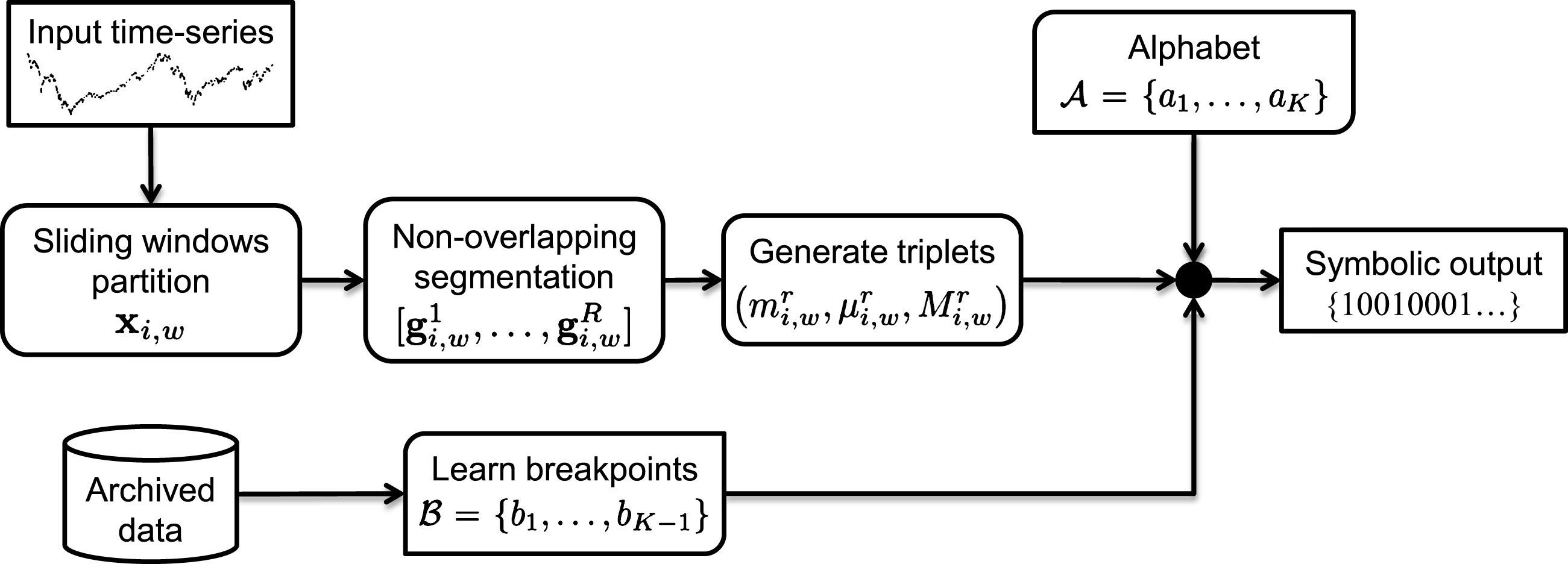
Fig.2

Flow diagram of sparse representation coding of a given time series based on a learned dictionary.

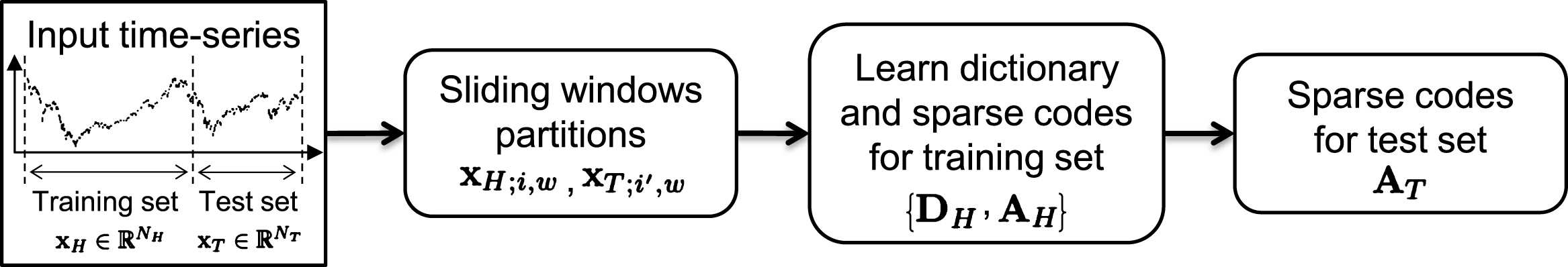
Fig.3

Averaging of reconstructed overlapping windows to obtain original time series.

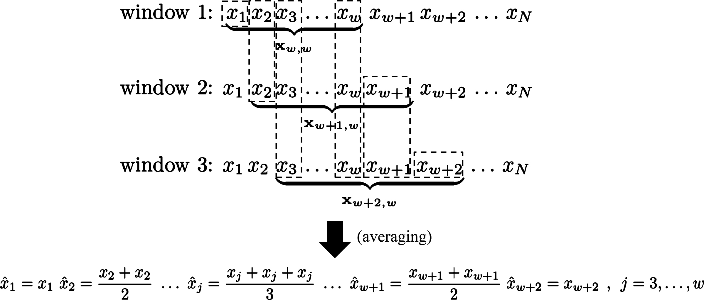
Fig.4

Average RMSRE and average Compression Ratio for each equity index for FTS-SRC, m-eSAX, and DWT-based representations (average is taken over the percentage of training samples).

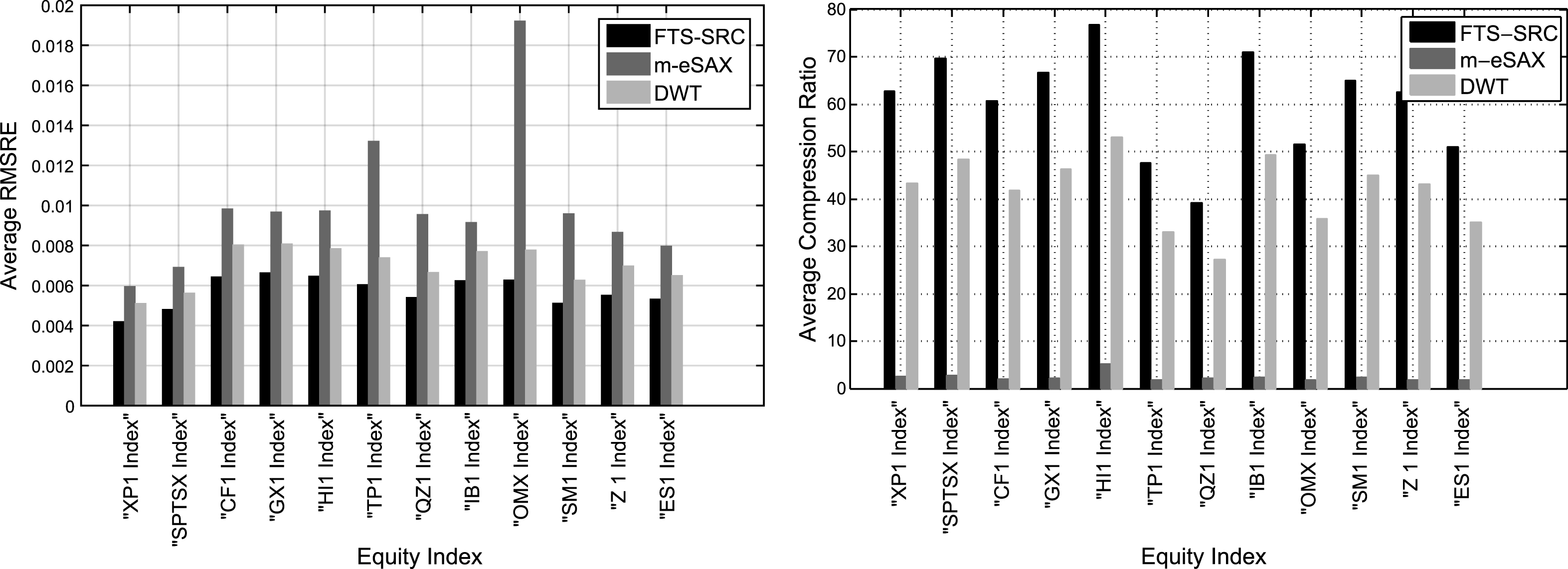
Fig.5

Original time series (Australian market) and its reconstruction using FTS-SRC, m-eSAX, and DWT (zoomed part (gray rectangle) is shown in the right plot along with some spikes (squares) introduced artificially by m-eSAX).

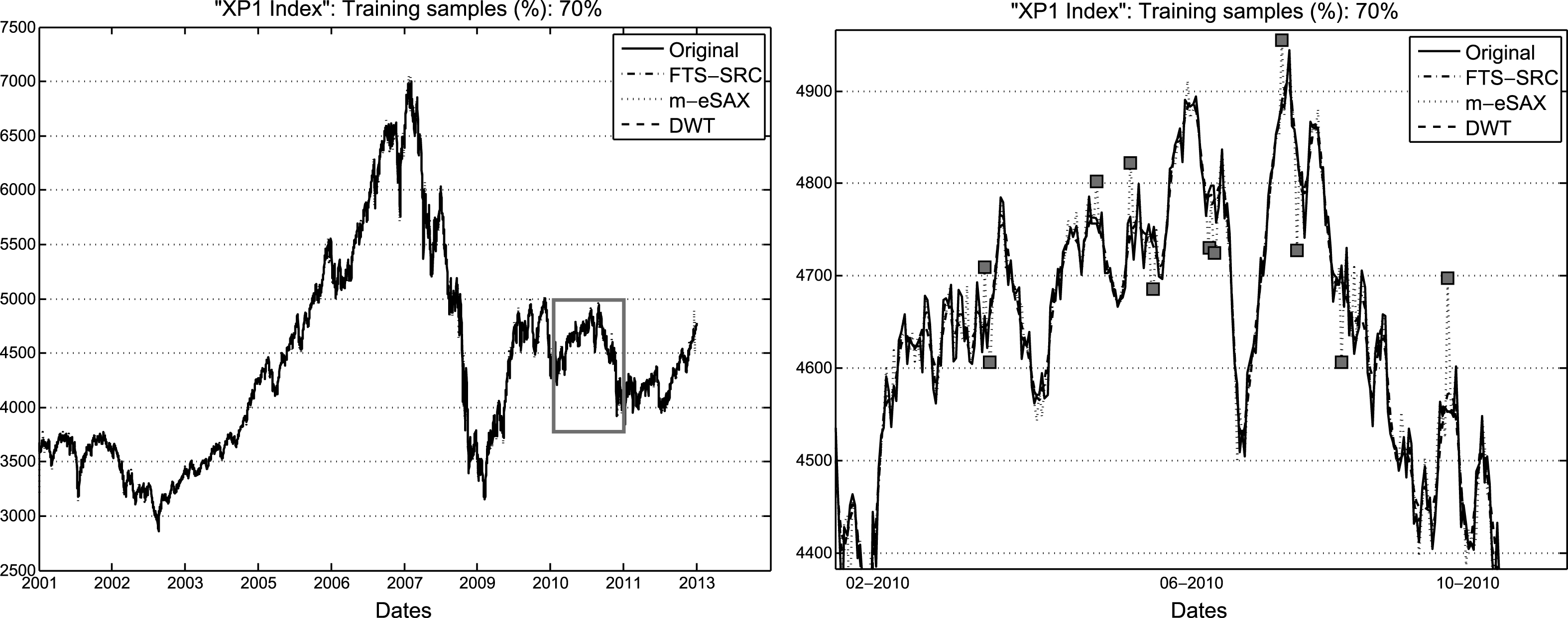
Fig.6

RMSRE (%) versus annualized volatility of logarithmic returns for the 12 equity markets, for the FTS-SRC, m-eSAX, and DWT representations (70% training samples).

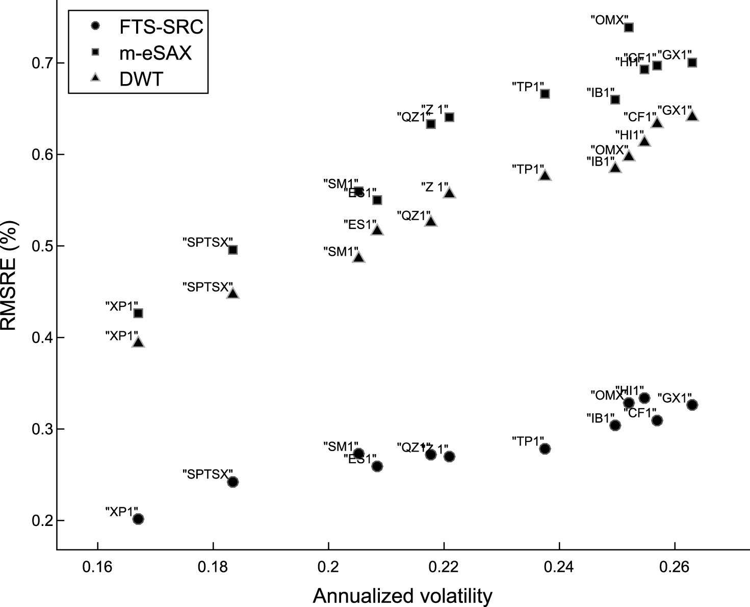
Fig.7

RMSRE (%) versus skewness of logarithmic returns for the 12 equity markets, for the FTS-SRC, m-eSAX, and DWT representations (70% training samples).

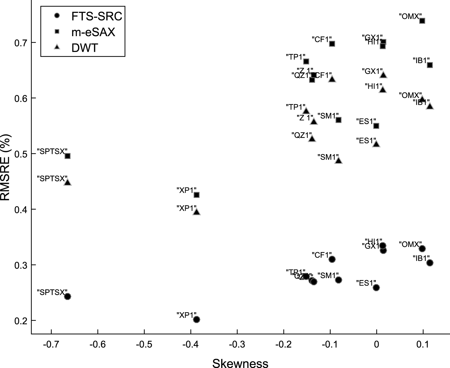
Fig.8

Moving annualized volatility (%) for XP1 index, estimated in monthly rolling windows with a weekly step-size. The ground truth volatility (MAVol) is compared against the volatility values estimated directly from the sparse patterns associated with FTS-SRC, m-eSAX, and DWT representations (70% training samples).

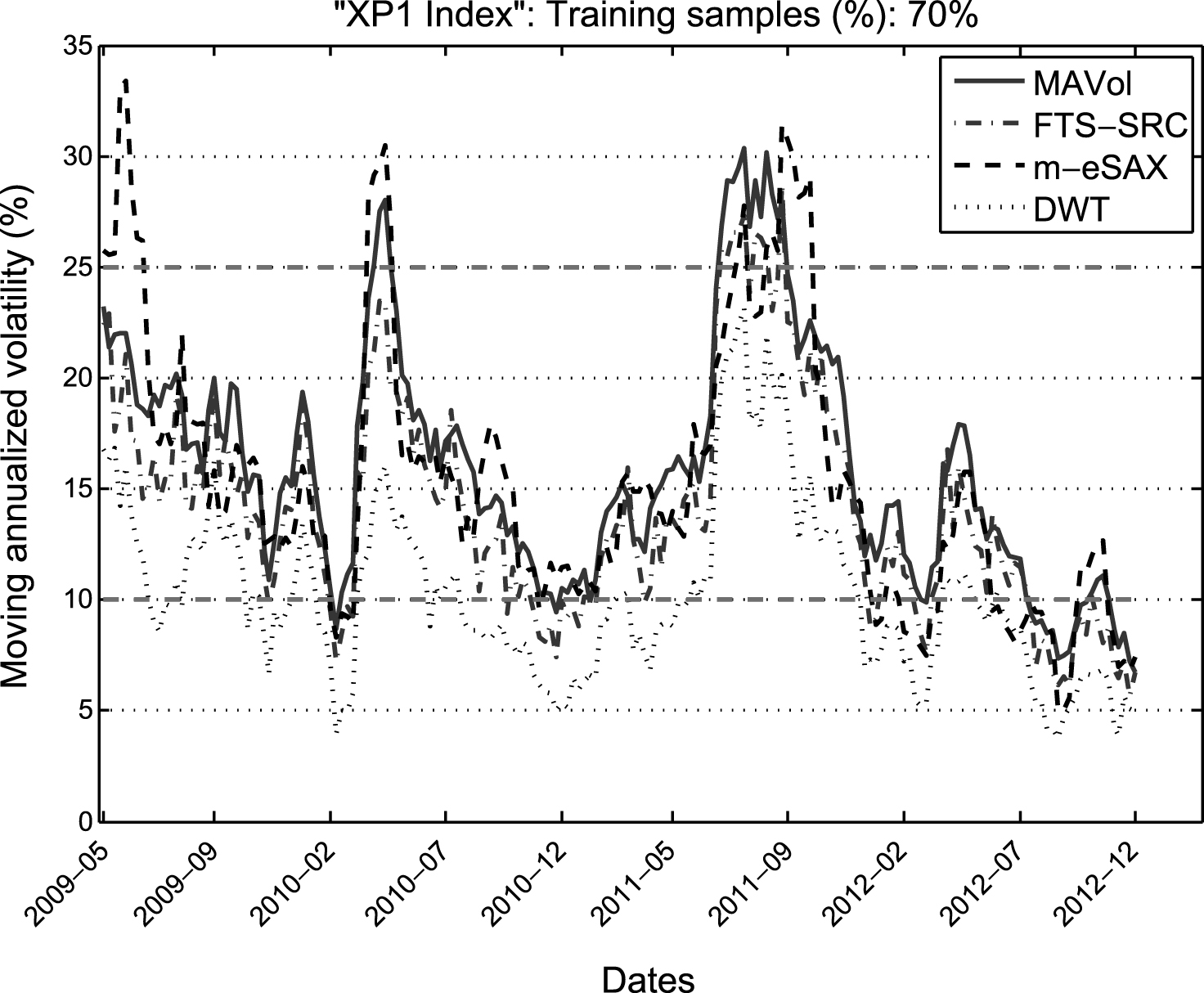
Fig.9

Success rates (%) of correctly identifying low, normal, and high annualized volatility windows based on the sparse patterns extracted via FTS-SRC, m-eSAX, and DWT for the 12 equity indexes. The overlaid curves correspond to the true number of low, normal, and high volatility windows, respectively.

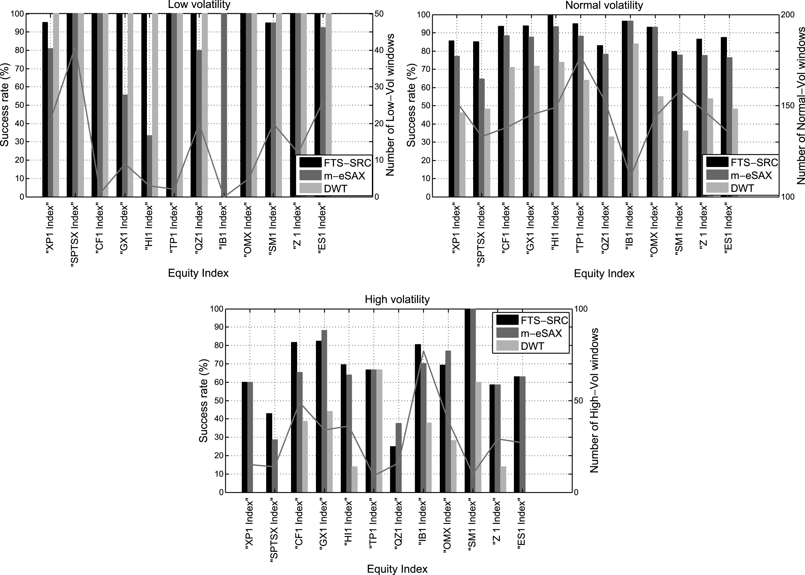
Table 1

Examples of dyadic alphabets for varying number of quantization bits Q

Quantization	Dyadic
bits (Q)	alphabet (A)
1	A={0,1}
2	A={00,01,10,11}
3	A={000,001,010,011,100,101,110,111}

Table 2

Statistics (average, volatility, and skewness) of returns (first difference of logarithms) for the 12 equity markets

Index	Average (%)	Volatility (%)	Skewness
XP1	2.158	16.70	-0.274
SPTSX	2.873	18.35	-0.461
CF1	-2.652	25.69	0.087
GX1	-0.725	26.31	0.249
HI1	5.291	25.47	0.208
TP1	-1.604	23.75	0.199
QZ1	4.556	21.78	-0.002
IB1	1.363	24.96	0.294
OMX	0.602	25.20	0.231
SM1	0.035	20.52	0.087
Z1	0.003	22.09	0.106
ES1	0.324	20.83	0.255

Table 3

Average RMSRE versus the percentage of training samples over 12 equity indexes for FTS-SRC, m-eSAX, and DWT-based representations

Method	Training samples (%)	Average RMSRE
	50	0.0057
FTS-SRC	60	0.0056
	70	0.0055
	50	0.0099
m-eSAX	60	0.0098
	70	0.0098
	50	0.0070
DWT	60	0.0070
	70	0.0070

Table 4

Major advantages (Pros) and limitations (Cons) of the three representation methods, FTS-SRC, m-eSAX, and DWT

	FTS-SRC	m-eSAX	DWT
Pros	✓ Automatic adaptation to complicated localized patterns	✓ Data adaptive	✓ Capable of representing extreme points
	✓ High compression rates	✓ High compression rates	✓ High compression rates
	✓ Independent of data distribution (Gaussian, non-Gaussian)	✓ Independent of data distribution (Gaussian, non-Gaussian)	✓ Independent of data distribution (Gaussian, non-Gaussian)
	✓ Increased robustness to limited training data	✓ Simple and computationally efficient implementation	✓ Computationally efficient implementation
	✓ No need for data normalization (e.g., local currencies are supported)		✓ No need for data normalization (e.g., local currencies are supported)
	✓ Correlations between distinct time series are exploited
Cons	× Increased computational cost for training the dictionary	× Poor representation of complicated localized patterns	× Non data-adaptive
		× Large amount of training (historical) data is necessary	× Large amount of training (historical) data is necessary
		× Estimated breakpoints are highly sensitive to available data	× Prior knowledge of data characteristics is required to choose optimally the wavelet decomposition
		× Data normalization is required (e.g., local currencies are not supported)	× Correlations between distinct time series are not exploited
		× Artificial spikes can be introduced during reconstruction
		× Correlations between distinct time series are not exploited